

Abstract
This paper presents methods to analyze functional brain networks and signals from graph spectral perspectives. The notion of frequency and filters traditionally defined for signals supported on regular domains such as discrete time and image grids has been recently generalized to irregular graph domains, and defines brain graph frequencies associated with different levels of spatial smoothness across the brain regions. Brain network frequency also enables the decomposition of brain signals into pieces corresponding to smooth or rapid variations. We relate graph frequency with principal component analysis when the networks of interest denote functional connectivity. The methods are utilized to analyze brain networks and signals as subjects master a simple motor skill. We observe that brain signals corresponding to different graph frequencies exhibit different levels of adaptability throughout learning. Further, we notice a strong association between graph spectral properties of brain networks and the level of exposure to tasks performed, and recognize the most contributing and important frequency signatures at different levels of task familiarity.
Index Terms: Functional brain network, network theory, graph signal processing, fMRI, motor learning, filtering
I. Introduction
The study of brain activity patterns has proven valuable in identifying neurological disease and individual behavioral traits [1]–[3]. The use of functional brain networks describing the tendency of different regions to act in unison has proven complementary in the analysis of similar matters [4]–[7]. It is not surprising that signals and networks prove useful in similar problems since the two are closely related. In this paper we advocate an intermediate path in which we interpret brain activity as a signal supported on the graph of brain connectivity. We show how the use of graph signal processing tools can be used to glean information from brain signals using the network as an aid to identify patterns of interest. The benefits of incorporating network information into signal analysis has been demonstrated in multiple domains. Notable examples of applications include video compression [8], breast cancer diagnostics [9], movie recommendation [10], and semi-supervised learning [11].
The fundamental GSP concepts that we utilize to exploit brain connectivity in the analysis of brain signals are the graph Fourier transform (GFT) and the corresponding notions of graph frequency components and graph filters. These concepts are generalizations of the Fourier transform, frequency components, and filters that are used in regular domains such as time and spatial grids [12]–[14]. As such, they permit the decomposition of a graph signal into components that represent different modes of variability. We can define low graph frequency components representing signals that change slowly with respect to brain connectivity networks in a well defined sense and high graph frequency components representing signals that change fast in the same sense. This is important because low and high temporal variability have proven important in the analysis of neurological disease and behavior [15], [16]. GFT based decompositions permit a similar analysis of variability across regions of the brain for a fixed time – a sort of spatial variability measured with respect to the connectivity pattern. We demonstrate here that it is useful in a similar sense; see e.g. Figs. 6, 7, 8, and 10.
Fig. 6.

Distribution of decomposed signals for the 6 week experiment. (a) Absolute magnitudes for all brain regions with respect to xL – brain signals varing smoothly across the network – averaged across all sample points for each individual and across all participants at the first scan session of the 6 week dataset. (b) With respect to xM and (c) with respect to xH – signals rapidly fluctuating across the brain. (d), (e), and (f) are averaged xL, xM and xH at the last scan session of the 6 week dataset, respectively. Only regions with absolute magnitudes higher than a fixed threshold are colored.
Fig. 7.
Distribution of decomposed signals for the 3 day experiment. (a), (b), and (c) are the absolute magnitudes for all brain regions with respect to xL, xM and xH, averaged across all sample points for each subject and across participants in the 3 day experiment, respectively. Regions with absolute value less than a threshold are not colored.
Fig. 8.
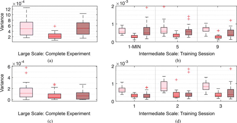
Temporal adaptations of spatial variations. Boxplots showing differences in temporal adaptabilities between brain activities with smooth (pink), moderate (red) and rapid (maroon) spatial variations, measured over the complete experiment for 6 week (a) and 3 day (c), and individual training sessions for 6 week (b) and 3 day (d) experiments. We measured the temporal adaptations using the variance of the averaged activities over the complete experiment or with individual training sessions. Compared to activities with moderate spatial variations, smooth (95% sessions pass t-test with p < 0.01) and rapid (65% sessions pass t-test with p < 0.005) spatial variations have significantly higher temporal adaptations.
Fig. 10.
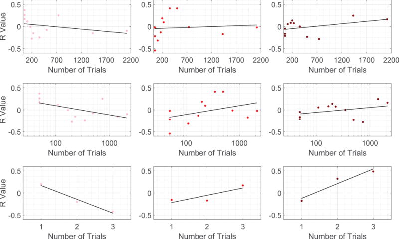
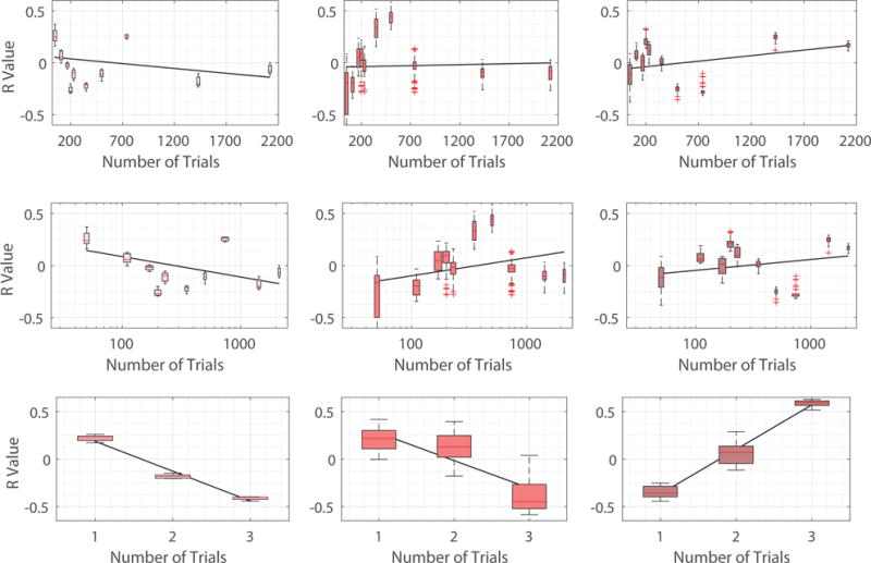
Scatter plots in which each point is for a specific training session (level of task familiarity), depicting the R value defined here as correlations between learning rate parameters and the norm of the decomposed signal of interest (Pink points in the Left: xL, Red points in the Middle: xM, and Maroon points in the Right: xH). Top row: 6 week experiment with number of trials described in linear scale. Middle row: 6 week experiment withe number of trials evaluated in logarithm scale. We examine 6 week experiment by ordering the number of trials in both linear and logarithm scales to alleviate the fact that number of trials are densely distributed towards small values. Bottom row: 3 day experiment in which the number of trials is represented by the 3 scanning sessions in the experiment.
The GSP studies in this paper are related to principal component analysis (PCA), which has been used with success in the analysis of brain signals [17], [18]. The difference with the GSP analysis we present here is that PCA implicitly assumes the brain network to be a correlation matrix and the signals to be drawn from a stochastic model. More importantly, whereas the GFT can be used to, e.g., decompose the signal into low, medium, and high frequency components, PCA is mostly utilized for dimensionality reduction; which in the language of this paper is tantamount to analyzing a few low graph frequency components. Another important difference is that PCA focuses on identifying variability across different realizations of brain signals, but the GFT identifies spatial variability of a single realization. GSP is also related to the spectral analysis of networks in general and Laplacians in particular [19], [20]. The difference in this case is that these spectral analyses yield properties of the networks. In GSP analyses, the network provides an underlying structure, but the interest is on signals expressed on this stratum.
Recent studies have already demonstrated that exploiting information from the underlying graph networks of structural brain connectivity to filter functional signals such as fMRI [21] and EEG [22] result in increased localization accuracy. The notion of investigating specific graph frequencies has just recently been introduced to capture key features of structural resting state networks (RSNs). Individual low frequencies have been identified to represent with low reconstruction error resting state networks related to visual and motor regions, and higher frequencies have been seen to well reconstruct more complex RSNs [23]. The research we present here extends these concepts by using GSP not only for investigating the underlying network as a whole, or individual frequencies on the underlying network, but to study how different ranges of frequencies capture significant information about the signal activation patterns, and applying this to dynamic, task-associated signals. These previous findings give high motivation for such an investigation.
The goal of this paper is to introduce GSP notions that can be used to analyze brain signals and to demonstrate their value in identifying patterns that appear when monitoring activity as subjects learn to perform a visual-motor task. Specifically, the contributions of this paper are: (i) To explain tools from the emerging field of GSP and show how they can be applied in analyzing brain signals. (ii) To evaluate the graph spectrum of brain functional network and to define artificial network construction methods that replicate the features of the graph spectrum of functional networks. (iii) To examine the temporal variation of brain signals corresponding to different graph frequencies when participants perform visual-motor learning tasks. (iv) To investigate the contribution of brain signals associated with different graph frequencies to the learning success at different stages of visual-motor learning.
We begin the paper with the introduction of basic notions of graphs and graph signals. Particular emphasis goes into the definition of the graph Fourier transform and the interpretation of graph frequency components as different modes of spatial variability measured with respect to the brain network (Section II-A). We also introduce the notion of graph filters and discuss the interpretation of graph low-pass, band-pass and high-pass filters as a local averaging operation (Section II-B). We point out that the discussion here is more extensive than necessary for readers familiar with GSP so that the paper is accessible to readers that are not necessarily familiar with the subject.
We then move on to describe two different experiments involving the learning of different visual-motor tasks by different sets of participants (Section III). We visualize the decomposed graph frequencies relating to the functional brain network (Section IV). We find that high graph frequencies of functional networks concentrate on visual and sensorimotor modules of the brain – the two brain areas well-known to be associated with motor learning [24], [25]. This motivates us to consider graph frequencies other than low frequency components, whereas the PCA-oriented approach has been focusing on low frequencies. We also describe the construction of a simple model to establish artificial networks with a few network descriptive parameters (Section IV-A). We observe that the model is able to mimic the properties of actual functional brain networks and we use them to analyze spectral properties of the brain networks (Section IV-B). The paper then utilizes graph frequency decomposition to visualize and investigate brain activities with different levels of spatial variation (Section V). It is noticed that the decomposed signals associated to different graph frequencies exhibit different levels of temporal variation throughout learning (Section V-A). Finally, we also define learning capabilities of subjects, and examine the importance of brain frequencies at different task familiarity by evaluating their respective correlation with learning performance at different task familiarities (Section VI). We find as learning progresses, we favor different levels of graph frequency components.
II. Graph Signal Processing
The interest of this paper is to study brain signals in which we are given a collection of measurements xi associated with each cortical region out of n different brain regions. An example signal of this type is an fMRI reading in which xi estimates the level of activity of brain region i. The collection of n measurements is henceforth grouped in the vector signal . A fundamental feature of the signal x is the existence of an underlying pattern of structural or functional connectivity that couples the values of the signal x at different brain regions. Irrespective of whether connectivity is functional or structural, our goal here is to describe tools that utilize this underlying brain network to analyze patterns in the neurophysiological signal x.
We do so by modeling connectivity between brain regions with a network that is connected, weighted, and symmetric. Formally, we define a network as the pair , where is a set of n vertices or nodes representing individual brain regions and represents weights of edges in the network with being the weight of the edge (i, j), in which . Since the network is undirected and symmetric we have that wij = wji for all (i, j). The weights wij = wji represent the strength of the connection between regions i and j, or, equivalently, the proximity or similarity between nodes i and j. In terms of the signal x, this means that when the weight wij is large, the signal values xi and xj tend to be related. Conversely, when the weight wij is small, the signal values xi and xj are not directly related except for what is implied by their separate connections to other nodes.
We adopt the conventional definitions of the degree and Laplacian matrices [26, Chapter 1]. The degree matrix is a diagonal matrix with its ith diagonal element . The Laplacian matrix is defined as the difference . The components of the Laplacian matrix are explicitly given by Lij = −wij and . Observe that the Laplacian is real, symmetric, diagonal dominant, and with strictly positive diagonal elements. As such, the matrix L is positive semidefinite. The eigenvector decomposition of L is utilized in the following section to define the graph Fourier transform and the associated notion of graph frequencies.
We note that brain networks, irrespective of whether their connectivity is functional [27] or structural [28], tend to be stable for a window of time, entailing associations between brain regions during captured time of interest. Brain activities can vary more frequently, forming multiple samples of brain signals supported on a common underlying network.
A. Graph Fourier Transform and Graph Frequencies
Given that the graph Laplacian L is real symmetric, it can be decomposed into its eigenvalue components,
| (1) |
such that for the set of eigenvalues , the diagonal eigenvalue matrix is defined as , and
| (2) |
is the eigenvector matrix. VH represents the Hermitian (conjugate transpose) of the matrix V. We assume the set of eigenvalues of the Laplacian L are ordered so that . The validity of (1) follows because the eigenvectors of symmetric matrices are orthogonal so that the definition in (2) implies that VHV = I. The eigenvector matrix V is used to define the Graph Fourier Transform of the graph signal x as we formally state next; see, e.g., [14].
Definition 1
Given a signal and a graph Laplacian accepting the decomposition in (1), the Graph Fourier Transform (GFT) of x with respect to L is the signal
| (3) |
The inverse (i)GFT of with respect to L is defined as
| (4) |
We say that x and form a GFT pair.
Observe that since VVH = I, the iGFT is, indeed, the inverse of the GFT. Given a signal x we can compute the GFT as per (3). Given the transform we can recover the original signal x through the iGFT transform in (4).
There are several reasons that justify the association of the GFT with the Fourier transform. Mathematically, it is just a matter of definition that if the vectors vk in (1) are of the form , the GFT and iGFT in Definition 1 reduce to the conventional time domain Fourier and inverse Fourier transforms. More deeply, if the graph is a cycle, the vectors vk in (1) are of the form . Since cycle graphs are representations of discrete periodic signals, it follows that the GFT of a time signal is equivalent to the conventional discrete Fourier transform; see, e.g., [29].
An important property of the GFT is that it encodes a notion of variability akin to the notion of variability that the Fourier transform encodes for temporal signals. To see this, define and expand the matrix product in (4) to express the original signal x as
| (5) |
It follows from (5) that the iGFT allows us to write the signal x as a sum of orthogonal components vk in which the contribution of vk to the signal x is the GFT component . In conventional Fourier analysis, the eigenvectors carry a specific notion of variability encoded in the notion of frequency. When k is close to zero, the corresponding complex exponential eigenvectors are smooth. When k is close to n, the eigenfunctions fluctuate more rapidly in the discrete temporal domain. In the graph setting, the graph Laplacian eigenvectors provide a similar notion of frequency. Indeed, define the total variability of the graph signal x with respect to the Laplacian L as
| (6) |
where in the second equality we expanded the quadratic form. It follows that the total variation TV(x) is a measure of how much the signal changes with respect to the network. For the edge (i, j), when wij is large we expect the values xi and xj to be similar because a large weight wij is encoding functional similarity between brain regions i and j. The contribution of their difference (xi − xj)2 to the total variation is amplified by the weight wij. If the weight wij is small, activities at brain regions i and j tend to be uncorrelated, and therefore the difference between the signal values xi and xj makes little contribution to the total variation. We can then think of a signal with small total variation as one that changes slowly over the graph and of signals with large total variation as those that change rapidly over the graph.
Consider the total variation of the eigenvectors vk and use the facts that Lvk = λkvk and to conclude that
| (7) |
It follows from (7) and the fact that the eigenvalues are ordered as , that the total variations of the eigenvectors vk follow the same order. Combining this observation with the discussion following (6), we conclude that when k is close to 0, the eigenvectors vk vary slowly over the graph, whereas for k close to n the eigenvalues vary more rapidly. Therefore, from (5) we see that the GFT and iGFT allow us to decompose the brain signal x into components that characterize different levels of variability. The GFT coefficients for small values of k indicate how much these slowly varying signals contribute to the observed brain signal x. On the other hand, the GFT coefficients for large values of k describe how much rapidly varying signals contribute to the observed brain signal x.
B. Graph Filtering and Frequency Decompositions
Given a graph signal x with GFT we can isolate the frequency components corresponding to the lowest KL graph frequencies by defining the filtered spectrum satisfying for k < KL and otherwise. The filter can be written as the diagonal matrix where the vector takes value 1 for frequencies smaller than KL and is otherwise null,
| (8) |
Utilizing the definitions of the GFT in (3) and the iGFT in (4), the spectral operation is equivalent to performing the following operations in the graph vertex domain
| (9) |
From the equality in (9), we can see that the signal xL contains the low graph frequency components of x, and so we say the matrix HL is a graph low-pass filter.
The filter admits an alternative representation as the expansion in terms of Laplacian powers [29]. The coefficients hLk in this expansion are elements of the vector where Ψ is the Vandermonde matrix defined by the eigenvalues of L, i.e.,
| (10) |
Since the eigenvalues are ordered in (10), the coefficients hLk tend to be concentrated in small indexes k, and the expansion is therefore dominated by small powers Lk. From this fact it follows that we can think of the graph low-pass filtered signal xL as resulting from a localized averaging of the elements of x. To understand this interpretation, simply note that L0x = x coincides with the original signal, Lx is an average of neighboring elements, L2x is an average of elements in nodes that interact via intermediate common neighbors, and, in general, Lkx describes interactions between k-hop neighbors. The fact that xL can be considered as a signal that follows from local averaging of x implies that xL has smaller total variation than x and is consistent with the interpretation of low graph frequencies presented in Section II-A. We point out that the definition assumes the inverse matrix Ψ−1 exists. This holds true if the graph Laplacian does not have duplicate eigenvalues, which is the case for all functional brain networks examined in the paper.
Other types of graph filters can be defined analogously to study interactions between signal components other than the local interactions captured in xL. Apart from the graph low-pass filter HL, we also consider a graph band-pass filter HM and a graph high-pass filter HH, whose graph frequency responses are defined as
| (11) |
| (12) |
The definitions in (8), (11), and (12) are such that the low-pass filter takes the lowest KL graph frequencies, the band-pass filter captures the middle KM graph frequencies, and the high-pass filter the highest n − KL − KM frequencies. The three filters are defined such that the graph frequencies of their respective interest are mutually exclusive yet collectively exhaustive. As a result, if we use xM:= HMx and xH:= HHx to respectively denote the signals filtered by the band-pass and high-pass filters, we have that the original signal can be written as the sum x = xL + xM + xH. This gives a decomposition of x into low, medium, and high frequency components which respectively represent signals that have slow, medium, and high variability with respect to the connectivity network between brain regions. This decomposition is utilized in this paper to analyze brain activity patterns associated with the learning of visual-motor tasks.
III. Brain Signals during Learning
We considered two experiments in which subjects learned a simple motor task [30]–[32]. In the experiments, fourty-seven right-handed participants (29 female, 18 male; mean age 24.13 years) volunteered with informed consent in accordance with the University of California, Santa Barbara Internal Review Board. After exclusions for task accuracy, incomplete scans, and abnormal MRI, 38 participants were retained for subsequent analysis.
Twenty individuals participated in the first experimental framework. The experiment lasted 6 weeks, in which there were 4 scanning sessions, roughly at the start of the experiment, at the end of the 2nd week, at the end of the 4th week, and at the end of the experiment, respectively. During each scanning session, individuals performed a discrete sequence-production task in which they responded to sequentially presented stimuli with their dominant hand on a custom response box. Sequences were presented using a horizontal array of 5 square stimuli with the responses mapped from left to right such that the thumb corresponded to the leftmost stimulus. The next square in the sequence was highlighted immediately following each correct key press; the sequence was paused awaiting the depression of the appropriate key if an incorrect key was pressed. Each participant completed 6 different 10-element sequences. Each sequence consists of two squares per key. Participants performed the same sequences at home between each two adjacent scanning sessions, however, with different levels of exposure for different sequence types. Therefore, the number of trials completed by the participants after the end of each scanning session depends on the sequence type. There are 3 different sequence types (MIN, MOD, EXT) with 2 sequences per type. The number of trials of each sequence type completed after each scanning session averaged over the 20 participants is summarized in Fig. 1. During scanning sessions, each scan epoch involved 60 trials, 20 trials for each sequence type. Each scanning session contained a total of 300 trials (5 scan epochs) and a variable number of brain scans depending on how quickly the task was performed by the specific individual.
Fig. 1.
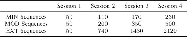
Relationship between training duration, intensity, and depth for the first experimental framework. The values in the table denote the number of trials (i.e., “depth”) of each sequence type (i.e., “intensity”) completed after each scanning session (i.e., “duration”) averaged over the 20 participants.
Eighteen subjects participated in the second experimental framework. The experiment had 3 scanning sessions spanning the three days. Each scanning session lasted roughly 2 hours and no training was performed at home between adjacent scanning sessions. Subjects responded to a visually cued sequence by generating responses using the four fingers of their nondominant hand on a custom response box. Visual cues were presented as a series of musical notes on a pseudomusical staff with four lines such that the top line of the staff mapped to the leftmost key pressed with the pinkie finger. Each 12-note sequence randomly ordered contained three notes per line. Each training epoch involved 40 trials and lasted a total of 245 repetition times (TRs), with a TR of 2,000 ms. Each training session contained 6 scan epochs (240 trials) and lasted a total of 2,070 scan TRs.
In both experiments participants were instructed to respond promptly and accurately. Repetitions (e.g., “11”) and regularities such as trills (e.g., “121”) and runs (e.g., “123”) were excluded in all sequences. The order and number of sequence trials were identical for all participants. Participants completed the tasks inside the MRI scanner for scanning sessions.
Reordering with fMRI was conducted using a 3.0 T Siemens Trio with a 12-channel phased-array head coil. For each functional run, a single-shot echo planar imaging sequence that is sensitive to blood oxygen level dependent (BOLD) contrast was utilized to obtain 37 (the first experiment) or 33 (the second experiment) slices (3mm thickness) per repetition time (TR), an echo time of 30 ms, a flip angle of 90°, a field of view of 192 mm, and a 64 × 64 acquisition matrix. Image preprocessing was performed using the Oxford Center for Functional Magnetic Resonance Imaging of the Brain (FMRIB) Software Library (FSL), and motion correction was performed using FMRIB’s linear image registration tool. The whole brain is parcellated into a set of n = 112 regions of interest that correspond to the 112 cortical and subcortical structures anatomically identified in FSL’s Harvard-Oxford atlas. The choice of parcellation scheme is the topic of several studies in resting-state [33], and task-based [34] network architecture. The question of the most appropriate delineation of the brain into nodes of a network is open and is guided by the particular question one wants to ask. We use Harvard-Oxford atlas here because it is consistent with previous studies of task-based functional connectivity during learning [30], [31]. The threshold in probability cutoff settings of Harvard Oxford atlas parcellation is 0 so that no voxels were excluded.
For each individual fMRI dataset, we estimate regional mean BOLD time series by averaging voxel time series in each of the n regions. We evaluate the magnitude squared spectral coherence [35] between the activity of all possible pairs of regions to construct n × n functional connectivity matrices W. Besides, for each pair of brain regions i and j, we use t-statistical testing to evaluate the probability pi,j of observing the measurements by random chance, when the actual data are uncorrelated [36]. In the 3 day dataset, the value of all elements with no statistical significance (pi,j > 0.05) [37] are set to zero; the values remain unchanged otherwise. In the 3 day experiment, a single brain network is constructed for each participant. Thresholding is applied because the networks are for the entire span of the experiment and many entries in W would be close to zero without threshold correction. In the 6 week experiment, due to the long duration of the experiment, we build a different brain network per scanning session, per sequence type for each subject. Because each network describes the functional connectivity for one training session given a subject, not many entries will be removed even in the presence of threshold correction; consequently, no thresholding is applied for the 6 week dataset. We normalize the regional mean BOLD observations at any sample time t and consider such that the total energy of activities at all structures is consistent at different t to avoid extreme spikes due to head motion or drift artifacts in fMRI.
IV. Brain Network Frequencies
In this section, we analyze the graph spectrum brain networks of the dataset considered. For the brain network W of each subject, we construct its Laplacian L = D − W, and evaluate the total variation TV(vk) [cf. (7)] for each eigenvector vk. Fig. 2 (a) and (c) plot the total variation of all graph eigenvectors averaged across participants of the 6 week training experiment and 3 day experiment, respectively. In both experiments, the Laplacian eigenvectors associated with larger indexes fluctuate more on the network. Another observation is that with respect to graph frequency indices 0 < k < 100, the total variation increases almost linearly.
Fig. 2.
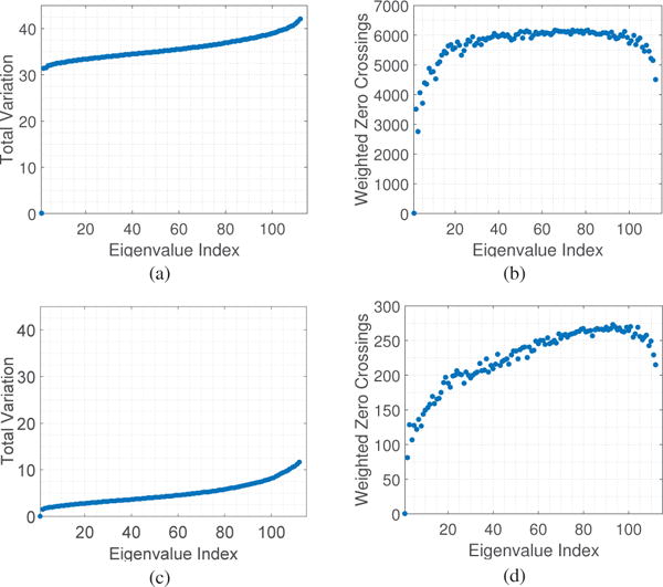
(a) Total variation TV(vk) and (b) weighted zero crossings ZC(vk) of the graph Laplacian eigenvectors for the brain networks averaged across participants in the 6 week training experiment. (c) and (d) present the values for the 3 day experiment. In both cases, the Laplacian eigenvectors associated with larger indexes vary more on the network and cross zero relatively more often, confirming the interpretation of the Laplacian eigenvalues as notions of frequencies. Besides, note that total variation increases relatively linearly with indexes.
Besides total variation, the number of zero crossings is used as a measure of the smoothness of signals with respect to an underlying network [14]. Since brain networks are weighted, we adapt a slightly modified version – weighted zero crossings – to investigate the given graph eigenvector vk
| (13) |
In words, weighted zero crossings evaluate the weighted sum of the set of edges connecting a vertex with a positive signal to a vertex with a negative signal. Fig. 2 (b) and (d) demonstrate the weighted zero crossings of all graph eigenvectors averaged across subjects of the 6 week and 3 day experiments, respectively. The weighted zero crossings increase almost proportionally with graph frequency index k until they eventually level off for 0 ≤ k ≤ 100. For k greater than 100, though, eigenvectors associated with higher graph frequencies exhibit lower weighted zero crossings.
It would be interesting to examine where the associated eigenvectors lie anatomically, and the relative strength of their values. To facilitate the presentation, we consider three sets of eigenvectors, , and , and compute the absolute magnitude at each of the n cortical and subcortical regions averaged across participants and across all graph frequencies belonging to each of the three sets. Fig. 3 presents the average magnitudes for the two experimental frameworks considered in the paper using BrainNet [38], where brain regions with absolute magnitudes lower than a fixed threshold are not colored. Throughout the paper, the parameter KL is set as 40 and KM is set as 32. This combination yields three roughly equally-sized components with one piece corresponding to the 40 lowest graph frequencies and another piece corresponding to the 40 highest frequencies. The results presented in the paper are robust with the choice of parameters: we examined the results for KL and KM in the range of 32 to 42, inclusive, and found similar observations as the ones presented. To demonstrate that, Fig. 4 presents the range of correlation coefficients calculated between the frequency ranges selected for this paper and all frequency ranges for KL and KM between 32 and 42, inclusive, giving 120 correlation values for each box plot. The correlation coefficients reported are a quantification of similarity measure when we examine the similarity between two vectors, given as the absolute magnitudes passing the given threshold across all brain regions. An investigation of cosine similarity gives high similarities as well. We have also conducted robustness testing in our analysis of learning rate (Section VI) and have plotted our results obtained from using all 121 possible frequency ranges (Fig. 12) and have quantified the robustness of parameters in Fig. 11.
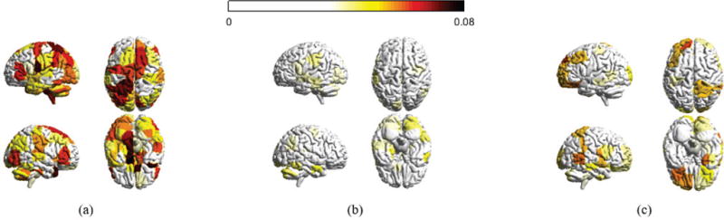
Fig. 3.
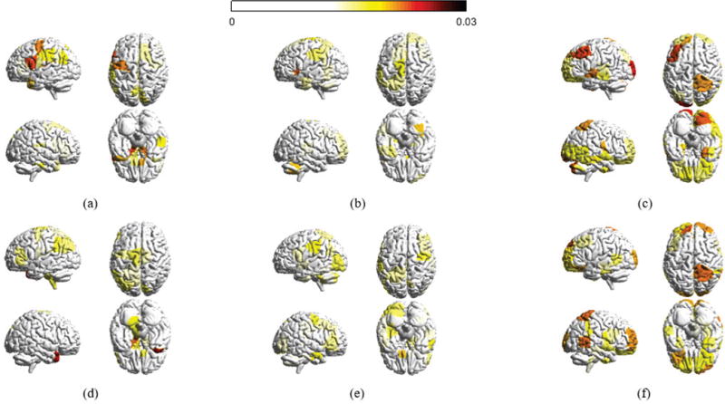
Absolute magnitude at each of the n cortical structures averaged across participants in the 6 week experiment and averaged across all frequency components in (a) the set of low graph frequencies , (b) the set of middle graph frequencies , and (c) the set of high graph frequencies (d)–(f) presents the average absolute magnitudes for the 3 day experiment. Only brain regions with absolute magnitudes higher than a fixed threshold (0.015) are colored. The magnitudes at different brain regions across the datasets are significantly similar in the low and high graph frequencies (correlation coefficients 0.5818 and 0.6616, respectively). The brain regions with high magnitude values significantly overlap with the visual and sensorimotor modules, in which more than 60% of values greater than the threshold belong to the visual and sensorimotor modules.
Fig. 4.
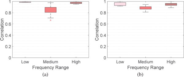
Box plots demonstrating the robustness of parameters chosen for different frequency ranges for the absolute magnitudes across brain regions for (a) 6 week and (b) 3 day experiments. Each box plot presents the correlation coefficients between the frequency range selected for this paper and all frequency ranges for KL and KM between 32 and 42, inclusive.
Fig. 12.
Robustness testing to show similar trends as observed in Fig. 10. Each box is for a specific training session (level of task familiarity), depicting the R values obtained from changing the frequency ranges of KL and KM between 32 and 42, inclusive. As such, the R value is defined here as correlations between learning rate parameters and the norm of the decomposed signal of interest for a specific frequency range. Each box contains R values for 121 different combinations of frequency ranges.
Fig. 11.
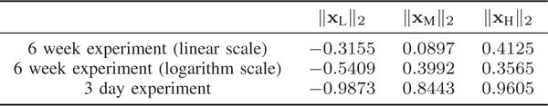
Pearson correlation coefficients for robustness testing, as comparable to Fig. 9. Each correlation coefficient is between the number of trials (level of task familiarity) and the average R value obtained at each trial. As such, each trial contains 121 R values for the different frequency ranges considered for KL and KM between 32 and 42, inclusive. Each R value is defined as the correlation between learning rate parameters and the norm of the decomposed signal of interest for a given frequency range.
A. Artificial Functional Brain Networks
An approach to analyze the complex networks is to define a model to generate artificial networks [39], [40]. The main motivation of an artificial network model is to use them to analyze complex brain networks. Examples of such models include the Barabási-Albert model for scale free networks [41] and recent developments and insights on weighted network models [40]. Here we present a framework to construct artificial networks that can be used to mimic the functional brain networks with only a few parameter inputs. The model is related to weighted block stochastic model [42], but involves more aspects like individual variance and analyzes links independent of their connectivity strength to other brain regions. The output of the method would be a symmetric network with edge weights between 0 and 1 without self-loops.
To begin, suppose the desired network has two clusters of nodes and The algorithm requires the average edge weight μ1 for connections between nodes of the first cluster , average edge weight μo for links between nodes of the other cluster , and average edge weight μ1o for inter-cluster connections. To reflect the fact that the edge weights on some links are independent of their joining vertices, for each edge within , with probability , its weight is randomly generated with respect to uniform distribution between 0 and 1, and with probability , its weight is randomly generated with respect to uniform distribution . The parameter determines the percentage of edges whose weights are selected irrespective of their actual locations To further simulate the observation that different participants may possess distinctive brain networks, if the edge weight is randomly generated from a uniform distribution , it is then perturbed by where controls the level of perturbation. The edge weights for connections within cluster are generated similarly: with probability , the edge weight is randomly chosen from the uniform distribution before being contaminated by . The edge weights for connections between clusters and are formed analogously μ1o. The method presented here can be easily generalized to analyze brain networks with more regions of interest, i.e. by specifying sets of regions of interest and by detailing the expected correlation values on each type of connection between different regions.
Remark 1
At one extreme we can make each node i belonging to a different set . Then the method requires the inputs of expected weights for all nodes, or alternatively speaking, the expected network. At the other extreme, there is only one set of nodes , and then the method is highly akin to a network with edge weights completely randomly generated. Any construction of interest would have some prior knowledge regarding the community structure. Therefore, the method proposed here can be used to see if the network constructed with the specific choice of community structure highly simulate the key properties of the actual network, and can be used to examine the evolution of community structure in the brain throughout the process to master a particular task.
B. Spectral Properties of Brain Networks
In this section, we analyze graph spectral properties of brain networks. Given the graph Laplacian, we examine the fluctuation of its eigenvectors on different types of connections in the brain network [25]. More specifically, given an eigenvector vk, its variation on the visual module is defined as
| (14) |
where denotes the set of nodes belonging to the visual module. The measure TVvisual(vk) computes the difference for signals on the visual module for each unit of edge weight. To facilitate interpretation, we only consider three sets of eigenvectors , and . We then compute the visual module total variation averaged over eigenvectors , and as well as similarly. Besides , we also examine the level of fluctuation of eigenvectors on edges within the motor module, denoted as TVmotor, and on connections belonging to brain modules other than the visual and motor module TVothers. Further, there are links between two separate brain modules, and to assess the variation of eigenvectors on those links, we define total variations between the visual and motor modules
| (15) |
where denotes the set of nodes belonging to the motor module. Total variations TVvisual-others between the visual and other modules, and total variations TVmotor-others between the motor and other modules are defined analogously. We chose to study visual and motor modules separately from other brain modules because of their well-known associations with motor learning [24], [25].
Fig. 5 (a) presents boxplots of the variation for eigenvectors of different graph frequencies measured over different types of connections across participants, at the start of the six week training. Despite that total variation of eigenvectors should increase with their frequencies, the variation on the other module of eigenvectors associated with low frequencies are higher than (pass t-test with p < 0.0001). This observation is discussed in detail in Section IV-C.
Fig. 5.
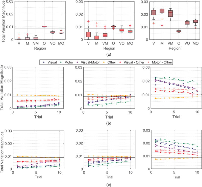
Spectral property of brain networks in the 6 week experiment. (a) Left: Averaged total variation of eigenvectors vk for 6 different types of connections of the brain averaged across all eigenvectors associated with low graph frequencies , across all participants and scan sessions. Middle: Across all eigenvectors associated with mid-range graph frequencies . Right: Across all eigenvectors with high graph frequencies . (b) Median total variations of brain networks across participants of different scanning sessions and different sequence types with respect to the level of exposure of participants to the sequence type at the scanning session. Relationship between training duration, intensity, and depth is summarized in Fig. 1. Value of 1 on the x-axis in the figures refers to minimum exposure to sequences (all 3 sequence types of the first session), and value of 10 on the x-axis denotes the maximum exposure to sequences (EXT sequence types of the fourth session). An association between spectral property of brain networks and the level of exposure is clearly observed (average correlation coefficient 0.8164). (c) Median total variations evaluated upon artificial networks. Spectral properties of actual brain networks can be closely simulated using a few parameters. The main text gives all correlation values for similarity between variance among subjects and between correlations of training intensity.
Next we study how the graph spectral properties of brain networks evolve as participants become more familiar with the tasks. Fig. 5 (b) illustrates the median of the variation for eigenvectors of different graph frequencies measured over different types of connections across subjects, at 10 different levels of exposure in the six week training. As participants become more acquainted with the assignment, their brain networks display lower variation in the visual and motor modules and higher variation in the other modules for low and middle graph frequencies, and the exact opposite is true for high graph frequencies. The association with training intensity is statistically significant (average correlation coefficient r = 0.8164).
C. Discussion
Firstly, we examine why we see a decrease in zero crossings of graph frequencies when k is greater than 100 in Fig. 2. A detailed analysis shows this is because the functional brain networks are highly connected with nearly homogeneous degree distribution, and consequently each high graph frequency tends to have a value with high magnitude at one vertex of high degree and similar values at other nodes, resulting in a smaller global zero crossings for eigenvectors associated with very high frequencies.
Secondly, in terms of the visualization of graph frequencies in Fig. 3, the most interesting finding relates to the eigenvectors associated with high graph frequencies. The magnitudes at different brain regions for high frequencies are significantly similar across the two datasets investigated (correlation coefficient 0.6616). There are very few noticeable brain regions in which the absolute magnitude highlighted in the first dataset is not likewise highlighted in the second. Given the different experiment setups, it would not be uncommon to observe large variations across datasets. However, the fact that we see the majority of brain regions similarly highlighted in the two experiments solidifies our understanding that eigenvector decomposition captures general signatures, as opposed to task-specific realizations. Additionally, brain regions with high magnitude values are highly alike (greater than 60% overlap) to the visual and sensorimotor cortices [43]. This is likely to be a consequence of the fact that visual and motor regions are more strongly connected with other structures, and hence an eigenvector with a high magnitude on visual or motor structures would result in high global spatial variation. The eigenvectors of low graph frequencies are more spread across the networks, resulting in low global variations. The middle graph frequencies are less interesting – the magnitudes at most regions (greater than 90%) do not pass the threshold, and little associations (correlation coefficient 0.3529) can be found between the eigenvectors of the 6 week and 3 day experiments.
Thirdly, to better interpret the meaning of variations for specific types of connections, we construct artificial networks as described in Section IV-A with visual and motor modules as regions of interest, and consider other modules to be brain regions other than visual and motor modules. We observe that there are three contributing factors that cause the variation within a specific module to become higher for higher eigenvectors and to become lower for lower eigenvectors: (i) Increases in the average edge weight for connections within the module, (ii) Increments in the average edge weight for links between this module to other module, and (iii) Escalation in the average edge weight for associations within the other module. This can also be observed by analyzing closely the definition of total variation. If a module is highly connected, in order for the eigenvector associated with a low graph frequency to be smooth on the entire network, it has to be smooth on the specific module, resulting in a low value in the variation of an eigenvector associated with a low graph frequency with respect to the module of interest. Similarly, the increase in the variation of connections between two modules, e.g. between visual and other modules are resulted from: (i) The growth in the average edge weight for connections between visual and other modules, or (ii) The augmentation of average weight for links within the other module. The graph spectral properties as in Fig. 5 (a) are observed because (i) visual and motor modules are themselves highly connected, and (ii) visual module is also strongly linked with motor module.
Finally, in analyzing the evolution of graph spectral properties as participants become more familiar with the tasks, following the interpretations based on artificial network analysis, this evolution in graph spectral properties of brain networks is mainly caused by the decrease in values of connections within visual and motor modules and between the visual and motor modules. An interesting observation is that the values in the variation of eigenvectors associated with high frequencies decline with respect to the visual module much faster than that of motor module, even though the visual module is more strongly connected throughout training compared to the motor module. A deep analysis using artificial networks shows that this results from the following three factors: (i) Though more strongly connected compared to the motor module, connections within the visual module weaken very quickly, (ii) The motor module is more closely connected with the other module than the link between the visual module to the other module, and (iii) Association levels within the other module stay relatively constant. Therefore, as participants become more exposed to the tasks, compared to the visual module, the motor module becomes more strongly connected. The graph spectral properties of actual brain networks and their evolution can be closely imitated using artificial networks as plotted in Fig. 5 (c). The artificial network created for our analysis best imitated the real brain networks with parameters pε of 0.10, uε of 0.10, and δ of 0.01. The average edge weights μ for visual (ν), motor (m), other (o), and inter-connecting regions are μν = 0.6028, μm = 0.4902, μo = 0.3098, μνm = 0.3985, μνo = 0.3181, and μmo = 0.3271. The correlation coefficients of association with training intensity between real and artificial networks for low, medium, and high graph frequencies are 0.6436, 0.7187 and 0.8457, respectively. Additionally, the variation among participants in real dataset can be closely mimicked using artificial network model we proposed, with correlation coefficients 0.9338, 0.9660, and 0.9486 for low, medium, and high graph frequencies, respectively. The analysis for the three day training dataset is highly similar (correlation coefficients 0.9834, 0.9186, and 0.9674 for low, medium, and high graph frequencies, respectively) and for this reason we do not present and analyze it separately here.
V. Frequency Decomposition of Brain Signals
The previous sections focus on the study of brain networks and their graph spectral properties. In this section, we investigate brain signals from a GSP perspective, and analyze the brain signals by examining the decomposed graph signals xL, xM, and xH with respect to the underlying brain networks. We compute the absolute magnitude of the decomposed signal xL for each brain region averaged across all sample signals for each individual during a scan session and then averaged across all participants. Similar aggregation is applied for xM and xH.
Fig. 6 presents the distribution of the decomposed signals corresponding to different levels of spatial variations for the first scan session (top row) and the last scan session (bottom row) in the 6 week experiment. Fig. 7 exhibits how the decomposed signals are distributed across brain regions in the 3 day experiment. Brain regions with absolute magnitudes lower than a fixed threshold are not colored.
A. Temporal Variation of Graph Frequency Components
We analyze temporal variation of decomposed signals with respect to different levels of spatial variations. To this end, we evaluate the variance of the decomposed signals over multiple temporal scales – over days and minutes – for the two experiments. We describe the method specifically for xL for simplicity and similar computations were conducted for xM and xH. At the macro timescale, we average the decomposed signals xL for all sample points within each scanning session with different sequence type, and evaluate the variance of the magnitudes of the signals [15] across all the scanning sessions and sequence types. For the 6 week experiment, there are 4 scanning sessions and 3 different sequence types, so the variance is with respect to 12 points. For the 3 day experiment, there are 3 scanning sessions and only 1 sequence type, so the variance is for 3 points. As for the micro or minute-scale, we average the decomposed signals xL for all sample points within each minute, and evaluate the variance of the magnitudes of the averaged signals across all minute windows for each scanning session with different sequence types. The evaluated variance is then averaged across all participants of the experiment of interest.
Fig. 8 displays the variance of the decomposed signals xL, xM and xH at two different temporal scales of the two experiments. For the 6 week dataset, 3 session-sequence combinations, with the number proportional to the level of exposure of participants to the sequence (1-MIN refers to MIN sequence at session 1, 5 denotes MIN sequence at session 4, 9 entails EXT sequence at session 3) are selected out of the 12 combinations in total for a cleaner illustration, but all the other session-sequence combinations exhibit similar properties.
B. Discussion
A deep analysis of Figs. 6 and 7 yields many interesting aspects of graph frequency decomposition. First, for xL, the magnitudes on adjacent brain regions tend to possess highly similar values, resulting in a more evenly spread brain signal distribution, where as for xH, neighboring signals can exhibit highly dissimilar values; this corroborates the motivation to use graph frequency decomposition to segment brain signals into pieces corresponding to different levels of spatial fluctuations. Second, decomposed signals for a specific level of variation, notedly xH, are highly similar with respect to different scan sessions in an experiment as well as with respect to the two experiments with different sets of participants. The correlation coefficient between datasets for high graph frequencies is 0.6469. Third, recall that we normalize the brain signals at every sample point for all subjects, and for this reason signals xL, xM and xH would be similarly distributed across the brain if nothing interesting happens at the decomposition. However, in both Figs. 6 and 7, it is observed that many brain regions possess magnitudes higher than a threshold in xL (∼ 60% pass) and xH (∼ 20% pass) while not many brain regions pass the thresholding with respect to xM (∼ 3% pass). It has long been understood that the brain combines some degree of disorganized behavior with some degree of regularity and that the complexity of a system is high when order and disorder coexist [44]. xL varies smoothly across the brain network and therefore can be regarded as regularity (order), whereas xH fluctuates rapidly and consequently can be considered as randomness (disorder). This evokes the intuition that graph frequency decomposition segments a brain signal x into pieces xL and xH, which reflect order and disorder (and are therefore more interesting), as well as the remaining xM.
For the variance analysis, it is expected for the low graph frequency components (smooth spatial variation) to exhibit the smallest temporal variations, exceeded by medium and then high counterparts. Nonetheless, it is observed that brain activities with smooth spatial variations exhibit the most rapid temporal variation. Because it has been shown that temporal variation of observed brain activities is associated with better performance in tasks [15], this indicates a stronger contribution of low graph frequency components during the learning process. Furthermore, since the measurements were normalized such that the total energy of overall brain activities stayed constant at different sampling points, the rapid temporal changes of low graph frequency components should be accompanied by fast temporal variation of some other components, which are found to be high frequency components in all cases. Because these results were consistent for all of the temporal scales and datasets that we examined, and the association between temporal variability and positive performance has been established [16], we concluded that brain activities with smooth or rapid spatial variations offer greater contributions during learning. The graph frequency signatures at different stages of learning is analyzed in the next section.
VI. Frequency Signatures of Task Familiarity
Given that the decomposed signals exhibit interesting perspectives, it is natural to probe whether the signals corresponding to different levels of spatial variations associate with learning. To this end, we first describe how learning rate is evaluated. Given a participant, for each sequence completed, we defined the movement time M as the difference between the time of the first button press and the time of the last button press during a single sequence. We then estimate the participant’s learning rate by fitting an exponential function (plus a constant) using the robust outlier correction [45] to the sequence of movement times M
| (16) |
where t is a sequence representing the time index, κ is the exponential drop-off parameter (which we call the “learning rate parameter”) used to describe the early and fast rate of improvement, and c1 and c2 are nonnegative constants. Their sum c1 + c2 is an estimation of the starting speed of the participant of interest prior to training, while the parameter c2 entails the fastest speed to complete the sequence attained by that participant after extended training. A negative value of κ indicates a decrease in movement time M(t), which is thought to indicate that learning is occurring [46]. We chose exponential because it is viewed as the most statistically robust choice [47]. Further, the approach that we used has the advantage of estimating the rate of learning independent of initial performance or performance ceiling.
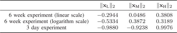
We evaluate the learning rate for all participants at each scanning session, and then compute the correlation between the norm ║xL║2 of the decomposed signal corresponding to low spatial variation and the learning rates across subjects. The correlation (R value) between the norms ║xM║2 as well as ║xH║2 and learning rates are also calculated. Fig. 10 plots the Pearson correlation coefficients at all scanning sessions of the two experiments considered. The horizontal axis denotes the level of exposure of participants to the sequence – which day in the 3 day experiment and how many number of trials participants have completed at the end of the scanning session in the 6 week experiment. Points are densely distributed for small number of trials in the 6 week experiment, so to mitigate this effect, we also plot the points by taking the logarithm of numbers of trials completed. We emphasize that due to normalization at each sampling point, the correlation values would all be 0 if graph frequency decomposition segments brain signals into three equivalent pieces. There are scan sessions where the correlation is of particular interest, however the most noteworthy observation is the change of correlation values with the level of exposure for participants.
In general, for xL corresponding to smooth spatial variation, we see a gradually decreasing trend in correlation with learning as training progresses. Although not all training sessions can be fit to this pattern (i.e. trials 500 and 740), it is still visible that the correlation with learning is above zero (≈ 0.25) at the start of the training when participants perform the task for the first time and gradually shifts to below zero (≈ −0.25) at the end of the experiment when individuals are highly familiar with the sequence. For xH corresponding to vibrant spatial variation, its correlation with learning is below zero (≈ −0.2) at the start of the training, and gradually increases throughout training until it is above zero (≈ 0.25) at the end of the experiment, with the exception of trials 500 and 740. This is the exact opposite of xL. For xM, correlation between its norm ║xM║2 with learning rate generally increases with the intensity of training. However, this trend is not as obvious compared to other decomposition counterparts, and there are a greater number of sessions that cannot be fit to this pattern. The correlation between the number of trials and R values is summarized in Fig. 9. For robustness testing, we conduct similar analysis using the 120 other sets of parameters described in Section IV. The plots (similar to Fig. 10) for the R values resulting from all parameter choices are presented in Fig. 12 and the correlation between the number of trials and the average R value from considering all parameter choices is summarized in Fig. 11. Again, similar observations are found in different experiments involving different learning tasks and different sets of participants.
Fig. 9.
Pearson correlation coefficients between the number of trials (level of task familiarity) and R values, defined as correlations between learning rate parameters and the norm of the decomposed signal of interest. More obvious adaptability between decomposed signals and learning across training is observed for xL and xH, with decreasing association with exposure to tasks for the former and increasing importance for the latter.
A. Discussion
This result further implies that the most association between learning or adaptability during the training process comes from the brain signals that either vary smoothly (xL, regularity) or rapidly (xH, randomness) with respect to the brain network. Therefore, the graph frequency decomposition could be used to capture more informative brain signals by filtering out non-informative counterparts, most likely associated with middle graph frequencies. Besides, the positive association between ║xL║2 and learning rates as well as the negative association between ║xH║2 and learning rates at the start of training indicates that it favors learning to have more smooth, spread, and cooperative brain signals when we face an unfamiliar task. As we gradually become familiar with the task, the smooth and cooperative signal distribution becomes less and less important, and there is a level of exposure when such signal distribution becomes destructive instead of constructive. We note that the task in the 3 day experiment is more difficult compared to that of the 6 week experiment, and therefore the time when the cooperative signal distribution starts to become detrimental (the point where the regression line intercepts the horizontal line of R value equaling 0) is also comparable in the two experiments, describing a certain level of familiarity to the task. When we become highly familiar with the task, it is better and favors further learning to have varied, spiking, and competitive brain signals.
In the dataset evaluated here, we utilize the average coherence between time series at pairs of brain cortical and subcortical regions during the training as the network. Hence, a concentration of brain activities towards low graph frequencies would imply that activities on brain regions that are generally cooperative are indeed similar. Simultaneously, the interpretation of concentration of brain activities towards high graph frequencies is that brain activities on brain regions that are generally cooperative are in fact dissimilar. In terms of learning, one possible explanation is that there are two different stages in learning: we start by grasping the big picture of the task to perform relatively well, and then we refine the details to perform better and to approach our limits.
Because the graph frequency analysis method presented in this paper applies to any setting where signals are defined on top of a network structure representing proximities between nodes, it would be interesting in future to use this method to investigate other types of signals and networks in neuroscience problems. As an example, in situations given fMRI measurements on structural networks, concentration of signals in low graph frequency components would imply functional activities do behave according to the structural networks.
Besides, it has been understood that learning is different when one is unfamiliar or familiar with a particular task – it is easy to improve performance at first exposure due to the fact that one is far from their performance ceiling. It would therefore be interesting to utilize graph frequency decomposition to further analyze the difference between learning scenarios at different stages of familiarity, e.g. adaptability at first exposure and creativity when one fully understands the components of the specific tasks.
VII. Conclusion
We used graph spectrum methods to analyze functional brain networks and signals during simple motor learning tasks, and established connections between graph frequency with principal component analysis when the networks of interest denote functional connectivity. We discerned that brain activities corresponding to different graph frequencies exhibit different levels of adaptability during learning. Further, the strong correlation between graph spectral property of brain networks with the level of familiarity of tasks was observed, and the most contributing frequency signatures at different task familiarity was recognized.
Acknowledgments
Supported by NSF CCF-1217963, PHS NS44393, ARO ICB W911NF-09-0001, ARL W911NF-10-2-0022, ARO W911NF-14-1-0679, NIH R01-HD086888, NSF BCS-1441502, NSF BCS-1430087 and the John D. and Catherine T. MacArthur and Alfred P. Sloan foundations. Content does not necessarily represent official views of any of the funding agencies.
Biographies

Weiyu Huang received the B.Eng. (Hons.) degree in electronics and telecommunication from the Australian National University (ANU), Canberra, Australia, in 2012. He is currently pursuing the Ph.D. degree in electrical and systems engineering at the University of Pennsylvania (Penn), Philadelphia, PA, USA. From 2011 to 2013, he was a Telecommunication Engineer and Policy Officer with the Australian Communication and Media Authority. His research interests include network theory, pattern recognition, graph signal processing, and the study of networked data arising in human, social, and technological networks. Mr. Huang was the recipient the National Scholarship offered by Ministry of Education, China, University Medal (best graduates) and H.A. Johns Award (best academic achievement) offered by the ANU, as well as the Department Graduate Award for Best PhD Colloquium by Penn for academic year 2015–2016.

Leah Goldsberry is a candidate for the B.S.E degree in systems science and engineering from the University of Pennsylvania (Penn), Philadelphia, Pennsylvania, expected graduation May of 2018. After graduation, she plans to pursue her M.S. degree from Penn as well. She is a Rachleff Scholar of the University. During her time at Penn she pursues her research interests, which include application of graph signal processing to the study of networks and behavioral and cognitive performance.

Nicholas F. Wymbs is a Postdoctoral Research Fellow at Johns Hopkins University. He received his B.S. in Psychology from University of Notre Dame and was a Postdoctoral Fellow at University of California Santa Barbara between 2011 to 2013. He has been a human neuroscientist with over 15 years experience designing and managing the completion of successful research projects. His research interest includes neuroscience, physiology, bioinformatics, neurology, neuropsychology, rehabilitation medicine, cognitive science, and experimental psychology. His research expertise includes transcranial magnetic stimulation, functional connectivity, motor cortex, fMRI, TMS, brain simulation, and neuroimaging.

Scott T. Grafton MD holds the Bedrosian-Coyne Presidential Chair in Neuroscience at UC Santa Barbara. He is recognized for developing multimodal brain mapping techniques for accelerating discovery and diagnosis of the nervous system. He is Co-Director at the Institute for Collaborative Biotechnologies, which draws on bio-inspiration and innovative bioengineering solutions for both non-medical and medical challenges posed by the defense and medical communities. He directs a research program at the interface of learning and skilled behavior, network science, and multimodal imaging. He received his MD degree from the University of Southern California and completed residencies in Neurology at the University of Washington and Nuclear Medicine at UCLA. After a research fellowship at UCLA in brain imaging he developed brain-imaging programs at University of Southern California, Emory University and Dartmouth College before joining the UCSB faculty in 2006, where he directs the UCSB Imaging Center. He uses fMRI, magnetic stimulation and high density EEG to characterize the neural basis of goal directed behavior and mechanisms of brain plasticity using an approach grounded in 20 years of clinical experience.

Danielle S. Bassett is the Eduardo D. Glandt Faculty Fellow and Associate Professor in the Department of Bioengineering at the University of Pennsylvania. She is most well-known for her work blending neural and systems engineering to identify fundamental mechanisms of cognition and disease in human brain networks. She received a B.S. in physics from the Pennsylvania State University and a Ph.D. in physics from the University of Cambridge, UK. Following a postdoctoral position at UC Santa Barbara, she was a Junior Research Fellow at the Sage Center for the Study of the Mind. In 2012, she was named American Psychological Association’s ‘Rising Star’ and given an Alumni Achievement Award from the Schreyer Honors College at Pennsylvania State University for extraordinary achievement under the age of 35. In 2014, she was named an Alfred P Sloan Research Fellow and received the MacArthur Fellow Genius Grant. In 2015, she received the IEEE EMBS Early Academic Achievement Award, and was named an ONR Young Investigator. In 2016, she received an NSF CAREER award. She is the founding director of the Penn Network Visualization Program, a combined undergraduate art internship and K-12 outreach program bridging network science and the visual arts. Her work has been supported by the National Science Foundation, the National Institutes of Health, the Army Research Office, the Army Research Laboratory, the Alfred P Sloan Foundation, the John D and Catherine T MacArthur Foundation, and the Office of Naval Research. She lives with her husband and two sons in Wallingford, Pennsylvania.

Alejandro Ribeiro received the B.Sc. degree in electrical engineering from the Universidad de la Republica Oriental del Uruguay, Montevideo, in 1998 and the M.Sc. and Ph.D. degree in electrical engineering from the Department of Electrical and Computer Engineering, the University of Minnesota, Minneapolis in 2005 and 2007. From 1998 to 2003, he was a member of the technical staff at Bell-south Montevideo. After his M.Sc. and Ph.D studies, in 2008 he joined the University of Pennsylvania (Penn), Philadelphia, where he is currently the Rosenbluth Associate Professor at the Department of Electrical and Systems Engineering. His research interests are in the applications of statistical signal processing to the study of networks and networked phenomena. His focus is on structured representations of networked data structures, graph signal processing, network optimization, robot teams, and networked control. Dr. Ribeiro received the 2014 O. Hugo Schuck best paper award, the 2012 S. Reid Warren, Jr. Award presented by Penn’s undergraduate student body for outstanding teaching, the NSF CAREER Award in 2010, and paper awards at the 2016 SSP Workshop, 2016 SAM Workshop, 2015 Asilomar SSC Conference, ACC 2013, ICASSP 2006, and ICASSP 2005. Dr. Ribeiro is a Fulbright scholar and a Penn Fellow.
Contributor Information
Weiyu Huang, Dept. of Electrical and Systems Eng., University of Pennsylvania.
Leah Goldsberry, Dept. of Electrical and Systems Eng., University of Pennsylvania.
Nicholas F. Wymbs, Dept. of Physical Medicine and Rehabilitation, Johns Hopkins University
Scott T. Grafton, Dept. of Psychological and Brain Sciences, University of California at Santa Barbara
Danielle S. Bassett, Dept. of Electrical and Systems Eng., University of Pennsylvania
Alejandro Ribeiro, Dept. of Electrical and Systems Eng., University of Pennsylvania.
References
- 1.Haken H. Principles of Brain Functioning: a Synergetic Approach to Brain Activity, Behavior and Cognition. Vol. 67 Springer Science & Business Media; 2013. [Google Scholar]
- 2.Fox MD, Raichle ME. Spontaneous fluctuations in brain activity observed with functional magnetic resonance imaging. Nature Reviews Neuroscience. 2007;8(9):700–711. doi: 10.1038/nrn2201. [DOI] [PubMed] [Google Scholar]
- 3.Cole LJ, Farrell MJ, Duff EP, Barber JB, Egan GF, Gibson SJ. Pain sensitivity and fmri pain-related brain activity in alzheimer’s disease. Brain. 2006;129(11):2957–2965. doi: 10.1093/brain/awl228. [DOI] [PubMed] [Google Scholar]
- 4.Medaglia JD, Huang W, Segarra S, Olm C, Gee J, Grossman M, Ribeiro A, McMillan CT, Bassett DS. Brain network efficiency is influenced by pathological source of corticobasal syndrome. Neurology. 2016 doi: 10.1212/WNL.0000000000004324. vol. (submitted) [DOI] [PMC free article] [PubMed] [Google Scholar]
- 5.Achard S, Salvador R, Whitcher B, Suckling J, Bullmore E. A resilient, low-frequency, small-world human brain functional network with highly connected association cortical hubs. The Journal of neuroscience. 2006;26(1):63–72. doi: 10.1523/JNEUROSCI.3874-05.2006. [DOI] [PMC free article] [PubMed] [Google Scholar]
- 6.Bullmore E, Sporns O. The economy of brain network organization. Nature Reviews Neuroscience. 2012;13(5):336–349. doi: 10.1038/nrn3214. [DOI] [PubMed] [Google Scholar]
- 7.Richiardi J, Achard S, Bunke H, Van De Ville D. Machine learning with brain graphs: predictive modeling approaches for functional imaging in systems neuroscience. Signal Processing Magazine, IEEE. 2013;30(3):58–70. [Google Scholar]
- 8.Nguyen HQ, Chou P, Chen Y, et al. Compression of human body sequences using graph wavelet filter banks. Acoustics, Speech and Signal Processing (ICASSP), 2014 IEEE International Conference on IEEE. 2014:6152–6156. [Google Scholar]
- 9.Segarra S, Huang W, Ribeiro A. Diffusion and superposition distances for signals supported on networks. IEEE Trans Signal Inform Process Networks. 2015 Mar;1(1):20–32. [Google Scholar]
- 10.Ma J, Huang W, Segarra S, Ribeiro A. Diffusion filtering for graph signals and its use in recommendation systems. Acoustics, Speech and Signal Processing (ICASSP); 2016 IEEE Int Conf on; Shanghai, China. March 20–25 2016. vol (to appear) [Google Scholar]
- 11.Gadde A, Anis A, Ortega A. Proceedings of the 20th ACM SIGKDD international conference on Knowledge discovery and data mining. ACM; 2014. Active semi-supervised learning using sampling theory for graph signals; pp. 492–501. [Google Scholar]
- 12.Sandryhaila A, Moura JM. Discrete signal processing on graphs. IEEE Trans Signal Process. 2013;61(7):1644–1656. [Google Scholar]
- 13.Sandryhaila A, Moura JM. Discrete signal processing on graphs: Frequency analysis. IEEE Trans Signal Process. 2014;62(12):3042–3054. [Google Scholar]
- 14.Shuman D, Narang SK, Frossard P, Ortega A, Vandergheynst P, et al. The emerging field of signal processing on graphs: Extending high-dimensional data analysis to networks and other irregular domains. IEEE Signal Process Mag. 2013;30(3):83–98. [Google Scholar]
- 15.Garrett DD, Kovacevic N, McIntosh AR, Grady CL. The modulation of bold variability between cognitive states varies by age and processing speed. Cerebral Cortex. 2012:bhs055. doi: 10.1093/cercor/bhs055. [DOI] [PMC free article] [PubMed] [Google Scholar]
- 16.Heisz JJ, Shedden JM, McIntosh AR. Relating brain signal variability to knowledge representation. Neuroimage. 2012;63(3):1384–1392. doi: 10.1016/j.neuroimage.2012.08.018. [DOI] [PubMed] [Google Scholar]
- 17.Leonardi N, Richiardi J, Gschwind M, Simioni S, Annoni J-M, Schluep M, Vuilleumier P, Van De Ville D. Principal components of functional connectivity: a new approach to study dynamic brain connectivity during rest. NeuroImage. 2013;83:937–950. doi: 10.1016/j.neuroimage.2013.07.019. [DOI] [PubMed] [Google Scholar]
- 18.Viviani R, Grön G, Spitzer M. Functional principal component analysis of fmri data. Human brain mapping. 2005;24(2):109–129. doi: 10.1002/hbm.20074. [DOI] [PMC free article] [PubMed] [Google Scholar]
- 19.Harrison LM, Penny W, Daunizeau J, Friston KJ. Diffusion-based spatial priors for functional magnetic resonance images. Neuroimage. 2008;41(2):408–423. doi: 10.1016/j.neuroimage.2008.02.005. [DOI] [PMC free article] [PubMed] [Google Scholar]
- 20.Shi J, Malik J. Normalized cuts and image segmentation. Pattern Analysis and Machine Intelligence, IEEE Transactions on. 2000;22(8):888–905. [Google Scholar]
- 21.Behjat H, Leonardi N, Sörnmo L, Van De Ville D. Anatomically-adapted graph wavelets for improved group-level fmri activation mapping. NeuroImage. 2015;123:185–199. doi: 10.1016/j.neuroimage.2015.06.010. [DOI] [PubMed] [Google Scholar]
- 22.Hammond D, Scherrer B, Warfield S. Cortical graph smoothing: A novel method for exploiting dwi-derived anatomical brain connectivity to improve eeg source estimation. IEEE Transactions on Medical Imaging. 2013;32(10):1952–1963. doi: 10.1109/TMI.2013.2271486. [DOI] [PMC free article] [PubMed] [Google Scholar]
- 23.Atasoy S, Donnelly I, Pearson J. Human brain networks function in connectome-specific harmonic waves. Nature Communications. 2016;7 doi: 10.1038/ncomms10340. [DOI] [PMC free article] [PubMed] [Google Scholar]
- 24.Kleim JA, Barbay S, Cooper NR, Hogg TM, Reidel CN, Remple MS, Nudo RJ. Motor learning-dependent synaptogenesis is localized to functionally reorganized motor cortex. Neurobiology of learning and memory. 2002;77(1):63–77. doi: 10.1006/nlme.2000.4004. [DOI] [PubMed] [Google Scholar]
- 25.Bassett DS, Yang M, Wymbs NF, Grafton ST. Learning-induced autonomy of sensorimotor systems. Nature neuroscience. 2015;18(5):744–751. doi: 10.1038/nn.3993. [DOI] [PMC free article] [PubMed] [Google Scholar]
- 26.Chung F. Spectral graph theory. Vol. 92 American Mathematical Soc; 1997. [Google Scholar]
- 27.Zhang W-T, Jin Z, Cui G-H, Zhang K-L, Zhang L, Zeng Y-W, Luo F, Chen AC, Han J-S. Relations between brain network activation and analgesic effect induced by low vs. high frequency electrical acupoint stimulation in different subjects: a functional magnetic resonance imaging study. Brain research. 2003;982(2):168–178. doi: 10.1016/s0006-8993(03)02983-4. [DOI] [PubMed] [Google Scholar]
- 28.Grutzendler J, Kasthuri N, Gan W-B. Long-term dendritic spine stability in the adult cortex. Nature. 2002;420(6917):812–816. doi: 10.1038/nature01276. [DOI] [PubMed] [Google Scholar]
- 29.Segarra S, Marques AG, Leus G, Ribeiro A. Reconstruction of graph signals through percolation from seeding nodes. Trans Signal Process. 2015 vol (submitted) [Online]. Available: http://arxiv.org/abs/1507.08364.
- 30.Bassett DS, Wymbs NF, Rombach MP, Porter MA, Mucha PJ, Grafton ST. Task-based core-periphery organization of human brain dynamics. PLoS Comput Biol. 2013;9(9):e1003171. doi: 10.1371/journal.pcbi.1003171. [DOI] [PMC free article] [PubMed] [Google Scholar]
- 31.Bassett DS, Wymbs NF, Porter MA, Mucha PJ, Carlson JM, Grafton ST. Dynamic reconfiguration of human brain networks during learning. Proc Amer Philos Soc Natl Acad Sci USA. 2011;108(18):7641–7646. doi: 10.1073/pnas.1018985108. [DOI] [PMC free article] [PubMed] [Google Scholar]
- 32.Wymbs NF, Bassett DS, Mucha PJ, Porter MA, Grafton ST. Differential recruitment of the sensorimotor putamen and frontoparietal cortex during motor chunking in humans. Neuron. 2012;74(5):936–946. doi: 10.1016/j.neuron.2012.03.038. [DOI] [PMC free article] [PubMed] [Google Scholar]
- 33.Wang J, Wang L, Zang Y, Yang H, Tang H, Gong Q, Chen Z, Zhu C, He Y. Parcellation-dependent small-world brain functional networks: A resting-state fmri study. Hum Brain Mapp. 2009;30(5):1511–1523. doi: 10.1002/hbm.20623. [DOI] [PMC free article] [PubMed] [Google Scholar]
- 34.Power JD, Cohen AL, Nelson SM, Wig GS, Barnes KA, Church JA, Vogel AC, Laumann TO, Miezin FM, Schlaggar BL, et al. Functional network organization of the human brain. Neuron. 2011;72(4):665–678. doi: 10.1016/j.neuron.2011.09.006. [DOI] [PMC free article] [PubMed] [Google Scholar]
- 35.Sun FT, Miller LM, D’Esposito M. Measuring interregional functional connectivity using coherence and partial coherence analyses of fmri data. Neuroimage. 2004;21(2):647–658. doi: 10.1016/j.neuroimage.2003.09.056. [DOI] [PubMed] [Google Scholar]
- 36.He Y, Chen ZJ, Evans AC. Small-world anatomical networks in the human brain revealed by cortical thickness from mri. Cereb cortex. 2007;17(10):2407–2419. doi: 10.1093/cercor/bhl149. [DOI] [PubMed] [Google Scholar]
- 37.Genovese CR, Lazar NA, Nichols T. Thresholding of statistical maps in functional neuroimaging using the false discovery rate. Neuroimage. 2002;15(4):870–878. doi: 10.1006/nimg.2001.1037. [DOI] [PubMed] [Google Scholar]
- 38.Xia M, Wang J, He Y, et al. Brainnet viewer: a network visualization tool for human brain connectomics. PloS one. 2013;8(7):e68910. doi: 10.1371/journal.pone.0068910. [DOI] [PMC free article] [PubMed] [Google Scholar]
- 39.Klimm F, Bassett DS, Carlson JM, Mucha PJ. Resolving structural variability in network models and the brain. PLOS Comput Biol. 2014;10(3):e1003491. doi: 10.1371/journal.pcbi.1003491. [DOI] [PMC free article] [PubMed] [Google Scholar]
- 40.Lohse C, Bassett DS, Lim KO, Carlson JM. Resolving anatomical and functional structure in human brain organization: Identifying mesoscale organization in weighted network representations. PLoS Computational Biology. 2014;10(10) doi: 10.1371/journal.pcbi.1003712. [DOI] [PMC free article] [PubMed] [Google Scholar]
- 41.Albert R, Barabási A-L. Statistical mechanics of complex networks. Reviews of modern physics. 2002;74(1):47. [Google Scholar]
- 42.Aicher C, Jacobs AZ, Clauset A. Learning latent block structure in weighted networks. Journal of Complex Networks. 2014:cnu026. [Google Scholar]
- 43.Braitenberg V, Schüz A. Cortex: Statistics and Geometry of Neuronal Connectivity. Springer Science & Business Media; 2013. [Google Scholar]
- 44.Sporns O. Networks of the Brain. MIT press; 2011. [Google Scholar]
- 45.Rosenbaum DA. Human motor control. Academic press; 2009. [Google Scholar]
- 46.Dayan E, Cohen LG. Neuroplasticity subserving motor skill learning. Neuron. 2011;72(3):443–454. doi: 10.1016/j.neuron.2011.10.008. [DOI] [PMC free article] [PubMed] [Google Scholar]
- 47.Heathcote A, Brown S, Mewhort D. The power law repealed: The case for an exponential law of practice. Psychonomic bulletin & review. 2000;7(2):185–207. doi: 10.3758/bf03212979. [DOI] [PubMed] [Google Scholar]