Task FMRI Data Analysis Based on Supervised Stochastic Coordinate Coding

Abstract

Task functional magnetic resonance imaging (fMRI) has been widely employed for brain activation detection and brain network analysis. Modeling rich information from spatially-organized collection of fMRI time series is challenging because of the intrinsic complexity. Hypothesis-driven methods, such as the general linear model (GLM), which regress exterior stimulus from voxel-wise functional brain activity, are limited due to overlooking the complexity of brain activities and the diversity of concurrent brain networks. Recently, sparse representation and dictionary learning methods have attracted increasing interests in task fMRI data analysis. The major advantage of this methodology is its promise in reconstructing concurrent brain networks systematically. However, this data-driven strategy is, to some extent, arbitrary and does not sufficiently utilize the prior information of task design and neuroscience knowledge. To bridge this gap, we here propose a novel supervised sparse representation and dictionary learning framework based on stochastic coordinate coding (SCC) algorithm for task fMRI data analysis, in which certain brain networks are learned with known information such as pre-defined temporal patterns and spatial network patterns, and at the same time other networks are learned automatically from data. Our proposed method has been applied to two independent task fMRI datasets, and qualitative and quantitative evaluations have shown that our method provides a new and effective framework for task fMRI data analysis.

Graphical abstract

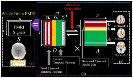
In this paper, we propose a novel supervised sparse representation and dictionary learning framework, named supervised stochastic coordinate coding (SCC), for task fMRI data analysis, in which certain brain networks are learned with known information such as pre-defined temporal features and spatial network patterns, and at the same time other concurrent networks are learned automatically from data. The proposed method takes advantages of both hypothesis-driven methodology and data-driven methodology for fMRI analysis.

1. INTRODUCTION

Task functional magnetic resonance imaging (fMRI) has been well established for mapping brain activations and network activities (Logothetis 2008; Friston et al., 1994). It is widely believed that rich information is hidden in task fMRI data, but how to effectively mine them out has been challenging because of the intrinsic complexity (Logothetis 2008; Heeger and Ress, 2002; Kanwisher et al., 2010; Duncan et al., 2010). Among all state-of-the-art methodologies, the general linear model (GLM) has been the dominant approach in detecting functional networks from task fMRI data (Friston et al., 1994) by regressing the designed task pattern from fMRI signals. However, the simple task design patterns are limited in detecting the diverse brain networks that are participating in the task or maintaining consciousness (Bullmore & Sporns, 2009; Duncan et al., 2010). In addition, many human neuroscience studies have widely reported and argued that a variety of cortical brain regions and networks exhibit strong functional diversity (Duncan et al., 2010; Gazzangia et al., 2004; Pessoa et al., 2012), that is, certain cortical regions could participate in multiple functional networks or processes and a functional network might recruit various heterogeneous neuroanatomic areas (Duncan et al., 2010; Gazzangia et al., 2004). Therefore, the traditional hypothesis-driven methods such as GLM are limited in inferring those concurrent networks because they are likely to overlook the heterogeneous regions and diverse activities participating in a task performance (Logothetis 2008; Duncan et al., 2010). Consequently, they are not likely to be sufficient in exploring concurrent, particularly heterogeneous, task-evoked functional networks and assessing systematic brain-wide activities during task performance.

Recently, dictionary learning and sparse representation methodology developed in the machine learning field has been shown to be efficient in learning adaptive, over-complete and diverse features for optimal representations (Mairal et al., 2010; Wright et al., 2009; Lin et al., 2014). Earlier works that adopted sparse representation in fMRI data analysis showed promising performance (Lv et al., 2015a; Lv et al., 2015b; Lv et al., 2015c; Lee and Ye, 2011). The basic idea is to aggregate all the hundreds of thousands of task fMRI signals within the whole-brain of one subject into a big data sample pool, based on which an over-complete dictionary and a sparse code matrix for optimal representation will be learned via dictionary learning and sparse coding algorithms (Lv et al., 2015a; Lv et al., 2015b; Mairal et al., 2010). Particularly, the signal shape of each dictionary atom represents the functional activities of a specific brain network and its corresponding sparse code vector among all the voxels can be reorganized back in brain volumes as the spatial distribution of this specific brain network (Lv et al., 2015a; Lv et al., 2015b). An important characteristic of this framework is that concurrent brain networks that are captured by task fMRI images and signals can be reconstructed simultaneously in an automatic way. This data-driven strategy naturally accounts for the fact that each brain region could be involved in multiple concurrent functional processes (Duncan et al., 2010; Gazzangia et al., 2004; Pessoa et al., 2012) and thus its signal is composed of various heterogeneous components (Lv et al., 2015a; Lv et al., 2015b; Lee et al. 2011). In the work of Lv et al., 2015a and Lv et al., 2015b, task-evoked networks could be effectively learned from task fMRI data, as well as all the well-established intrinsic networks (Smith et al., 2009), which are usually modeled in resting state fMRI data (Lv et al., 2015a; Lv et al., 2015b). This provides new clues for the architecture of functional brain networks. However, because of the data-driven strategy used, the learned task evoked networks might be affected by noise and identifying the intrinsic networks from all the learned components could be difficult and ambiguous (Lv et al., 2015a; Lv et al., 2015b).

Therefore, adopting the dictionary learning and sparse representation method into neuroscience applications entails a novel, flexible framework that can guide or supervise the learning procedure with task design and/or neuroscience knowledge. Typically, the design of task paradigms provides useful information about the temporal feature in the signals. Meanwhile, prior neuroscience knowledge could be used to constrain spatial patterns of the inference such as network templates or brain mapping atlases. Therefore, if prior knowledge about the temporal feature and spatial signatures could be incorporated into the dictionary learning, we could effectively integrate hypothesis-driven and data-driven methods and maximize the benefits of both strategies. To achieve this goal, we here propose an innovative supervised sparse dictionary learning framework for task fMRI data analysis based on stochastic coordinate coding (SCC: http://www.public.asu.edu/~jye02/Software/SCC/) (Lin et al., 2014). On one hand, our method could constrain temporal features such as task designs as part of learned dictionary in order to map the spatial distribution of these features. On the other hand, we could supervise the dictionary atom signal learning with known spatial patterns such as network templates. Thus, we call it supervised SCC. With the supervised SCC method, meaningful task evoked networks and well-established intrinsic networks can be inferred with known temporal and spatial features, and at the same time, other concurrent networks can be learned simultaneously and automatically from the data. We then performed extensive qualitative and quantitative evaluations to demonstrate that our method provides a new and effective framework for task fMRI data analysis.

2. METHODS

2.1 Overview

Our supervised stochastic coordinate coding (SCC) framework for task fMRI data modeling is summarized in Fig. 1. Briefly, fMRI signals extracted from a brain mask can be organized into a signal matrix S (Fig. 1a). The original SCC method will then learn a temporal basis dictionary matrix D containing the most representative activities in the brain from the signal matrix S. And at the same time a sparse code matrix A (Fig. 1b) which structures the spatial organization of the brain activities are learned with sparsity constraints. In other words, the learning process will preserve the organization of signals of voxels so that each row in A can be mapped back to brain volume, which we call a brain network as shown in Fig. 1c. The SCC can be supervised with fixed temporal features in D and constrained spatial features in A as shown in Fig. 1b. Specifically, in our supervised SCC, temporal features such as task designs can be fixed in D as D_C and they keep unchanged during the whole training. Accordingly, the rows in A_C are learned spatial distributions of D_C atoms. Based on our innovation of the SCC method in solving sparse coding problem, we can restrict the spatial patterns of networks in A_R, correspondingly, and we can also learn the major signal contribution in D_R of the restricted spatial patterns. Along with the temporal constraint and spatial restrictions, the rest part of D and A, i.e. D_l and A_l, will be learned automatically in a data-driven way so that the diversity of concurrent brain networks could be modeled. More details will be discussed in the following sections. And explanations of variables could be found in Supplemental Table. 1.

Fig. 1.

Illustration of the framework of supervised stochastic coordinate coding (SCC) for task fMRI data modeling. (a) FMRI signals in the brain mask are extracted and organized into a signal matrix S. (b) S is decomposed into a dictionary matrix D and a sparse code matrix A by the supervised SCC. D_C: Fixed dictionary atoms. D_R: learned dictionary atoms for constrained spatial patterns. D_l: Automatically learned dictionary atoms. A_C: learned spatial maps corresponding to D_C. A_R: Restricted spatial maps while learning. A_l: Automatically learned concurrent networks. (c) Each row of A can be mapped back to brain volume as a spatial network.

2.2 Stochastic Coordinate Coding of FMRI Data

2.2.1 Background and Problem Formulation

In the task fMRI data, signals are organized with voxel locations. Considering each fMRI signal from a voxel as a learning sample, the pool of signals within the brain mask is represented as S = [s₁ … … s_n]εℝ^t×n, in which t is the number of time points in each signal and n is the voxel number in the brain mask. The aim of the sparse coding is to learn a dictionary of signal basis Dεℝ^t×m from the signal pool, and a sparse code matrix Aεℝ^m×n, so that S is modeled as a sparse linear combination of atoms of a learned basis dictionary D, i.e., s_i = Da_i or written as S=DA (Mairal et al., 2010; Lv et al., 2015a; Lv et al., 2015b). The reconstruction error is required to be minimized and it is further assumed that each input signal can be represented only by a small group of dictionary atoms, that is, sparsity is constrained. In this way, the temporal features in the dictionary can be optimally selected and efficiently coded to represent each training sample.

Then, given the signal s_i, the above idea can be formularized as an optimization problem:

$$\mathit{min}{f}_i(D,a_i)=\mathit{min}\frac{1}{2}{\Vert s_i-D{a}_i\Vert }^2+\lambda {\Vert a_i\Vert }_1,$$ (1)

in which both D and a_i need to be learned and λ is the regularization parameter. In order to prevent arbitrary scaling of the sparse code, each sample s_i is normalized before training and each column of D is restricted to be in a unit ball, i.e., ||d_j|| ≤ 1 during training. Given the whole-brain data set S, the minimization function is summarized as follow:

$$\underset{D\in B_m,a_1,\dots a_n}{min}F(D,a_1,\dots a_n)\equiv \frac{1}{n}\sum _{i=1}^n{f}_i(D,a_i)$$ (2)

where D is restricted with the normalization procedure iteratively as follows:

$$B_m=\{D\in {ℝ}^{\mathrm{t}\times \mathrm{m}}:\forall j=1,\dots ,m,{\Vert d_j\Vert }_2\le 1\}$$ (3)

The above problem is non-convex with respect of joint parameters of D and A = [a₁, … a_n]. But it is a convex problem when either D or A is fixed. Specifically, when D is fixed, solving each sparse code a_i is the well-known LASSO problem (Tibshirani et al., 1996), while if A is fixed it’s a simple quadratic problem. Therefore, alternating optimization approach is usually adopted to solve the above sparse coding problem. The traditional alternating method is usually summarized in the following way:

1. Get an input sample s_i.

2. Calculate the sparse code a_i by using LARS (Efron et al., 2004), FISTA (Beck et al., 2009) or coordinate descent (Wu and Lange, 2008).

3. Update the dictionary D by performing stochastic gradient descent.

4. Go to step 1 and iterate.

2.2.2 Stochastic Coordinate Coding

In the stochastic coordinate coding (SCC: http://www.public.asu.edu/~jye02/Software/SCC/) method (Lin et al., 2014), the same strategy was adopted as mentioned in the Section 2.2.1, but with significant innovation in updating a_i and D (Lin et al., 2014), which makes the method much more efficient in dealing with big fMRI data. Details will be discussed in the following paragraphs.

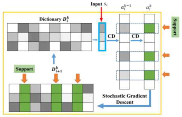
Some concepts are firstly defined for the method to be better illustrated. In the method, each a_i is called sparse code. Since a_i is sparse, only a few entries in a_i are non-zero. The non-zero entries of a_i are defined as its support, i.e., support (a_i)={ 1, if a_i,j ≠ 0; 0, if a_i,j = 0. (j = 1, …, m)}ε {0,1}^m×1. The support will be a screen that guides necessary and efficient updating of a_i and D. The training process will take a few cycles on the whole data set, and each cycle, i.e., each input signal in S has been trained once, is called as an epoch. In the following sections, superscript k will be used to represent the number of epochs and subscript i will be used to represent the index of data samples. Note that another innovation of the method is that the approximation of the inverse of Hessian matrix of the objective function is used to define the learning rate of gradient descent. In this way, manually tuning the learning rate parameter is avoided (Wu and Lange, 2008). Specially, the matrix $H={\mathrm{\sum }}_{k,i}{a}_i^k{(a_i^k)}^T$, is an approximation of the Hessian when k and i go to infinity in the step 2 of Algorithm 2. The SCC algorithm is detailed as follows.

Initialize the dictionary via any initialization method, such as random weights, random patches or k-means (Jarrett et al., 2009). And denote it as $D_1^1({ℝ}^{t\times m})$, Initialize the sparse code $a_i^0=0({ℝ}^{m\times 1})$, for i=1,…, n, support ( $a_i^0$) is all zero. H is initialized as 0. Then starting from k=1 and i=1:

1. Get an input sample s_i.

2. Update $a_i^k$ with Algorithm 1.

3. Update the dictionary D with Algorithm 2.

4. i = i + 1. If i > n, then set $D_1^{k+1}=D_{n+1}^k$, k= k + 1 and i = 1. Go to step 1.

Algorithm 1.

Update $a_i^k$.

1.	Perform a few steps of Coordinate Descent (CD) until the locations of non-zero entries achieve stability:
	$$a_i^{k-1}=CD({\mathrm{D}}_{\mathrm{i}}^{\mathrm{k}},a_i^{k-1},{\mathrm{s}}_i)$$ (4)
	One step of coordinate descent:
	for j=1 to m do
	$$b_j\leftarrow {(d_{i,j}^k)}^T(s_i-D_i^k{a}_i^{k-1})+a_{i,j}^{k-1},$$ (5)
	$$a_{i,j}^{k-1}\leftarrow h_{\lambda }(b_j),$$ (6)
	end for
2.	Update support ( $a_i^{k-1}$).
3.	Update $a_i^k$ with certain number of coordinate descent on the support:
	One step of coordinate descent on the support:
	for j=1 to m do
	if support $(a_i^{k-1})(j)=1$ do
	$$b_j\leftarrow {\left(d_{i,j}^k\right)}^T\left(s_i-D_i^k{a}_i^{k-1}\right)+a_{i,j}^{k-1},$$ (7)
	$$a_{i,j}^{k-1}\leftarrow h_{\lambda }(b_j),$$ (8)
	end if
	end for
4.	$a_{i,j}^k\leftarrow a_{i,j}^{k-1}$

The four steps are conceptually illustrated in Fig. 2 and details are demonstrated in Algorithm 1 and Algorithm 2. In Algorithm 1, updating $a_i^k$ is the classical LASSO problem, in which it usually takes tens of hundreds of steps to converge. But as reported in Lin et al., 2014, the support of the coordinates, i.e., the location of the non-zero entries will keep accurate after only a few steps. Thus, the algorithm firstly takes a few steps of coordinate descent to fully update the vector $a_i^k$ until the locations of non-zero entries achieve stability, and in this way the Support ( $a_i^k$) will be determined. As a result, the next steps of coordinate descent will only focus on updating $a_i^k$ on the support (Fig. 2), which will save much computing time. Note that Support $(a_i^{k-1})(j)$ denotes the j-th value in the vector of Support ( $a_i^{k-1}$). And while applying the L1 norm, the soft shrinking function is defined as follow:

$$h_{\lambda }(v)=\{\begin{array}{cc}v+\lambda ,& v<-\lambda \\ 0,& -\lambda \le v\le \lambda \\ v-\lambda ,& v>\lambda \end{array}$$ (9)

Fig. 2.

Illustration of the mechanism of updating coefficients and dictionary in the Stochastic Coordinate Coding method. The support is defined by a binary screen to guide the updating (Lin et al., 2014). CD stands for Coordinate Descent.

Algorithm 2.

Update D

1.	Update support ( $a_i^k$).
2.	$H\leftarrow H+a_i^k{(a_i^k)}^T,{\eta }_{i,j}^k=1/h_{jj}$
3.	Update the dictionary D by using stochastic gradient descent:
	$$D_{i+1}^k=P_{B_m}(D_i^k-{\eta }_i^k{\nabla }_{D_i^k}{f}_i(D_i^k,a_i^k))$$ (10)
	$${\nabla }_{D_i^k}{f}_i\left(D_i^k,a_i^k\right)=(D_i^k{a}_i^k-s_i){(a_i^k)}^T$$ (11)
	One step of stochastic gradient descent:.
	for j=1 to m do
	if support $(a_i^{k-1})(j)=1$ do
	$$d_{i+1,j}^k\leftarrow d_{i,j}^k-{\eta }_{i,j}^k{a}_{i,j}(D_i^k{a}_i^k-s_i)$$ (12)
	end if
	end for

^*P_Bm means applying the B_m constraint defined in Eq.3.

In Algorithm 2, suppose that $a_{i,j}^k=0$, then ${\nabla }_{d_{i,j}^k}{f}_i\left(D_i^k,a_i^k\right)=(D_i^k{a}_i^k-s_i){(a_{i,j}^k)}^T=0$, therefore $d_{i,j}^k$ dose not need to be updated, which saves a lot of computing and is the advantage of SCC (Lin et al., 2014).

2.3 Fixing Temporal Features in Stochastic Coordinate Coding

When modeling the task fMRI data, the exterior paradigm designs are usually summarized as the design matrix, which is a set of time series that is coded with stimulus knowledge. In the traditional GLM method, these time series are used as explanatory variables of the real fMRI data for activation detection. In our method, we normalize these task designs into the B_m constraint (Eq.3) and set them as the dictionary of stochastic coordinate coding or part of the dictionary.

If the task designs are treated fully as a fixed dictionary D, the problem becomes easier because it turns into a LASSO problem, as discussed in Section 2.2.1. But if we only fix the task designs as part of the dictionary, the dictionary will be composed of a constant part D_c and a learned part D_l.

$$D=[{\mathbf{D}}_{\mathrm{c}},D_l]\epsilon {ℝ}^{t\times m},{\mathbf{D}}_{\mathrm{c}}\epsilon {ℝ}^{t\times m_c},D_l\epsilon {ℝ}^{t\times m_l}$$

Then the optimization function turns into Eq.13.

$$\mathit{min}{f}_i([{\mathbf{D}}_{\mathrm{c}},D_l],a_i)=\mathit{min}\frac{1}{2}{\Vert s_i-[{\mathbf{D}}_{\mathrm{c}},D_l]a_i\Vert }^2+\lambda {\Vert a_i\Vert }_1$$ (13)

The alternative updating of D and a_i still works on this non-convex problem. The only difference is that Eq.10 will turn to Eq.14.

$${[{\mathbf{D}}_{\mathrm{c}},D_l]}_{i+1}^k=P_{B_m}({[{\mathbf{D}}_{\mathrm{c}},D_l]}_i^k-{\mathrm{\eta }}_i^k{\nabla }_{D_i^k}{f}_i({[{\mathbf{D}}_{\mathrm{c}},D_l]}_i^k,a_i^k))$$ (14)

In Algorithm 2, the updating process will jump over the constant dictionary part but only update the learned part. However, during each iteration the sparse code of the whole dictionary including D_c and D_l will update accordingly. In this way, we will find the contribution of the task designs on each voxel, and in a global view we will find the distribution of the task designs on the brain volume.

2.4 Minimizing Intra-correlation in the Learned Dictionary

In the previous section, D_c is fixed in the dictionary learning, while D_l is automatically learned. However, because the task designs are usually ideally hypothesized signal patterns without any noise considered as shown in Fig. 4 and Fig. 5, based on our experience it would be possible that a few atoms in D_l are correlated with D_c, which we call intra-correlation of the dictionary atoms. The intra-correlation will potentially affect the detection of task-evoked networks, so that we propose to minimize it while learning the entire dictionary. In order to minimize the intra-correlation, we introduce a new term to Eq.13 as shown in Eq.15.

Fig. 4.

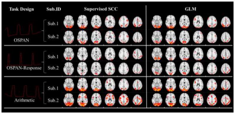
The task-related networks in two single subjects in the working memory task detected by fixing task designs in the dictionary. First column: Fixed task designs. Second column: Subject IDs. For each task design we visualized results from two randomly selected subjects. Third column: Learned spatial patterns of the supervised SCC method. Fourth column: Activation maps (Threshold: z>2.3) detected by the GLM method for comparison.

Fig. 5.

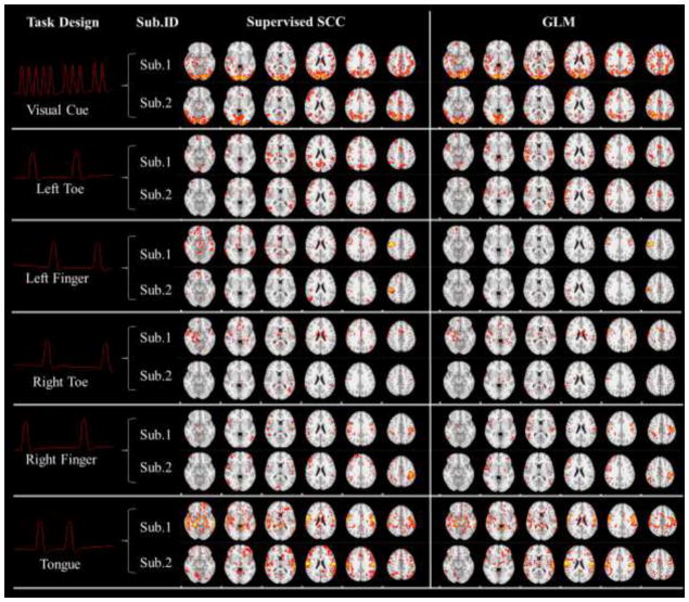
The task-related networks of two single subjects in the motor task detected by fixing task designs in the dictionary. First column: Fixed task designs. Second column: Subject IDs. For each task design we visualized results from two randomly selected subjects. Third column: Learned spatial patterns of the supervised SCC method. Fourth column: Activation maps (Threshold: z>2.3) detected by the GLM method for comparison.

$$\mathit{min}{f}_i([{\mathbf{D}}_{\mathbf{c}},D_l],A)=\mathit{min}\frac{1}{2}{\Vert s_i-[{\mathbf{D}}_{\mathrm{c}},D_l]a_i\Vert }^2+\lambda {\Vert a_i\Vert }_1+\frac{1}{2}\gamma {\Vert {\mathbf{D}}_{\mathbf{c}}^{\mathrm{T}}{D}_l\Vert }_F^2,$$ (15)

where the second term $\frac{1}{2}\gamma {\Vert {\mathbf{D}}_{\mathbf{c}}^{\mathrm{T}}{D}_l\Vert }_F^2$ ensures the low correlation between D_c and D_l. The updating rule of D_l should be changed accordingly. Basically, when performing stochastic gradient descent, there will be a new term in the gradient of D_l, i.e. Eq.12 will be written as Eq.16. And note that in the whole learning procedure, the D_c will keep unchanged as initialized.

$${\nabla }_{{[D_l]}_i^k}{f}_i\left(D_i^k,a_i^k\right)=\left({[{\mathbf{D}}_{\mathrm{c}},D_l]}_i^k{a}_i^k-s_i\right){\left(a_i^k\right)}^T+\gamma {\mathbf{D}}_{\mathbf{c}}{\mathbf{D}}_{\mathbf{c}}^{\mathrm{T}}{[D_l]}_i^k$$ (16)

2.5 Constraining Spatial Maps in Stochastic Coordinate Coding

In neuroscience, atlases or interested networks are usually defined in the spatial domain, such as the default mode network (DMN), executive control network and auditory network, and etc. So it will be interesting to investigate what is the major signal pattern in a certain interested region or network. The premise is as follows. The signal set S = [s₁, … s_n]εℝ^t×n is a collection of fMRI signals of voxels within the brain mask. They are extracted with a certain principle, and the SCC method will preserve the principle, i.e., the order of voxels, in the learned sparse code matrix A = [a₁, … a_n] εℝ^m×n. In this way, if we map each row of the sparse code back following the principle of signal extraction, there will be m spatial maps which correspond to the distributions of m dictionary atom signals. We call these spatial maps as interested brain networks (Lv et al., 2015a; Lv et al., 2015b).

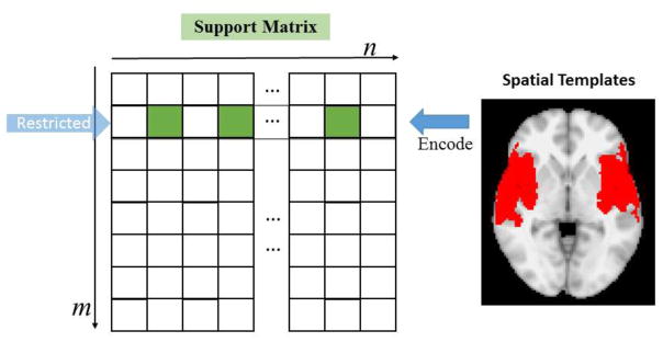
In this section, we will adjust the SCC by restricting certain rows of the support matrix of A with the spatial distribution information, as illustrated in Fig. 3. Suppose we have an interested spatial pattern within the brain mask, the pattern itself is labeled by 1, and the rest of brain mask is labeled by 0. Then the pattern can be represented as a binary vector Vε{0,1}^1×n with the same voxel organization of A. We set the pattern as constraint of the p-th row of A, so that support(a_i)(p)=V(i), for i = 1, …, n. After the support of each voxel at the p-th row is set at the initialization, they will keep unchanged during the whole training procedure, and the updating of A on this row will only happen on the non-zero part of the support.

Fig. 3.

Illustration of restricting spatial templates by defining support on a certain row. The binary spatial map will be encoded in the support matrix as a row. Updates will only happen on the green entries of the row.

Since the support of the p-th row was predefined while the supports of the other rows are initialized with 0, a regularization will be made before the updating of $a_i^{k-1}$, that is, if j=p the Eq.6 turns to Eq.17.

$$a_{i,p}^{k-1}\leftarrow \{\begin{array}{c}0,\mathit{support}\left(a_i^{k-1}\right)(p)=0\\ h_{\lambda }\left(b_j\right),\mathit{support}\left(a_i^{k-1}\right)(p)=1\end{array}$$ (17)

Note that, in Eq.17, if the shrinking function h_λ(b_j) returns 0 in a certain iteration, we will update $a_{i,p}^{k-1}$ as an infinite small value, such as 1×10⁻⁴. In following step of Algorithm 1 and Algorithm 2, we make sure the support of a_i at the p-th row keep the same as what is initialized. And in future analysis of the spatial map, the voxels with value of 1×10⁻⁴ will not be considered because they are supposed to be zero. With the help of restriction on the support, we can learn the major signal contributions and their strength distributions in the interested brain region or network.

2.6 Group-wise Statistical Analysis of Network Spatial Maps

Individual variability widely exists in the learned network spatial maps. Similar to the statistical parameter mapping (SPM) (Friston et al., 1994), we can also perform group-wise statistical analysis on the spatially normalized networks across subjects with the correspondences established by D_C and A_R. In this paper, all data are registered into the MNI atlas space before applying our method, and null hypothesis t-test was applied to generate group-wise statistical z-score maps for each corresponding network in A_C and A_R. This is one major advantage relative to the data-driven method in (Lv et al., 2015a; Lv et al., 2015b), because task networks and intrinsic networks could easily be identified in each individual and statistically assessed across populations.

However, there are still many learned concurrent networks in A_l which are learned automatically without any prior correspondence settled. Thus, we employ K-means clustering method to find networks which possess spatial pattern similarity among subjects, i.e., these networks consistently exist across subjects with similar spatial patterns. In this way, correspondence of automatically learned networks could also be roughly established.

3. RESULTS

We evaluated our method on two independent task fMRI datasets. These two datasets are described in Section 3.1. Then the following sections examine task-evoked networks inferred by fixing temporal features (Section 3.2), motion components modeled by supervised SCC (Section 3.3), the effects of minimizing intra-correlation (Section 3.4), the networks detected by restricting spatial templates (Section 3.5), automatically learned networks from data (Section 3.6), and the influence of parameter selection (Section 3.7). The results in Section 3.2, Section 3.3, Section 3.5 and Section 3.6 are generated based on the setting of dictionary size as 200, λ=0.16 and γ= 2×10⁻³ for both data sets.

3.1 FMRI Data and Preprocessing

Working Memory (WM) task dataset

This dataset were acquired on a 3T GE Signa scanner at the University of Georgia under IRB approval (Faraco et al., 2011). Here, 28 subjects performed an operational span (OSPAN) working memory task while fMRI data was acquired. Acquisition parameters are as follow: 64×64 matrix, 4mm slice thickness, 220mm FOV, 30 slices, TR=1.5s, TE=25ms, ASSET=2. Each participant performed a modified version of the OSPAN task (4 block types: OSPAN, OSPAN response, Arithmetic, and Baseline). For more detail of data collection please refer to (Faraco et al., 2011). And the block designs of the task are visualized as the red curves in Fig. 4.

Motor task dataset

In the human connectome project (HCP) Q1 data set (Barch et al., 2013), a motor task fMRI dataset was acquired for 68 subjects. The acquisition parameters of fMRI data are: 90×104 matrix, 220mm FOV, 72 slices, TR=0.72s, TE=33.1ms, flip angle = 52°, BW =2290 Hz/Px, in-plane FOV = 208 × 180 mm, 2.0 mm isotropic voxels. Six different stimulus designs, including visual cues and movements of left toe, left finger, right toe, right finger and tongue are alternated in different blocks. The block designs of the task are visualized as the red curves in Fig. 5.

The preprocessing pipeline includes motion correction, slice time correction, spatial smoothing and high-pass filtering. After pre-processing the fMRI data of all subjects are registered to the MNI space with the non-linear registration tool FSL FNIRT (Andersson et al., 2010), and for better registration accuracy the high resolution structure images were used to guide the registration. Whole brain signals of each subject were extracted voxel by voxel and arranged into a signal matrix, and each signal are normalized with mean of 0 and standard deviation of 1.

3.2 Detecting Task-evoked Networks using Supervised SCC

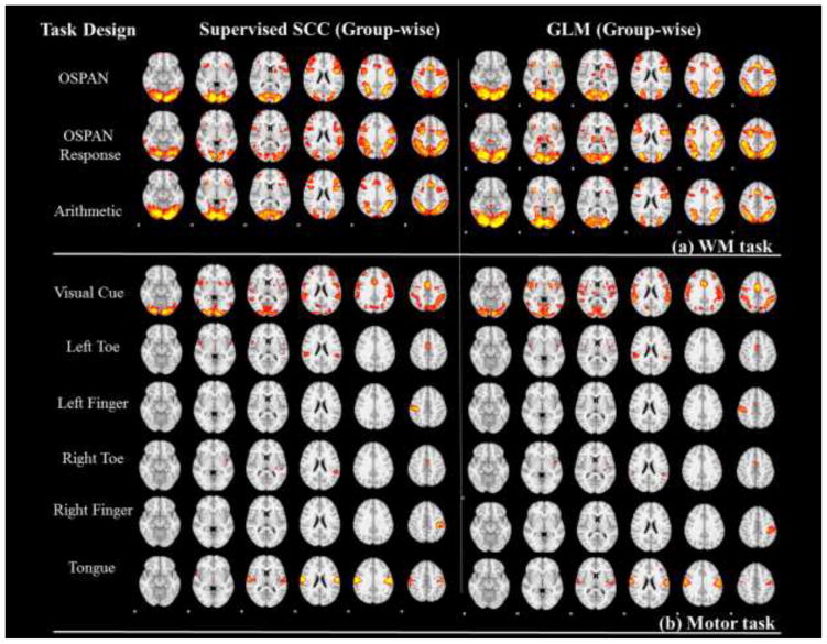
The block-designed stimuli in Section 3.1 are set as the fixed temporal features in our supervised SCC method. These task designs are firstly convolved with hemodynamic response function (HRF) before the training, as shown in the first column of Fig. 4 and Fig. 5. The results from the supervised SCC in this section are based on the setting of minimization of intra-correlation in Section 2.4, and parameter λ was set so that the learned task evoked networks exhibit the similar level of noise to GLM activations. The discussion about the effects of intra-correlation minimization is in Section 3.4. For comparison, the same designs are also set as explanatory variables of GLM based method with FSL FEAT (http://fsl.fmrib.ox.ac.uk/fsl/fslwiki/FEAT). We compared the results from the two methods at both the single subject level and at group level. Specifically, in Fig. 4 and Fig. 5, we show the task-evoked networks of two randomly selected subjects using either the supervised SCC or the GLM based method. From the comparison, we found that spatial patterns were quite similar from both methods. This observation is consistent across different subjects. After applying the statistical analysis in Section 2.6, group-wise statistical maps are compared with group-wise activation from FEAT (Beckmann et al., 2003) in Fig. 6. The results are also very similar between two methods, although variation exists because of algorithm difference and parameter settings. Quantitatively, we used the Dice’s coefficients to measure the similarity of the group-wise results and found high similarity (Table. 1 and Table. 2). Thus, our supervised SCC method is comparable with GLM in detecting task-evoked activations or networks.

Fig. 6.

Group-wise statistical z-score maps from Supervised SCC method and GLM method (Threshold: z>6.5). The task designs are corresponding to Fig. 2. (a) Group-wise maps from working memory task; (b) Group-wise maps from the motor task.

Table 1.

The Dice’s coefficients of group-wise task-evoked networks from two methods (supervised SCC and GLM) in the Working Memory task.

WM Task	OSPAN	OSPAN Response	Arithmetic
Dice’ Coefficient	0.82	0.80	0.83

Table 2.

The Dice’s coefficients of group-wise task-evoked networks from two methods (supervised SCC and GLM) in the Motor task.

Motor Task	Visual Cue	Left Toe	Left Finger	Right Toe	Right Finger	Toe
Dice’ Coefficient	0.91	0.71	0.70	0.70	0.64	0.77

3.3 The Motion Components Modeled by Supervised SCC

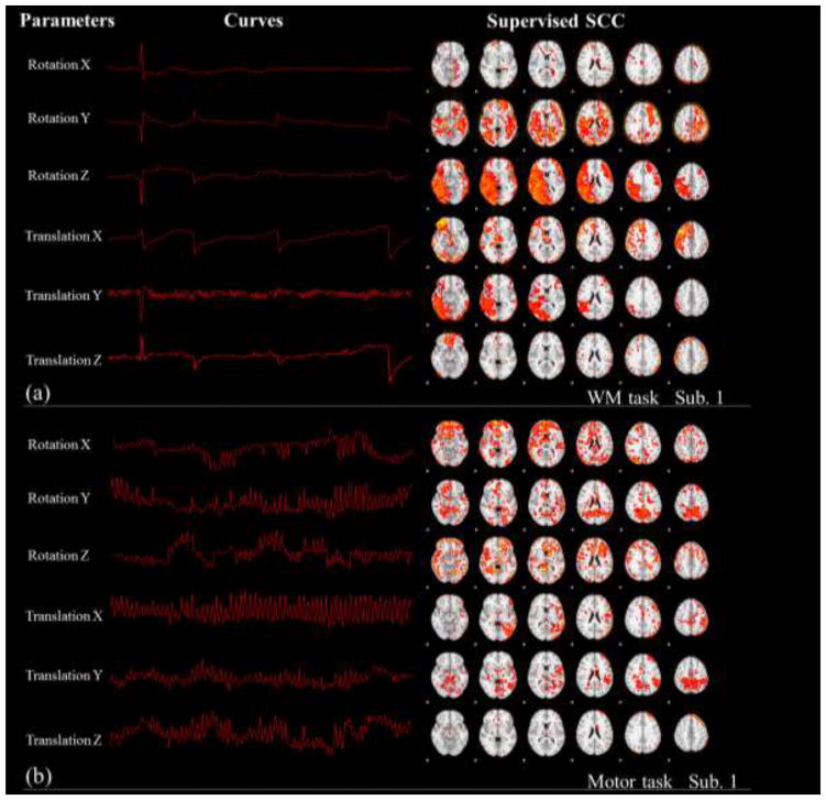
Motion correction is a crucial step in fMRI analysis to remove the artifacts caused by head motion. However, even after motion correction there are still residual effects of motion left in the data (Jenkinson et al., 2002). In the GLM based method like FSL FEAT, the motion parameters estimated from data are usually set as confound explanatory variables (Friston et al., 1994). In our supervised SCC method, similar as Section 3.2, we set the six motion parameters estimated from motion correction (Jenkinson et al., 2002) as part of the fixed dictionary D_c, and two exemplar results from both data sets are shown in Fig. 7. In Fig. 7, by mapping the corresponding coefficients back to the brain volume, we could visualize the effect strength of motion on each voxel. By minimizing the intra-correlation between the motion parameters and other dictionary atoms with the setting in Section 2.4, the head motion artifacts could be minimized while modeling other brain networks in the dictionary learning. Quantitatively, without fixing motion parameters, the average Pearson’s correlation between the motion parameters and the dictionary atoms learned is relatively high, indicating the impact from head motion (the second row of Table. 3 and Table. 4). In contrast, by setting the motion parameters as part of the fixed dictionary, the correlation between motion atoms and other atoms are significantly (about 1000 times) reduced (the third row of Table. 3 and Table. 4). In this way, we can substantially improve the quality of the reconstructed networks by minimizing the motion effects.

Fig. 7.

The spatial patterns learned from the Supervised SCC method by fixing the motion parameters. Results of one subject from the working memory and motor task are visualized, respectively. The second column shows the motion patterns from each subject and the third column shows the spatial maps learned from Supervised SCC.

Table 3.

The average correlation between motion parameters and the learned dictionary atoms in the working memory task. “Not Set” means “not set motion parameters as fixed part of the dictionary”. “Set” means “set motion parameters as fixed part of the dictionary”.

WM Task	Rotation X	Rotation Y	Rotation Z	Translation X	Translation Y	Translation Z
Not Set	0.22	0.29	0.23	0.30	0.19	0.31
Set	0.00013	0.00025	0.00010	0.00057	0.00009	0.00054

Table 4.

The average correlation between motion parameters and the learned dictionary atoms in the Motor task. “Not Set” means “not set motion parameters as fixed part of the dictionary”. “Set” means “set motion parameters as fixed part of the dictionary”.

Motor Task	Rotation X	Rotation Y	Rotation Z	Translation X	Translation Y	Translation Z
Not Set	0.19	0.21	0.24	0.21	0.20	0.17
Set	0.00036	0.00038	0.00022	0.00033	0.00026	0.00021

3.4 The Effects of Minimizing the Intra-correlation

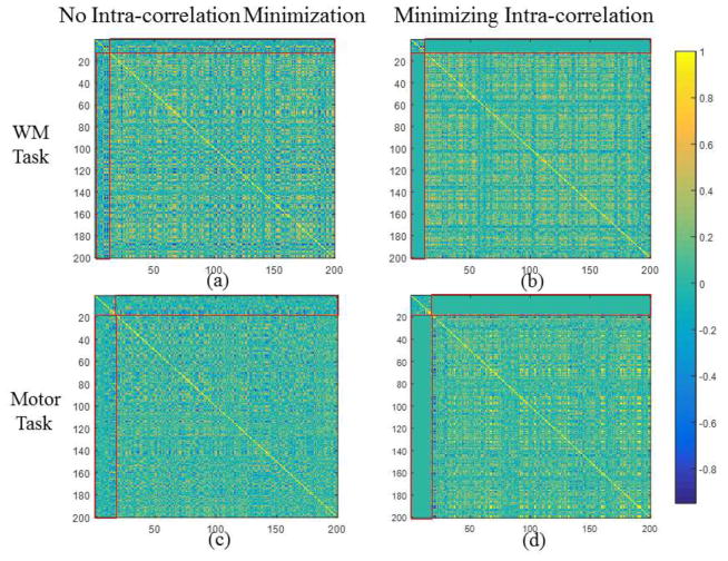
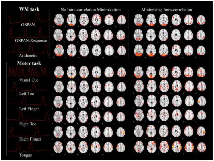
The stochastic coordinate coding method itself employs L1 penalty to regularize the dictionary learning, i.e., the sparsity is the rule of representing fMRI signals, which coincide with the intrinsic organization of neurons (Olshausen, 1996; Olshausen and Field, 2004). However, although the dictionary is learned with optimized differences among atoms, the correlation among them are not minimized. As a consequence, when we set the designed task paradigms as the fixed part of the learned dictionary, there is a chance that the noise-free paradigm will not be selected or weakly selected while alternative atoms will be learned out in the D_l part. This will cause uncertainty to the detection of task-related networks. For example, in Table. 5 and Table. 6, before minimizing the intra-correlation, we could possibly learn other dictionary atoms with high correlation (maximally 0.77) with task designs. Hence we propose to minimize the intra-correlation in Section 2.4, through which the task-evoked networks will be concentrated in the D_c and A_c part. Here we introduce the tunable parameter γ to regularize the minimization. As shown in Fig. 8, we compared the correlation matrix of the learned dictionary with γ=0 and γ=0.02. As highlighted by the red block in Fig. 8, the absolute values of correlations between D_c and D_l for both tasks are significantly reduced after turning on the minimization. Quantitatively, we measured the maximum correlation between the task designs and other learned atoms with and without intra-correlation minimization in Table. 5 and Table. 6. From the comparisons in Table. 5 and Table. 6, we can infer that with the minimization of intra-correlation, the learned atoms exhibit quite low correlation (around 10⁻³) with task designs, so that the task-related networks are concentrated in the D_c and A_c part. In addition, corresponding A_c with both settings are mapped back to brain volume for comparison, as shown in Fig. 9. By comparing the second and third column of Fig. 9, it’s quite obvious that after turning on the intra-correlation minimization, the task-evoked networks are enhanced. We also quantitatively compared the voxel number of task-evoked networks with and without intra-correlation minimization in Table. 7 and Table. 8, and found that with intra-correlation minimization, the task networks are enlarged 1.5~2.5 times. In summary, by using the intra-correlation minimization, the task-evoked networks could be significantly enhanced. The selection of γ is further discussed in Section 3.7.

Table 5.

The maximum correlation between task designs and other learned dictionary atoms in the Working Memory task. “With” means “with minimizing intra-class correlation”. “Without” means “without minimizing intra-class correlation”.

WM Task	OSPAN	OSPAN Response	Arithmetic
Without	0.49	0.48	0.40
With	0.0010	0.0017	0.00056

Table 6.

The maximum correlation between task designs and other learned dictionary atoms in the Motor task. “With” means “with minimizing intra-class correlation”. “Without” means “without minimizing intra-class correlation”.

Motor Task	Visual Cue	Left Toe	Left Finger	Right Toe	Right Finger	Toe
Without	0.39	0.42	0.52	0.50	0.48	0.77
With	0.0014	0.0015	0.0020	0.0013	0.0016	0.0016

Fig. 8.

The comparison of correlation matrix of learned dictionary with and without minimization of intra-correlation. (a) and (b) are for the working memory task. (c) and (d) are for the motor task.

Fig. 9.

The effects of minimization of intra-correlation on the learned task related networks. The first column shows the task designs from both the working memory task and motor task. The second column shows the results without intra-correlation minimization from one single subject of each task. And the third column shows the results with intra-correlation minimization from one single subject of each task.

Table 7.

The voxel number of the detected task-evoked networks in the working memory task. With” means “with minimizing intra-class correlation”. “Without” means “without minimizing intra-class correlation”.

WM Task	OSPAN	OSPAN Response	Arithmetic
Without	12366	5748	21464
With	37649	12187	35436

Table 8.

The voxel number of the detected task-evoked networks in the motor task. With” means “with minimizing intra-class correlation”. “Without” means “without minimizing intra-class correlation”.

Motor Task	Visual Cue	Left Toe	Left Finger	Right Toe	Right Finger	Toe
Without	14771	8437	9942	15555	9088	10936
With	20223	15236	15647	22431	15428	16258

3.5 Networks Detected by Restriction of Spatial Maps

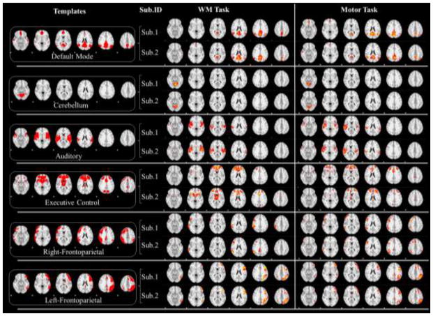
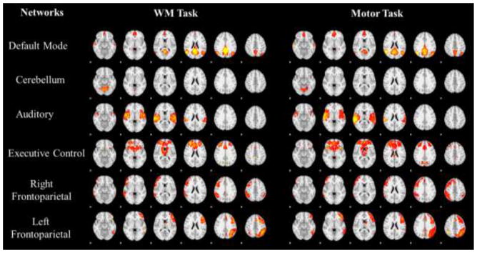
With our method, we could also set the well-established brain network templates (like the default mode network (DMN), auditory network, executive control network etc.) (Smith et al., 2009), which are believed to function in different brains and across different tasks (Smith et al., 2009; Lv et al., 2015a; Lv et al., 2015b), as spatial restrictions while learning dictionaries. As shown in the first column of Fig. 10, we selected 6 networks for this experiment, and the red regions are the constrained regions in which the updating of temporal patterns and sparse codes take place. The learning results of both working memory task and motor task are visualized for two random subjects (second and third column of Fig. 10), showing that there are reasonable Gaussian-like distributions in the restricted regions. Note that certain regions are valued with 1×10⁻⁴: these regions are supposed to be zero according to our algorithm in Section 2.5 and were dropped from our results because the difference across subjects turns out to account for the individual variability of the same network. And we further perform group-wise statistical t-test as illustrated in Section 2.6, and the group-wise networks by spatial restriction are shown in Fig. 11. The distributions of the networks are consistent with the previous report (Smith et al., 2009).

Fig. 10.

The networks detected by restricting network templates in supervised SCC of two single subjects. First column: Restricted spatial patterns. Second column: Subject IDs. Third column: The learned intrinsic networks of two randomly selected subjects in the working memory task dataset. Fourth column: The learned intrinsic networks of two randomly selected subjects in the motor task dataset.

Fig. 11.

Group-wise statistical z-score maps of the networks derived by restricting spatial templates. Templates are corresponding to those in Fig. 10.

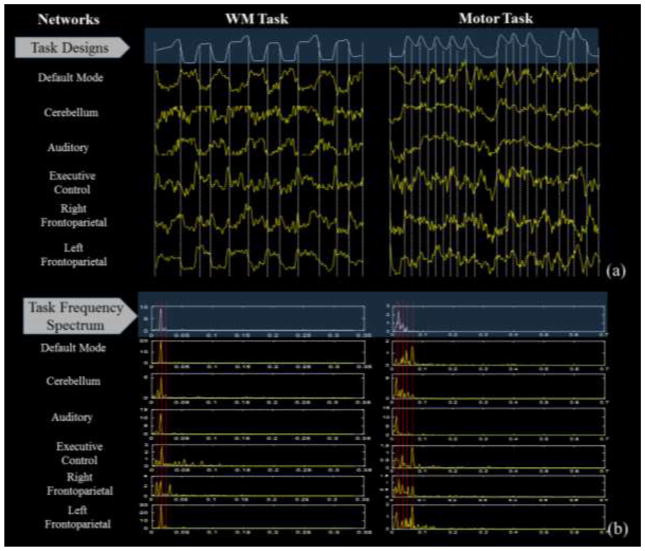
In addition, we explored the temporal and frequency features of the learned networks in Fig. 12. The temporal patterns corresponding to the networks in Fig. 11 are shown in Fig. 12. For each corresponding intrinsic network, we averaged the learned signal patterns from all the subjects in the same task (Fig. 12a), and at the same time we average the stimuli in each task as the global task curve (white curves on the top of Fig. 12a). And in Fig. 12b, the frequency spectrum of the task designs and network signals are visualized. From the inspection on the two task datasets, it’s evident that the temporal patterns of these networks are potentially tuned or affected by the task input, e.g., the temporal patterns of the default mode network tend to be like anti-task shape; the executive control network tends to peak at task change points, and more high frequency components could be observed as shown in Fig. 12b. These observations are in agreement with the functional mechanism of these networks (Smith et al., 2009). The frequency energy peaks of the networks in Fig. 12b are partially or fully in agreement with the task frequency spectrum. Additionally, quantitative correlation analysis can be found in Table. 9 and Supplemental Table. 2. From both tables, we can infer that DMN networks consistently exhibit anti-correlation with task design. The cerebellum and left frontoparietal networks exhibit high correlation with task designs.

Fig. 12.

(a) Comparison of temporal patterns of the spatially restricted networks with the task designs. (b) Comparison of frequency energy distribution with the task frequency spectrum.

Table 9.

The correlation of the temporal patterns in Fig. 12a with the task designs in Fig. 12a.

Correlation With Task Design	DMN	Cerebellum	Auditory	Executive Control	Right Frontoparietal	Left Frontoparietal
WM Task	−0.75	0.57	−0.59	0.27	0.25	0.82
Motor Task	−0.25	0.71	0.46	0.36	0.24	0.38

Note that we didn’t select network templates with conceptual conflict with our task design, like motor and visual networks, because motor networks should be learned with fixed task design in motor task data and visual networks are task-related networks in both data sets. On the other hand, from the temporal feature analysis in this section, we found that the activities of these well-established intrinsic networks are more or less coded by the task designs. So when modeling these networks with spatial restriction, we suggest to tune to a small value (like γ = 2×10⁻³) to avoid potential side effects. In addition, the spatial restriction could be set independently from the temporal constraint while training, so that it could be used for resting state fMRI analysis in the future.

3.6 Automatically Learned Concurrent Networks

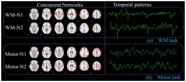
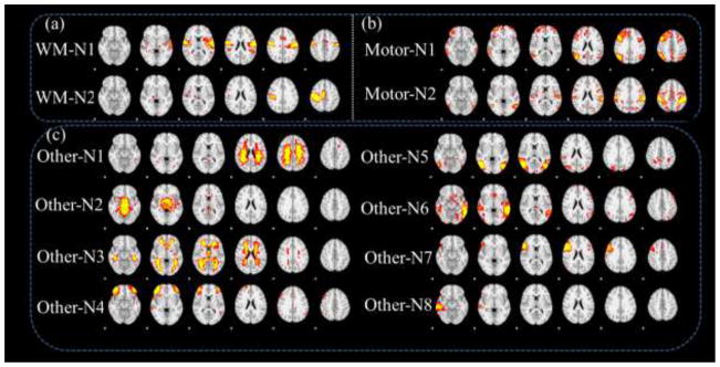
Besides the supervised networks in the previous two sections, multiple concurrent networks can also be learned from our method at the same time, as shown in Fig. 13. Although the temporal responses of these networks might not be directly interpreted in the second column of Fig. 13, it is quite interesting that some motor networks can be detected in the working memory task fMRI data, as shown in the spatial patterns of WM-N1 and WM-N2 in Fig. 13a. Meanwhile, some working memory networks can also be detected in the motor task data, as shown in the spatial patterns of Motor-N1 and Motor-N2 in Fig. 13b. This finding suggests that these brain networks intrinsically exist in the human brain, which might show different activity during different tasks. Additionally, through clustering all automatically learned networks from all subjects with spatial similarity as a metric, we found that the networks in Fig. 13 consistently exist across subjects, and their average patterns are shown in Fig. 14a and Fig. 14b. From the clustering analysis, we also found other concurrent networks (Fig. 14c) but cannot explain their spatial and temporal patterns. For instances, Other-N1 mainly concentrated in the white matter, while Other-N2 and Other-N3 located on the thalamus and ventricle areas, respectively. Other-N4 and Other-N5 are distributed bilaterally, while Other-N6, Other-N7 and Other-N8 are unilateral. It’s interesting that these networks could be consistently clustered from multiple subjects and different tasks, suggesting a common network architecture across different subjects and conditions. Meaningful interpretation of these networks entails further investigations in the future.

Fig. 13.

Automatically learned concurrent networks of one subject. Panel (a) is from the working memory task. Panel (b) is from the motor task. First Column: Spatial patterns of the learned networks. Column 2: Temporal patterns of the learned networks.

Fig. 14.

Averaged group-wise consistent networks through clustering. (a) The group-wise maps of networks in Fig. 13a. (b) The group-wise maps of networks in Fig. 13b. (c) Other group-wise networks from clustering method.

3.7 The Influence of Parameter Selection

Three parameters are crucial in our proposed method, i.e., λ, γ and the dictionary size. In this section, we investigated the influence of these parameters on the network reconstruction. In our experiments, we explored each parameter while the others are fixed.

Firstly, we set λ from 0 to 0.24 with interval of 0.04 (γ=2×10⁻³, dictionary size is set as 200). In supplemental Fig. 1, one task related network was visualized with different λ settings. From the figures, we could infer that, without the sparsity constraint, although we still have the network foci, the network looks quite noisy. If λ was set too high, the network foci are corrupted. So the parameter λ controls the network noise level and setting an appropriate λ could control the noise level of the networks. In this work, λ was chosen when the resultant networks showed comparable level of sparsity to GLM activations.

Secondly, we have introduced γ to control the intra-correlation of the learned dictionary. As we mentioned in Section 3.4, an appropriate γ could improve the estimation of the task networks. Actually, it’s also a tunable parameter, but not a very sensitive one. In our experiments, we set γ as 0 and from 2×10⁻⁵ to 2×10⁻¹ (λ =0.16, dictionary size is set as 200). The correlation matrices of the learned dictionaries are shown in Supplemental Fig. 2, and the maximum correlation values in the red block (constrained part) were shown in Supplemental Fig. 3. From both figures, we could see the correlation gradually decreased with increased γ. We also visualized one example task network by different settings of γ in Supplemental Fig. 4, from which we can see that with γ set as 0 and very small values, the foci of the network are not prominent. So we suggest to set γ> 2×10⁻⁴. However, as we mentioned in Section 3.5, high γ could cause side effects on the spatially constrained networks if the networks exhibit potential correlation with task design. With our experience, setting a moderate value, like γ= 2×10⁻³, could reach ideal balance.

Finally, with the optimal setting, λ =0.16 and γ= 2×10⁻³, we explored the influence of dictionary size. By setting dictionary size from 50 to 400, Supplemental Fig. 5 visualized examples of temporally constrained task network, spatially constrained DMN network and the automatically learned Motor-N1 network named in Section 3.6. Theoretically, the dictionary size can be over complete. However, in our experiment even with small dictionary size, the reconstructed networks are all meaningful and reliable. From supplemental Fig. 5, we could see that with the increment of dictionary size, the constrained task network and DMN network are quite stable and change only slightly. On the other hand, the automatically learned networks could be influenced by the dictionary size: the Motor-N1 network, which is consistent with dictionary size from 50 to 300, is decomposed into several sub-networks when dictionary size reaches 350 and 400. Currently, there is not criterion for an optimal dictionary size, because the mechanism and neuroscience meaning of the automatically learned networks remain elusive. We selected a moderate size of 200 for the current work and are in the process of developing new method to determine dictionary size.

In summary, parameter tuning could improve the performance of our method. Here, we recommend the optimal setting as dictionary size = 200, λ=0.16 and γ= 2×10⁻³, and the results in Section 3.2, Section 3.3, Section 3.5 and Section 3.6 are generated with these settings. In our experiments, we set the same parameter for two datasets with totally different acquisition protocols and the results are quite consistent and stable. Slightly tuning of parameters is suggested when the supervised SCC is applied on a new dataset. In the future works, we will explore solutions for automatic parameter setting.

4. DISCUSSION AND CONCLUSION

In this paper, we proposed a novel supervised dictionary learning and sparse coding method named supervised stochastic coordinate coding (SCC) for task fMRI data analysis. The major advantage of this method is that temporal models and spatial templates can be supervised as constraints for network inference, and at the same time, other concurrent networks can be learned automatically from data in a data-driven fashion. With the correspondence established by the supervised temporal and spatial information, group-wise statistics could be performed on both task-evoked and intrinsic networks. Furthermore, by group-wise clustering of the networks from automatic learning, other meaningful networks could be discovered.

We applied the proposed method on two independent fMRI data sets and obtained robust results. First, the task-evoked networks learned by our method are comparable with the GLM based activation at single subject level as well as at group level. Second, by utilizing motion parameters in the dictionary learning, motion artifacts would be removed while modeling brain networks, and by minimizing the intra-correlation, the task-evoked networks could be enhanced. Then, by restricting spatial templates, the major signal patterns of the well-known intrinsic networks could be learned and interpreted. In addition, the individual variability in spatial patterns could also be learned and evaluated. Finally, by clustering the spatial maps of the automatically learned networks, we also detected additional networks with high cross-subject consistency.

It should be noted that this work significantly improved the performance of the approach proposed in Lv et al., 2015a and Lv et al., 2015b. In the previous work with totally data-driven dictionary learning and sparse coding, the networks, especially task networks, are learned individualized and arbitrarily, e.g., one task network could be decomposed into multiple subnetworks or a few networks could be merged together. This makes it difficult to identify networks. Also these networks lack cross-subject correspondence, and as a result, the group-wise statistics could not be realized. The improvement of the supervised SCC lies in the following aspects. 1) The identification of task-evoked and intrinsic networks is realized and enhanced by supervised information. 2) With the correspondence established by supervised information, group-wise statistics could be performed. 3) The prior knowledge has been utilized in dictionary learning so that the hypothesize-driven and data-driven strategies are balanced. It should also be noted that the temporal constraint and spatial restriction could be applied independently while using the method. Therefore, the spatial restriction could be used for resting state fMRI analysis and network modeling, which will be explored in the future. We explored the influence of parameter selection of our method and suggested relatively optimal parameters. Future improvements and extensions of this work will be considered in the following perspectives. 1) The parameters such as the dictionary size, λ and γ are currently determined manually by trying different combinations, automatic or semi-automatic solutions for parameter selection will be explored in the future. 2) The networks learned by automatic learning and group-wise clustering could be potentially affected by the setting of dictionary size, and the interpretation and optimization of these networks entails further efforts. 3) This framework could be applied to other task/rest fMRI datasets, including applications to clinical fMRI data for discovery of network disruptions in brain disorders.

Highlights.

• Novel approach of sparse representation on the fMRI data.

• Temporal features and spatial patterns could be supervised in dictionary learning on fMRI data.

• Modeling brain networks with correspondence of prior knowledge makes group-wise analysis feasible.

• Automatic learning makes it flexible to detect meaningful concurrent brain networks hidden in the data.

References

- Andersson JL, Jenkinson M, Smith S. FMRIB Analysis Group of the University of Oxford. 2007. Non-linear registration, aka Spatial normalisation FMRIB technical report TR07JA2. [Google Scholar]
- Barch DM, Burgess GC, Harms MP, Petersen SE, Schlaggar BL, Corbetta M … WU-Minn HCP Consortium. Function in the human connectome: task-fMRI and individual differences in behavior. Neuroimage. 2013;80:169–189. doi: 10.1016/j.neuroimage.2013.05.033. [DOI] [PMC free article] [PubMed] [Google Scholar]
- Beckmann CF, Jenkinson M, Smith SM. General multilevel linear modeling for group analysis in FMRI. Neuroimage. 2003;20(2):1052–1063. doi: 10.1016/S1053-8119(03)00435-X. [DOI] [PubMed] [Google Scholar]
- Beck A, Teboulle M. A fast iterative shrinkage-thresholding algorithm for linear inverse problems. SIAM journal on imaging sciences. 2009;2(1):183–202. [Google Scholar]
- Bullmore E, Sporns O. Complex brain networks: graph theoretical analysis of structural and functional systems. Nature Reviews Neuroscience. 2009;10(3):186–198. doi: 10.1038/nrn2575. [DOI] [PubMed] [Google Scholar]
- Duncan J. The multiple-demand (MD) system of the primate brain: mental programs for intelligent behaviour. Trends in cognitive sciences. 2010;14(4):172–179. doi: 10.1016/j.tics.2010.01.004. [DOI] [PubMed] [Google Scholar]
- Efron B, Hastie T, Johnstone I, Tibshirani R. Least angle regression. The Annals of statistics. 2004;32(2):407–499. [Google Scholar]
- Faraco CC, Unsworth N, Langley J, Terry D, Li K, Zhang D, … Miller LS. Complex span tasks and hippocampal recruitment during working memory. NeuroImage. 2011;55(2):773–787. doi: 10.1016/j.neuroimage.2010.12.033. [DOI] [PubMed] [Google Scholar]
- Friston KJ, Holmes AP, Worsley KJ, Poline JP, Frith CD, Frackowiak RS. Statistical parametric maps in functional imaging: a general linear approach. Human brain mapping. 1994;2(4):189–210. [Google Scholar]
- Gazzaniga MS. The cognitive neurosciences. MIT press; 2004. [Google Scholar]
- Heeger DJ, Ress D. What does fMRI tell us about neuronal activity? Nature Reviews Neuroscience. 2002;3(2):142–151. doi: 10.1038/nrn730. [DOI] [PubMed] [Google Scholar]
- Jarrett K, Kavukcuoglu K, Ranzato MA, LeCun Y. What is the best multistage architecture for object recognition?. Computer Vision, 2009 IEEE 12th International Conference on; IEEE; 2009. Sep, pp. 2146–2153. [Google Scholar]
- Jenkinson M, Bannister P, Brady M, Smith S. Improved optimization for the robust and accurate linear registration and motion correction of brain images. Neuroimage. 2002;17(2):825–841. doi: 10.1016/s1053-8119(02)91132-8. [DOI] [PubMed] [Google Scholar]
- Kanwisher N. Functional specificity in the human brain: a window into the functional architecture of the mind. Proceedings of the National Academy of Sciences. 2010;107(25):11163–11170. doi: 10.1073/pnas.1005062107. [DOI] [PMC free article] [PubMed] [Google Scholar]
- Logothetis NK. What we can do and what we cannot do with fMRI. Nature. 2008;453(7197):869–878. doi: 10.1038/nature06976. [DOI] [PubMed] [Google Scholar]
- Lee K, Tak S, Ye JC. A data-driven sparse GLM for fMRI analysis using sparse dictionary learning with MDL criterion. Medical Imaging, IEEE Transactions on. 2011;30(5):1076–1089. doi: 10.1109/TMI.2010.2097275. [DOI] [PubMed] [Google Scholar]
- Lin B, Li Q, Sun Q, Lai MJ, Davidson I, Fan W, Ye J. Stochastic Coordinate Coding and Its Application for Drosophila Gene Expression Pattern Annotation. 2014 arXiv preprint arXiv:1407.8147.b. [Google Scholar]
- Lv J, Jiang X, Li X, Zhu D, Zhang S, Zhao S, … Liu T. Holistic Atlases of Functional Networks and Interactions Reveal Reciprocal Organizational Architecture of Cortical Function. Biomedical Engineering, IEEE Transactions on. 2015a;62(4):1120–1131. doi: 10.1109/TBME.2014.2369495. [DOI] [PubMed] [Google Scholar]
- Lv J, Jiang X, Li X, Zhu D, Chen H, Zhang T, … Liu T. Sparse representation of whole-brain FMRI signals for identification of functional networks. Medical image analysis. 2015b;20(1):112–134. doi: 10.1016/j.media.2014.10.011. [DOI] [PubMed] [Google Scholar]
- Lv J, Jiang X, Li X, Zhu D, Zhao S, Zhang T, … Liu T. Assessing effects of prenatal alcohol exposure using group-wise sparse representation of fMRI data. Psychiatry Research: Neuroimaging. 2015c;233(2):254–268. doi: 10.1016/j.pscychresns.2015.07.012. [DOI] [PMC free article] [PubMed] [Google Scholar]
- Mairal J, Bach F, Ponce J, Sapiro G. Online learning for matrix factorization and sparse coding. The Journal of Machine Learning Research. 2010;11:19–60. [Google Scholar]
- Olshausen BA. Emergence of simple-cell receptive field properties by learning a sparse code for natural images. Nature. 1996;381(6583):607–609. doi: 10.1038/381607a0. [DOI] [PubMed] [Google Scholar]
- Olshausen BA, Field DJ. Sparse coding of sensory inputs. Current opinion in neurobiology. 2004;14(4):481–487. doi: 10.1016/j.conb.2004.07.007. [DOI] [PubMed] [Google Scholar]
- Pessoa L. Beyond brain regions: Network perspective of cognition–emotion interactions. Behavioral and Brain Sciences. 2012;35(03):158–159. doi: 10.1017/S0140525X11001567. [DOI] [PubMed] [Google Scholar]
- Smith SM, Fox PT, Miller KL, Glahn DC, Fox PM, Mackay CE, … Beckmann CF. Correspondence of the brain’s functional architecture during activation and rest. Proceedings of the National Academy of Sciences. 2009;106(31):13040–13045. doi: 10.1073/pnas.0905267106. [DOI] [PMC free article] [PubMed] [Google Scholar]
- Tibshirani R. Regression shrinkage and selection via the lasso. Journal of the Royal Statistical Society. Series B (Methodological) 1996:267–288. [Google Scholar]
- Wright J, Yang AY, Ganesh A, Sastry SS, Ma Y. Robust face recognition via sparse representation. Pattern Analysis and Machine Intelligence, IEEE Transactions on. 2009;31(2):210–227. doi: 10.1109/TPAMI.2008.79. [DOI] [PubMed] [Google Scholar]
- Wu TT, Lange K. Coordinate descent algorithms for lasso penalized regression. The Annals of Applied Statistics. 2008:224–244. doi: 10.1214/10-AOAS388. [DOI] [PMC free article] [PubMed] [Google Scholar]
Associated Data
This section collects any data citations, data availability statements, or supplementary materials included in this article.