Smoothed Biasing Forces Yield Unbiased Free Energies with the Extended-System Adaptive Biasing Force Method

Abstract

We report a theoretical description and numerical tests of the extended-system adaptive biasing force method (eABF), together with an unbiased estimator of the free energy surface from eABF dynamics. Whereas the original ABF approach uses its running estimate of the free energy gradient as the adaptive biasing force, eABF is built on the idea that the exact free energy gradient is not necessary for efficient exploration, and that it is still possible to recover the exact free energy separately with an appropriate estimator. eABF does not directly bias the collective coordinates of interest, but rather fictitious variables that are harmonically coupled to them; therefore is does not require second derivative estimates, making it easily applicable to a wider range of problems than ABF. Furthermore, the extended variables present a smoother, coarse-grain-like sampling problem on a mollified free energy surface, leading to faster exploration and convergence. We also introduce CZAR, a simple, unbiased free energy estimator from eABF trajectories. eABF/CZAR converges to the physical free energy surface faster than standard ABF for a wide range of parameters.

Introduction

Coordinate-based free energy simulation methods accomplish two tasks: sample a reduced-dimension space of generalized coordinates, and estimate the associated free energy landscape. Among these, the adaptive biasing force method (ABF)¹⁻³ is an adaptive application of unconstrained thermodynamic integration (TI). In ABF, the running estimate of the free energy gradient from TI is used as the biasing force, hence combining the importance sampling and free energy estimation problems.

Here we investigate a combination of ABF with extended-system dynamics as in the Car–Parrinello metadynamics method.^4,5 This combination was introduced by Lelièvre et al.,^6,7 and is a part of the double-integration orthogonal space tempering method of Yang and co-workers, under the name Dynamic Reference Restraining.⁸ This extended-system ABF algorithm will henceforth be referred to as eABF. Instead of applying the ABF scheme to generalized variables that depend directly on atomic coordinates, eABF dynamics proceeds in a separate, explicit collective coordinate space with its own equations of motion, and these extended degrees of freedom are harmonically coupled to the collective variables in atomic coordinate space. As eABF does not rely on the free energy surface of interest for importance sampling, a separate estimator of the free energy is needed.

There are two possible benefits from the eABF approach. One is a gain in flexibility and efficiency due to separating the problems of sampling and free energy estimation, as has been investigated in recent studies.^9,10 We investigate and discuss this question in detail in this work. The second benefit is bypassing the stringent technical requirements for collective variables to be usable for ABF. The multidimensional TI formalism¹¹ used by our implementation of ABF¹² entails some practical limitations: collective variables are required to be mutually orthogonal, and orthogonal to constraints; furthermore, a Jacobian term, which depends on second derivatives of the coordinates, must be calculated. While defining an effective, low-dimension collective coordinate space for molecular processes is often daunting to begin with, additional restrictions on the coordinates that can be used for ABF reduce the applicability of the method in the most challenging cases. eABF relaxes these requirements, making the method applicable to any set of variables whose individual values and gradients can be readily computed.

Below, we present the principles of eABF dynamics in one and multiple dimensions, as well its combination with standard ABF in what we term “semi-eABF”. We derive some properties of eABF-biased distributions of the coordinates, which are useful for understanding the sampling efficiency of the method. We then describe numerical tests and explain the effects of its parameters on convergence, most notably the strength of coupling between the geometric coordinate and the fictitious variable. We investigate the role of noise reduction through mollification of the measured forces by fluctuations of the coupling spring. We introduce the corrected z-averaged restraint (CZAR) estimator of the “true” free energy based on eABF trajectories. Finally, we test the convergence and accuracy of eABF/CZAR and compare it to ABF as well as an Umbrella-Integration-based estimator.

Theory

Theory of eABF

Standard ABF

Let us recall the principles and notations of the ABF method,¹ the direct parent of eABF. Consider a set of particles of coordinates , subject to constraints of the form σ_k(q) = 0, and whose physical distribution is the canonical ensemble associated with the potential V(q) at temperature T. Within that ensemble, we wish to sample a vector generalized coordinate (collective variable) of physical interest, z = ξ(q). ABF is an adaptively biased dynamics that produces, in the long-time limit, a uniform distribution of ξ.^1,3,7 ABF also yields an unbiased estimate of the free energy profile (or potential of mean force, PMF) A(z), which is defined by

1

where ρ is the equilibrium probability distribution of ξ. The time-dependent biasing force in ABF is the running estimate of the free energy gradient.

Our implementation of ABF¹² relies on multidimensional thermodynamic integration as expressed by Ciccotti et al.¹¹ For each coordinate ξ_i, let v_i be any vector field on atomic coordinates (, where N is the number of atoms) satisfying, for all j and k,

2

3

We call v_i the inverse gradient of ξ_i.¹² A possible choice is v_i = ∑_jG_i,j^–1 ∇ξ_i, provided that the matrix G ≡ (∇ξ_i·∇ξ_j)_i,j is invertible.⁶ This, however, is not often practical: in simpler cases intuition is sufficient to exhibit valid choices of v, whereas in more complex cases, obtaining v in closed form from this expression is difficult, if at all possible.

The ith partial derivative of the free energy surface A may then be calculated as the ξ-conditioned ensemble average of the instantaneous collective force F_i^ξ:¹¹

4

Depending on the function ξ, calculation of the divergence ∇·v_i, which typically implies second derivatives of ξ_i, may be onerous or impossible to express in closed form. It then becomes desirable to replace ABF dynamics on coordinate ξ with a dynamics that approximates it at a lower cost (including the cost of developing algorithms and production-quality code).

eABF consists in performing ABF dynamics on a fictitious coordinate that fluctuates around ξ(q). We shall now present eABF in detail, first on a scalar variable ξ for simplicity, then in higher dimension.

eABF on a scalar variable

In eABF, we consider the extended system (q, λ), where λ is a fictitious, nonphysical degree of freedom with mass m_λ. λ evolves in time according to Langevin dynamics at the same temperature as the rest of the system. To ensure that λ approximates ξ, we couple these quantities with the harmonic potential (k/2) (ξ(q) – λ)². eABF can therefore be seen as a multiscale simulation method, where λ_t represents a coarse-grained dynamics coupled to the atomic dynamics (Figure 1). We then define eABF on coordinate ξ as standard ABF dynamics on the extended coordinate ξ^ext, where ξ^ext (q, λ) ≡ λ.

Figure 1.

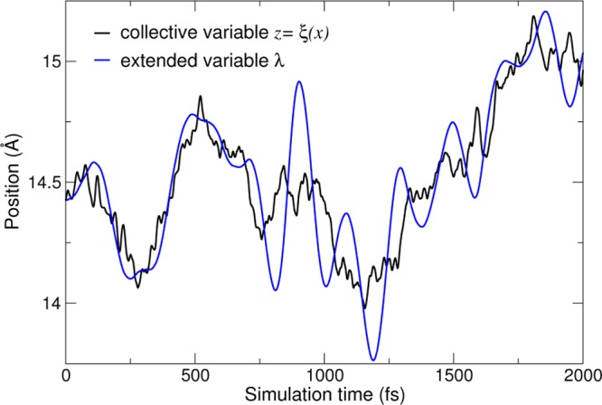
Time trajectories of the collective variable ξ(x_t) (black) and the fictitious coordinate λ_t (blue) for the deca-alanine system (see Computational Details for details).

The obvious choice of inverse gradient v is equal to the gradient ∇ξ^ext, that is, a vector with null components for all q, and 1 for λ. This satisfies eq 2 and eq 3 because v has no support on coordinates q involved in constraints. The instantaneous force of eq 4 then reduces to the harmonic force from the coupling potential, which can be calculated regardless of the geometry of ξ, and without using the physical forces −∇V(q), in contrast to standard ABF.

The main convergence property of ABF applies, that is, the biased dynamics of λ is less metastable than the unbiased one, and its limiting probability distribution is uniform, yielding a form of “optimal” sampling. The key intuition behind eABF is that efficient sampling of λ will result in efficient sampling of ξ, given sufficient coupling between those two variables. We will show numerically that this is verified, and examine the requirement on the coupling strength.

In the absence of adaptive bias, the extended potential is

5

and the equilibrium marginal distribution of λ depends on k:

6

The corresponding PMF in λ is defined by

7

In the following, probability distributions are expressed up to a normalization constant, and free energy profiles up to an implicit additive constant, without loss of precision or generality.

The integral in (6) may be recast by inserting ∫δ(ξ(q) – z) dz = 1:

8

That is, the marginal distribution of the extended variable λ is that of ξ(q) convolved with a Gaussian kernel of variance σ² ≡ (βk)⁻¹. Therefore, in the tight-coupling limit (large k, small σ), ρ^k becomes arbitrarily close to ρ, and the extended PMF A^k, to the physical PMF A. A numerical example comparing these two quantities (Figure 2) illustrates A^k as a smoothed or mollified version of A.

Figure 2.

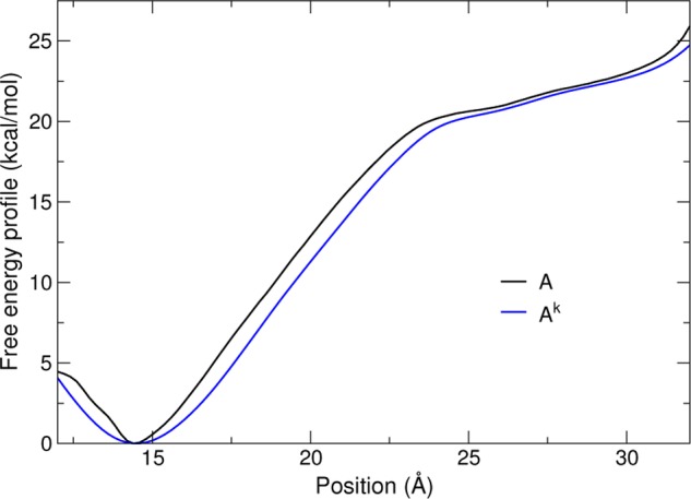
Comparison of the physical free energy profile A(z) (black) and that of the extended variable, A^k(λ) (blue) for the deca-alanine system with loose coupling (σ = 0.5 Å).

Under eABF dynamics, the applied bias on λ is the running estimate of the average spring force:

9

where the angle brackets indicate a canonical average conditioned by λ = λ*. The system is driven by a time-dependent biased potential Ṽ_t(q, λ) that converges toward

10

which generates the following biased Boltzmann distribution:

11

Integrating over q and inserting eq 6 shows that this results in a uniform marginal distribution of λ, ρ̃^k(λ) = constant, which is the ABF result for the extended variable λ.

Integrating eq 11 over the conditional measure δ_ξ(q)–z yields the joint distribution of (z, λ):

12

Integrating over λ gives the biased marginal in z:

13

where we have substituted A^k with its definition (eq 7). Finally, substituting eq 8 into eq 13, we obtain an explicit relationship between the unbiased and biased z-distributions:

14

which can be summarized as

15

where G_σ stands for the Gaussian kernel of variance σ², and * for convolution. In the high-k, low-σ limit, convolution by the kernel becomes the identity operator, and the correction factor becomes ρ(z)⁻¹. Thus, the biased limiting distribution ρ̃(z) becomes uniform, and eABF in the high-k limit recovers the behavior of standard ABF on coordinate z = ξ(q).

Vector eABF

The approach outlined above may be extended to higher-dimension variables, following the principles of multidimensional ABF.¹² Given a d-dimensional vector collective variable ξ(q) = (ξ_i(q))_i, we augment the system with a vector of d extended variables λ = (λ_i)_i, coupled through as many harmonic potentials (1/2) k_i (ξ(q) – λ_i)². Because the components ξ_i may have different physical dimensions, the spring constants k_i are not generally commensurable.

To recover the multidimensional thermodynamic integration formalism recalled above, we define the inverse gradient vector v_i as equal to the gradient ∇_(q, λ) ξ_i^ext, that is, the vector with component 1 on coordinate λ_i and zero elsewhere. This satisfies the conditions of eqs 2 and 3. Components of the adaptive biasing force are then

16

where the angle brackets indicate an average with respect to the canonical distribution of (q, λ) conditioned by λ = λ*. The case of a two-dimensional coordinate is illustrated in numerical tests below.

Semi-eABF

Consider the special case of two collective variables ξ₁ and ξ₂. One may then run a semi-eABF simulation, that is, a simulation in extended space (q, λ) with a harmonic potential coupling λ and ξ₂(q), and an ABF bias on the two-dimensional coordinate ξ^ext(q, λ) ≡ (ξ₁(q), λ).

A vector field v₁ needs to be defined, verifying v₁(q) ·∇ξ₁(q) = 1 for all q (eq 2), and orthogonal to constraints (eq 3). The mutual orthogonality condition of eq 2 is trivially fulfilled because the second coordinate is independent of q. The biasing forces may then be calculated based on

17

18

where the angle brackets indicate averages with respect to the canonical distribution of (q, λ) conditioned by (ξ₁(q) = z₁, λ = λ*).

More generally, one may run ABF dynamics on a vector variable involving any combination of geometric coordinates and fictitious variables. Numerical tests of the semi-eABF approach in two dimensions are presented below, together with an appropriate free-energy estimator.

Estimators of the Original Free Energy Gradient

The eABF free energy gradient estimator converges in the long-time limit to A^k ′(λ), which is not the “true”, physical free energy gradient A′(z). Here we discuss how to estimate the physical free energy gradient from an eABF simulation.

Naive Estimator

The simplest estimator uses A^k as an approximation to the physical PMF, A(z). This, however, is not asymptotically unbiased in the long-time limit, because of the convolution in eq 8, as can be seen in Figure 2. A^k does converge to A only in the high-k limit. Below, we describe and test two other estimators, one of which is asymptotically unbiased regardless of k. Another option, since A^k is related to A by convolution, is to apply a generic deconvolution algorithm;¹³ however, that approach again yields a biased estimator.

Zheng and Yang Estimator

Zheng and Yang proposed a free energy estimator in the context of the orthogonal space tempering method,⁸ but it is applicable more generally to any eABF-like simulation. Considering that each λ-value is a state wherein z is sampled under a harmonic restraint, the free energy derivative can be written based on umbrella integration.¹⁴ The final estimate of the free energy derivative is a weighted average of the umbrella integration values from different “restraining ensembles” (λ-states):⁸

19

where ρ̃ (z|λ) is the observed, bias distribution of ξ(q) conditioned by λ. Umbrella integration further assumes that this distribution is nearly Gaussian, hence its log-derivative may be approximated based on its mean ⟨z ⟩_λ and variance (σ_λ^z)²:

20

This assumption reduces the variance of the estimator, but introduces a bias that formally vanishes only in the high-k regime, when ρ(z|λ) becomes peaked and tends toward a Gaussian.

In the past years, we informally provided the community with an implementation of the Zheng/Yang estimator as a post-treatment of eABF trajectories, which was inefficient for large amounts of data. This was improved by an on-the-fly implementation that was published recently.¹⁵

Corrected z-averaged restraint (CZAR)

We propose here an asymptotically unbiased estimator of A, named corrected z-averaged restraint (CZAR). Below, we introduce this estimator based on physical intuition (see Supporting Information for a formal derivation).

Consider the eABF-biased dynamics of coordinate z = ξ(q). This coordinate only feels the eABF bias through the spring force k(λ – z). Thus, at a given value of z, the biasing force on coordinate λ results in an effective average biasing force on z equal to k(⟨λ⟩_z – z) (where ⟨λ⟩_z is the conditional average of λ at a given value of z). The free energy gradient is the log-derivative of the unbiased distribution ρ:

21

from which we can derive a relationship with the eABF-biased distribution ρ̃:

22

The right-hand side can be estimated numerically from the time trajectory of (z, λ).

We note that eq 22 is related to eq 19 by swapping the integration with respect to λ and differentiation with respect to z. Thus, the main difference between the CZAR and Zheng/Yang approaches is that the latter relies on a Gaussian approximation for the conditional distributions of z. A practical benefit of CZAR is that it does not require defining discrete λ-states, which makes implementation simpler and removes a tunable parameter.

Multidimensional CZAR

The CZAR estimator generalizes to eABF on a vector variable of arbitrary dimension, z = (z_i)_i = (ξ_i(q))_i. Each component of the free energy gradient may be estimated as

23

The derivation is provided in the Supporting Information, in dimension 2 for the sake of simplicity. It extends to arbitrary dimension in a straightforward way.

The CZAR estimator is valid for standard ABF as well, if the z-averaged force is replaced with the average force of ABF for “non-extended” coordinates. The log-derivative of the ABF-biased distribution vanishes for long times as the distribution becomes uniform. Thus, CZAR may be used transparently in the semi-eABF case, as it provides unbiased estimates of the free energy gradient along both extended and nonextended variables. This is used in the numerical tests of semi-eABF below.

Implementation

Implementation of eABF Dynamics

Our eABF implementation in the Collective Variables Module (Colvars)¹⁶ is essentially a combination of two pre-existing features: extended-system coordinates, and multidimensional ABF.¹² The extended Lagrangian functionality of the colvars module includes separate velocity-Verlet or Langevin integrators, independent from that of the underlying MD engine, as well as harmonic restraints coupling each extended degree of freedom to its counterpart collective variable.

Activating extended dynamics introduces two tunable parameters for each extended coordinate: integrating the Langevin equation of motion requires that the coordinate be assigned a fictitious mass, and the harmonic spring is defined by an arbitrary force constant. Rather than choosing those parameters directly, the Colvars implementation relies on an equivalent pair of quantities whose choice is more intuitive: the “thermal width” of the coupling, σ, which is also the standard deviation of the Gaussian kernel in eq 8, and its time constant τ (the period of the oscillator). They are determined from the following expressions:

24

25

where m is the fictitious mass and k is the harmonic force constant. Broadly speaking, if λ is to approximate ξ(q), then a small value of the tolerance σ is desirable. Conversely, the oscillator period should be much larger than the MD time step for stability of the integrator. More refined criteria for choosing these parameters will emerge from the numerical tests described below.

One practical benefit of implementing eABF over standard ABF, besides doing away with geometric complexity, is estimating the free energy gradient without needing the values of atomic forces. In large-scale parallel applications where NAMD¹⁷ and LAMMPS¹⁸ are often used, this removes the need to gather these atomic forces on the computing node tasked with executing the ABF algorithm. The decrease in interprocess communications should yield scaling improvements when many particles are involved in the definition of the collective variable.

Implementation of the CZAR Free Energy Estimator

We provide an implementation of the new CZAR estimator within the Colvars Module.¹⁶ It is de facto available for any combination of MD engine and platform supported by the Colvars, most notably, NAMD¹⁷ and LAMMPS.¹⁸ The algorithm is lightweight and relies on two accumulators that are updated at every time step: the z-conditioned average forces k⟨z_k – λ⟩_z, and the biased z marginal distribution, ρ̃(z). These two quantities are only combined at output time, to yield the free energy gradient estimate according to eq 22. The implementation, as with most Colvars functionality, supports an arbitrary number of variables. In one-dimensional cases, the gradient is integrated automatically using the trapezoidal rule. In multidimensional cases, the gradient must be integrated in a postprocessing step to yield the free energy surface. To this end, we use our discrete Markov chain Monte Carlo algorithm¹² in this work for practical reasons, but in principle any Poisson solver with adequate boundary conditions could be used.¹⁹

Computational Details

The test systems considered here were two small peptides in vacuum that were used in many studies before. The helical peptide deca-alanine was associated with its end-to-end distance (using the first and last α carbon atoms, in the absence of bond constraints). For two-dimensional tests, conformation of the dipeptide mimic N-acetyl-N-methyl-l-alanylamide (NANMA) was described by its central Ramachandran angles φ and ψ.

Simulations were run with the development version of NAMD 2.12,¹⁷ together with the Collective Variables Module¹⁶ version 2016-09-03, which will be included in NAMD 2.12. In vacuo systems were modeled by the CHARMM22 force field, and simulated with a time step of 0.5 fs with Langevin dynamics at 300 K and a damping coefficient of 5 ps^–1. The Zheng and Yang umbrella integration estimator^8,14 was used in its NAMD/Colvars implementation by Fu et al.¹⁵

Convergence of free energy gradient estimators was assessed as follows. For each set of parameters, 10 simulations were started using different random seeds and stochastic initial velocities, and run for 10 ns each. For assessing the convergence of true free energy estimators, sampling was increased to 20 simulations of 20 ns each to account for their higher variance. Values of the estimators to be tested were saved every nanosecond. The average of the final estimates of the free energy gradient from those replicas was the target for measuring “relative” convergence toward the limiting value of a given estimator under a given set of parameters. Reference ABF simulations were run under the same conditions except for the extended variables. The average ABF gradient from those reference simulations was the target to test for “absolute” convergence toward the true free energy gradient. For each individual test simulation, the root-mean-square distance from the estimated gradient to the target was calculated as a function of sampling time. The average and standard deviations of these distances over sets of simulations were used for comparing the accuracy and rate of convergence of estimators, and are plotted in Figures in the Results section.

Results and Discussion

Convergence of eABF

When estimating the free energy profile A(z) in an eABF simulation, convergence occurs at two levels. At the level of eABF itself, the free energy gradient estimator converges toward A^k′(λ), and the observed distribution of λ becomes uniform. This depends on tunable eABF parameters σ and τ, and on the delay parameter fullSamples. The second level is convergence of the estimators of A(z) based on the eABF trajectory (z_t, λ_t). The latter depends on the choice of estimator, and in the case of the Zheng/Yang and CZAR estimators described above, on good sampling of the joint distribution of z and λ.

Because the methods are intended for large-scale molecular simulations where sampling time is necessarily limited, we test the estimators and parameter sets based on their rate of convergence at short and moderate times (10 ns for the fast deca-alanine system).

The fullSamples parameter controls when enough sampling has been collected in one given bin for the adaptive biasing force to be introduced. To ensure continuity of the force as a function of time, the force is scaled by a linear ramp that goes from zero to one as the local sample count evolves between half the value of fullSamples and its full value.¹² The top panel in Figure 3 shows convergence rates of test simulations as a function of fullSamples. While the deviation at the end of the 10 ns simulations is equivalent, it can be seen to affect the initial convergence rate. A value of zero leads to transient overcompensation of the underlying free-energy, with strong dispersion of the results in the initial 4 ns for this particular case. This relaxation time could be much longer for more slowly relaxing systems, however, which is why larger values are advisable. Even for this toy system, a value of 2000 samples gives the fastest short-time convergence, as well as nearly optimal accuracy in the intermediate regime (4–8 ns) until the accuracies of all simulation sets converge at 10 ns. The fullSamples parameter is not specific of eABF, yet its role is not necessarily identical in eABF as in standard ABF. Tests of ABF on the same system showed that a value of 0 for fullSamples did not impair convergence.²⁰ This confirms that short-time scale relaxation properties of ABF and eABF are substantially different, as eABF dynamics is dominated by the relatively slow oscillations of the fictitious degree of freedom (Figures 1 and 4). On longer time scales, however, the limiting factor becomes orthogonal relaxation of slow degrees of freedom that are not captured by the chosen transition coordinate. That slow phenomenon occurs under similar circumstances in ABF and eABF. It is not well-captured by a small gas-phase system such as this one, yet slower systems would not lend themselves to precise statistical characterization.

Figure 3.

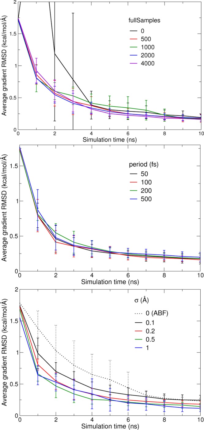
Convergence rate of eABF simulations as a function of the fullSamples parameter (upper panel), coupling time scale τ defined in eq 25 (middle panel), and coupling width σ defined in eq 24 (lower panel). The graphs show the RMS deviation of the eABF free energy gradient from an estimate of its limiting value, as a function of sampling time, averaged over ten 10-ns trajectories (error bars indicate standard deviation over the 10-fold average). Dotted line is from standard (non-extended-system) ABF simulations.

Figure 4.

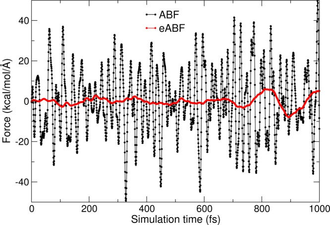
Time trajectories of the spring force in eABF (red) and the instantaneous collective force in ABF (black) for the deca-alanine system with σ = 0.2 Å. Data points are shown for every MD time step, here, every 0.5 fs.

Like fullSamples, the fluctuation period τ of the oscillator (defined in Equation 25) has no measurable influence on the deviation after 10 ns of simulation (Figure 3, middle). However, it does slightly influence the rate of convergence for shorter times. For this system, we find 100 fs to give the fastest convergence. A shorter time of 50 fs gives similarly fast convergence, yet this is only possible because we use a short MD integration time step of 0.5 fs in these gas-phase simulations. For condensed-phase simulations with longer timesteps, larger values of τ may be required to guarantee the accuracy of the extended-system trajectory: we recommend scaling it with the integration time step of the extended variable. Unless otherwise stated, other eABF simulations of the deca-alanine system are performed with fullSamples set to 2000 and a τ of 100 fs.

The key parameter of an eABF simulation is the coupling width σ, whose effect on convergence is illustrated by the lower panel of Figure 3. In the σ →0 limit, eABF is equivalent to standard ABF. The initial rate of convergence is simply an increasing function of σ: broader fluctuations of the fictitious degree of freedom appear to accelerate convergence. The slowest initial rate is obtained for standard ABF. This order is still valid at the end of the 10 ns interval, although error values have come closer together. Standard ABF and eABF at σ = 0.1 still have the highest variance. This result is surprising in the sense that higher values of σ make the simulation more “approximate” or “blurry”. However, this expected loss of accuracy leads to a gain in precision.

In ABF, fluctuations of the instantaneous force F_ξ are dominated by high-frequency terms due to bonded interactions (Figure 4). In eABF, the mean square fluctuation of the spring force σ_F² is of the order of k/β, which implies:

26

Thus, the choice of σ is a trade-off between fluctuations of the extended variable (bias of A^k as an estimator of A) and fluctuations of the extended force (variance of A^k): a high σ, low k will yield a limiting value of A^k that is very different from A but is estimated with low variance. However, the bias on A^k can be corrected by the estimators described below, which displaces the optimal compromise toward a soft (low k) rather than a stiff spring (high k). As evidenced numerically in Figure 4, even a moderately soft spring results in considerable noise reduction with respect to ABF.

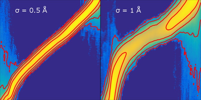
The upper panel of Figure 5 shows the joint biased distribution ρ̃(z, λ) observed for four different values of σ. These distributions observed numerically agree well with the prediction of eq 12 based on numerical estimates of A and A^k (data not shown). The common feature is that the marginal distribution in λ is nearly uniform, thanks to the eABF bias. Setting σ = 0.1 Å enforces near equality of the two variables, leading to a very narrow joint distribution and a nearly uniform z-marginal as well (lower panel of Figure 5). For looser coupling, the distribution broadens. At σ = 0.5, the high-probability region deviates visibly from the equality line, leading to undersampling of low values of z. At σ = 1, sampling along z becomes strongly nonuniform, with variations across 3 orders of magnitude. In this example, eABF sampling is most effective for σ between 0.2 and 0.5 Å, that is, where the mollification is significant but not sufficient to impede sampling along z.

Figure 5.

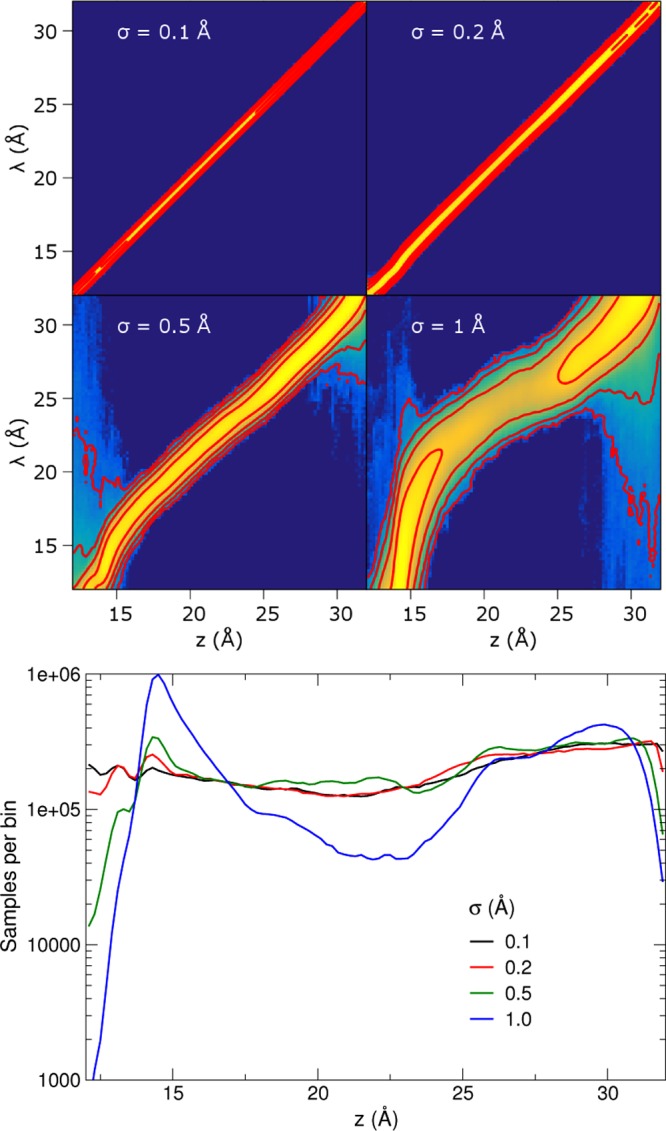
Upper: Observed joint distribution of (z, λ), the physical and extended coordinates, in eABF sampling of the deca-alanine system, for different values of σ. The scale is logarithmic, with red isovalue lines separated by a factor of 10 in probability density. Lower: Observed marginal distribution of z = ξ(q) from eABF sampling at different values of the coupling width σ for the deca-alanine system, plotted on a logarithmic scale.

Therefore, the drawback of a softer spring does not directly reside in the greater difference between A and A^k, but rather in the greater deviation of the limiting biased distribution of z from uniformity, eventually yielding poor sampling as high-free-energy regions in z may be missed despite complete sampling over λ.

Since the eABF bias differs from the optimal bias by Gaussian convolution (eq 13), deviations of ρ̃(z) from uniformity are related to the difference between ρ and its convolution. Considering the convolved of ρ by a Gaussian of variance σ² as an approximation to ρ(z) in the small-σ limit, it can be shown (see Supporting Information) that the error is bounded by ∥ρ″∥_L^∞σ²/2. That is, deviation from uniform sampling depends on the curvature of ρ(z). One may see from Figure 5 that sampling of z is reduced in concave regions of the PMF (hence of ρ) and increased in convex regions. As a result, the optimal value of σ for a given application depends on the curvature of ρ.

Convergence of Free Energy Estimators

Figure 6 shows the convergence toward the “true” free energy derivative A′(z) of the naive, Zheng/Yang (ZY), and CZAR estimators compared to standard ABF for different values of σ. The long-time bias of the naive estimator is clearly apparent for larger values of σ, but this estimator still proves faster-converging than standard ABF, and as accurate at t = 20 ns, for σ equal to 0.1 Å.

Figure 6.

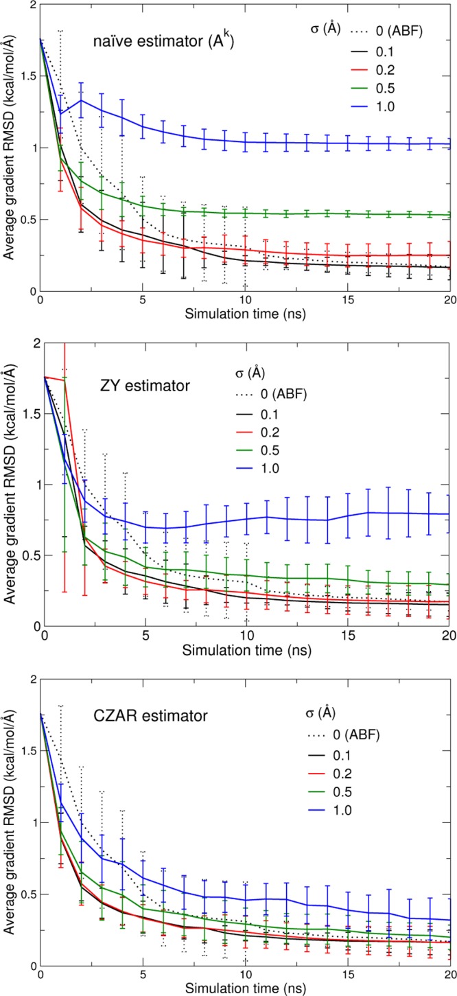
Convergence of the naive (top), Zheng/Yang (middle), and CZAR (bottom) free energy estimators, as a function of the coupling parameter σ. The graphs show the RMS deviation from the converged, true free energy gradient of each free energy gradient estimator as a function of sampling time, averaged over 20 20 ns trajectories (error bars indicate standard deviation over the 20-fold average). The dotted line is from a set of standard (nonextended system) ABF simulations.

On this time scale, the asymptotic bias of the ZY estimator at finite σ is only visible for σ of 0.5 or 1 Å: on those conditions, the Gaussian assumption (20) for the conditional distribution is not verified. For lower values of σ, the bias is masked by the error due to variance: the mean error at 20 ns is equivalent to that of CZAR or standard ABF. Still, the convergence rate is slightly slower at 0.2 Å and at 0.1 Å, with a greater dispersion. Since the CZAR and ZY estimators share their mean force term, this could be ascribed to noise in the two-dimensional (z, λ) histogram, which the Gaussian approximation may not erase at short times in less-populated regions of the histogram. Another contributing factor could be the error due to discretization along λ.

The defining feature of CZAR is its robustness with respect to σ, directly deriving from its asymptotically unbiased nature. Its rate of convergence, however, depends on efficient sampling along z. For too large values of σ (here, 1 Å), enhanced sampling along λ leaves some metastability or unsampled regions along ξ (Figure 5), leading to slower convergence of the PMF estimator (blue line).

In constrast with convergence of the mollified eABF free energy (Figure 3), all estimators seem more accurate at small σ (0.1 Å), but the CZAR estimator shows much more robustness with respect to σ.

Two-Dimensional Case

On the two-dimensional coordinate describing the NANMA peptide, the PMF estimates from eABF/CZAR and standard ABF are visually indistinguishable after 100 ns of sampling (Figure 7). A more quantitative view of the convergence is given by the upper panel of Figure 8. The optimal value of σ here is 5°. σ = 1° produces a high initial error, certainly due to the high variance of the 2D (φ, ψ) histogram at short sampling times. At 100 ns, this estimate has reached the error of standard ABF. Conversely, the σ = 10° simulation shows a high initial convergence rate, but at later times, its convergence is impeded by poor sampling along (φ, ψ) due to insufficient coupling to (λ_φ, λ_ψ), similar to the σ = 1 Å case for deca-alanine (Figure 5).

Figure 7.

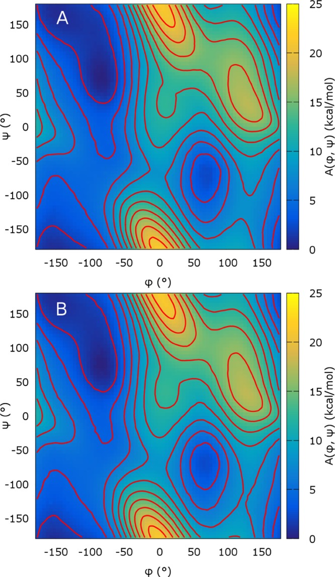
Two-dimensional free energy surface for the Ramachandran angles of NANMA in vacuum, reconstructed by standard ABF (A) and eABF with the CZAR estimator (B). Red isovalue lines are separated by 2 kcal/mol. Each simulation is 100 ns long.

Figure 8.

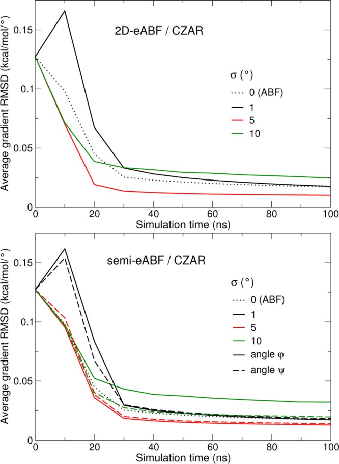
Convergence of the eABF/CZAR estimator of the two-dimensional free-energy gradients of NANMA, for a 2D eABF dynamics (upper panel) and semi-eABF dynamics (lower panel) with an extended coordinate coupled to either angle φ or ψ. Data is provided for three values of σ. Convergence of standard 2D ABF is shown for reference (dotted line).

The semi-eABF case is a form of 2D-ABF dynamics where one of the variables is biased directly, while the other is coupled to a fictitious degree of freedom that is biased. The results are largely similar to the 2D-eABF case, demonstrating the practical effectiveness of the approach. There is one interesting exception: the loose coupling case (σ = 10°), which shows slower convergence in 2D: eABF converges well when only the angle ψ is treated with an extended variable. This results from the anisotropic shape of the 2D PMF, where the barriers are more pronounced along φ than along ψ (Figure 7).

Conclusion

The eABF approach is a generalization of ABF, when applied to fictitious degrees of freedom coupled to generalized coordinates of interest. In contrast to ABF, it imposes no requirements as to what combinations of coordinates may be used, and only their gradients, not their second derivatives, are needed. eABF sampling is more effective than ABF due to the noise reduction effect of the fluctuations of the extended variable, as well as the nonlocal effect of the biasing force. We introduce CZAR, a conceptually simple, asymptotically unbiased estimator of the free energy that converges faster than ABF for a broad range of coupling strengths.

Thus, we have shown that the deviation of A^k from A is not damaging, as long as sampling of the actual geometric coordinate is efficacious. This stems from the essential difference between eABF and ABF, that is, separating the force used for sampling from the free energy gradient estimator. In ABF, the free energy that is being estimated is used exactly to accelerate the dynamics. eABF decouples the sampling bias and free energy estimate, leaving some flexibility to use a biased estimator with reduced variance and fast convergence for sampling, while still ultimately benefiting from an unbiased free energy estimator. In this sense, eABF is similar in spirit to a recently proposed approach, combining metadynamics for exploration and a separate free energy estimator.¹⁰ Indeed, the convergence rate of eABF/CZAR as a free energy estimator compares favorably to that of standard ABF, essentially because it combines efficient exploration on a smoothed free energy surface with an unbiased estimator of the actual free energy.

eABF is applicable where ABF is not, in particular for elaborate generalized coordinates where calculation of second derivatives is cumbersome, and for sets of coordinates where orthogonality of the inverse gradient (eq 2) is difficult to satisfy. Its added algorithmic complexity (integrator for the extended equations of motion and free energy estimator) is offset by the reduced geometric calculations. There are two additional tunable parameters in eABF. However, we have shown that one of them, the oscillation time, has limited impact on convergence, and the other, the coupling width, has a range of safe values, particularly if a robust, asymptotically unbiased free energy estimator is used.

Based on these results, it may be argued that eABF/CZAR is always preferable to ABF for its rate of convergence, regardless of practical implementation considerations. This may become clearer when several large-scale, numerically challenging applications are documented.

Supporting Information Available

The Supporting Information is available free of charge on the ACS Publications website at DOI: 10.1021/acs.jpcb.6b10055.

• Derivation of formulas used in the text (PDF)

The authors declare no competing financial interest.

References

- Darve E.; Pohorille A. Calculating free energies using average force. J. Chem. Phys. 2001, 115, 9169–9183. 10.1063/1.1410978. [DOI] [Google Scholar]
- Darve E.; Rodríguez-Gómez D.; Pohorille A. Adaptive biasing force method for scalar and vector free energy calculations. J. Chem. Phys. 2008, 128, 144120. 10.1063/1.2829861. [DOI] [PubMed] [Google Scholar]
- Comer J.; Gumbart J. C.; Hénin J.; Lelièvre T.; Pohorille A.; Chipot C. The adaptive biasing force method: everything you always wanted to know but were afraid to ask. J. Phys. Chem. B 2015, 119, 1129–1151. 10.1021/jp506633n. [DOI] [PMC free article] [PubMed] [Google Scholar]
- Car R.; Parrinello M. Unified approach for molecular dynamics and density-functional theory. Phys. Rev. Lett. 1985, 55, 2471–2474. 10.1103/PhysRevLett.55.2471. [DOI] [PubMed] [Google Scholar]
- Iannuzzi M.; Laio A.; Parrinello M. Efficient exploration of reactive potential energy surfaces using Car-Parrinello molecular dynamics. Phys. Rev. Lett. 2003, 90, 238302. 10.1103/PhysRevLett.90.238302. [DOI] [PubMed] [Google Scholar]
- Lelièvre T.; Rousset M.; Stoltz G. Computation of free energy profiles with parallel adaptive dynamics. J. Chem. Phys. 2007, 126, 134111. 10.1063/1.2711185. [DOI] [PubMed] [Google Scholar]
- Lelièvre T.; Rousset M.; Stoltz G.. Free Energy Computations: A Mathematical Perspective; Imperial College Press: London, 2010. [Google Scholar]
- Zheng L.; Yang W. Practically efficient and robust free energy calculations: Double-integration orthogonal space tempering. J. Chem. Theory Comput. 2012, 8, 810–823. 10.1021/ct200726v. [DOI] [PubMed] [Google Scholar]
- Cao L.; Stoltz G.; Lelièvre T.; Marinica M.-C.; Athènes M. Free energy calculations from adaptive molecular dynamics simulations with adiabatic reweighting. J. Chem. Phys. 2014, 140, 104108. 10.1063/1.4866811. [DOI] [PubMed] [Google Scholar]
- Mones L.; Bernstein N.; Csányi G. Exploration, sampling and reconstruction of free energy surfaces with Gaussian process regression. J. Chem. Theory Comput. 2016, 12, 5100. 10.1021/acs.jctc.6b00553. [DOI] [PubMed] [Google Scholar]
- Ciccotti G.; Kapral R.; Vanden-Eijnden E. Blue moon sampling, vectorial reaction coordinates, and unbiased constrained dynamics. ChemPhysChem 2005, 6, 1809–1814. 10.1002/cphc.200400669. [DOI] [PubMed] [Google Scholar]
- Hénin J.; Fiorin G.; Chipot C.; Klein M. L. Exploring multidimensional free energy landscapes using time-dependent biases on collective variables. J. Chem. Theory Comput. 2010, 6, 35–47. 10.1021/ct9004432. [DOI] [PMC free article] [PubMed] [Google Scholar]
- Dickson B. M.; Legoll F.; Lelièvre T.; Stoltz G.; Fleurat-Lessard P. Free energy calculations: an efficient adaptive biasing potential method. J. Phys. Chem. B 2010, 114, 5823–5830. 10.1021/jp100926h. [DOI] [PubMed] [Google Scholar]
- Kastner J.; Thiel W. Bridging the gap between thermodynamic integration and umbrella sampling provides a novel analysis method: “Umbrella integration. J. Chem. Phys. 2005, 123, 144104. 10.1063/1.2052648. [DOI] [PubMed] [Google Scholar]
- Fu H.; Shao X.; Chipot C.; Cai W. Extended Adaptive Biasing Force algorithm. An on-the-fly implementation for accurate free-energy calculations. J. Chem. Theory Comput. 2016, 12, 3506–3513. 10.1021/acs.jctc.6b00447. [DOI] [PubMed] [Google Scholar]
- Fiorin G.; Klein M. L.; Hénin J. Using collective variables to drive molecular dynamics simulations. Mol. Phys. 2013, 111, 3345–3362. 10.1080/00268976.2013.813594. [DOI] [Google Scholar]
- Phillips J. C.; Braun R.; Wang W.; Gumbart J.; Tajkhorshid E.; Villa E.; Chipot C.; Skeel L.; Kalé R. D.; Schulten K. Scalable molecular dynamics with Namd. J. Comput. Chem. 2005, 26, 1781–1802. 10.1002/jcc.20289. [DOI] [PMC free article] [PubMed] [Google Scholar]
- Plimpton S. Fast parallel algorithms for short-range molecular-dynamics. J. Comput. Phys. 1995, 117, 1–19. 10.1006/jcph.1995.1039. [DOI] [Google Scholar]
- Alrachid H.; Lelièvre T. Long-time convergence of an adaptive biasing force method: Variance reduction by Helmholtz projection. SMAI-Journal of Computational Mathematics 2015, 1, 55–82. 10.5802/smai-jcm.4. [DOI] [Google Scholar]
- Chipot C.; Hénin J. Exploring the free energy landscape of a short peptide using an average force. J. Chem. Phys. 2005, 123, 244906. 10.1063/1.2138694. [DOI] [PubMed] [Google Scholar]
Associated Data
This section collects any data citations, data availability statements, or supplementary materials included in this article.