Quantifying the assembly of multicomponent molecular machines by single-molecule total internal reflection fluorescence microscopy

Abstract

Large, dynamic macromolecular complexes play essential roles in many cellular processes. Knowing how the components of these complexes associate with one another and undergo structural rearrangements is critical to understanding how they function. Single-molecule total internal reflection fluorescence (TIRF) microscopy is a powerful approach for addressing these fundamental issues. In this article, we first discuss single-molecule TIRF microscopes and strategies to immobilize and fluorescently label macromolecules. We then review the use of single-molecule TIRF microscopy to study the formation of binary macromolecular complexes using one-color imaging and inhibitors. We conclude with a discussion of the use of TIRF microscopy to examine the formation of higher-order (i.e., ternary, quaternary, etc.) complexes using multi-color setups. The focus throughout this article is on experimental design, controls, data acquisition, and data analysis. We hope that single-molecule TIRF microscopy, which has largely been the province of specialists, will soon become as common in the tool box of biophysicists and biochemists as structural approaches has become today.

1. Introduction

Many essential cellular processes are carried out by heterogeneous macromolecular machines that dynamically assemble, disassemble, exchange components and undergo various rearrangements. On the most fundamental level, many questions regarding the activity and organization of these complex molecular machines may be reduced to questions of occupancy: whether and for how long do the molecules associate, what binary and higher order (i.e. ternary, quaternary, quinary, etc.) complexes form, and whether the interactions between certain components are mutually exclusive. The ability to observe formation and decomposition of individual macromolecular complexes in real time and at physiologically relevant temperature permits direct investigation of the role of weak and transient interactions in the assembly and function of these complexes, as well as the heterogeneity in their composition over time and in the ensemble. These interactions are hard to investigate using bulk kinetics tools and almost always refractory to analysis by more traditional biochemical techniques such as electrophoretic gel mobility shift assays or pull-downs. Single-molecule analysis by total internal reflection fluorescence microscopy (TIRFM) has revolutionized our ability to monitor the assembly, function, and dynamics of these complexes in real time and under physiological conditions (Elenko et al., 2009). The same molecule can be observed through multiple cycles of binding to and dissociation from its partner(s), a process visualized as an activity trajectory. Because of the stochastic nature of molecular interactions, every individual single-molecule binding/dissociation trajectory is unique. The overall statistical properties that are extracted from a set of trajectories, however, are reproducible and may offer unprecedented insight into the mechanism of the binding reaction and the stability of the complex.

Global analysis of these trajectories allows for accurate determination of the kinetic rate constants and interaction affinities (Wang et al., 2009, Elenko et al., 2009, Huppa et al., 2010, Joshi et al., 2012, Haghighat Jahromi et al., 2013, Chen et al., 2014), helps to reveal populations of conformers with different binding or catalytic properties (Amrute-Nayak et al., 2014, Chen et al., 2016, Honda et al., 2014), allows the investigator to distinguish different orders of complex assembly, and provides the tools to infer the mechanisms of competition or cooperation in the assembly of the higher order complexes (Boehm, 2016, Hoskins et al., 2016). With the advent of commercially available TIRFM systems, the methodology is becoming less arcane and hopefully will become a routine technique in biophysics and biochemistry laboratories. Robust single-molecule data analysis protocols, as well as the methods for extracting meaningful mechanistic information from the collections of single-molecule dwell times, however, are needed for this methodology to become truly accessible. In this chapter, we will discuss TIRFM-enabled single-molecule co-localization experiments that offer a straightforward way to monitor and quantify the interactions between a surface tethered macromolecule (protein or nucleic acid) and one or more fluorescently labeled freely diffusing interacting partner(s). We will focus on the details of the data acquisition and analysis for single-color and multicolor binding experiments, constructing bound and unbound dwell time histograms, and fitting these histograms to extract the mechanistic information about the macromolecular assembly and organization.

2. Observing macromolecular interactions using single-molecule total internal reflection fluorescence microscopy

2.1. Total Internal Reflection Fluorescence (TIRF) microscopes

TIRF microscopes provide one of the most convenient ways to visualize the molecular interactions between the surface-tethered species and freely diffusing molecules labeled with a fluorophore in real time and at the single-molecule level. The evanescent wave generated by total internal reflection of the illumination source selectively excites molecules very near to the surface of the slide (≤100nm), leaving the rest of the reaction solution dark (Axelrod, 2008). There exist numerous versions of home-built and commercially available configurations of TIRF microscopy setups.

The data which we use in the examples below have been acquired on our prism-type TIRF microscope configured for the optimal detection of Cy3 and Cy5 dyes. The construction of the system is described in detail in (Ghoneim and Spies, 2014, Bain et al., 2016). Briefly, this system was built on an Olympus IX-71 frame (Olympus America Inc). The excitation sources for the Cy3 and Cy5 dyes in our system are the diode-pumped solid state (DPSS) laser (532 nm; Coherent) and the diode laser (640 nm, Coherent), respectively. The most current equivalents of these lasers sold by Coherent are from the OBIS and CUBE series. A power output of at least 100 mW is desirable, though 50 mW can be sufficient for a majority of studies. In the two-color imaging scheme, the lasers are co-aligned by a polarizing cube beam splitter (Melles Griot, Cat. No. PBSH-450-700-050), and then guided through Pellin – Broca prism (Eksma Optics, Cat. No. 325-1206) to generate two fully-overlapping evanescent fields of illumination for the excitation of Cy3 and Cy5 fluorophores, respectively. Fluorescence signals of both fluorophores are collected by a water immersion 60x objective (UPLANSAPO, numerical aperture 1.2, Olympus). Scattered excitation light is removed using Cy3/Cy5 dual band-pass filter (Semrock, FF01-577/690) in the emission optical pathway.

The same system configuration is used for both dual-illumination and single-color illumination imaging experiments to ensure accurate comparison of imaging conditions between the two types of experiments. Images originating from the two fluorophores are chromatically separated into Cy3 image and Cy5 image using 630-nm dichroic mirror inside the dual view system (DV2; Photometrics) and then recorded using an EMCCD camera (Andor, DU-897-E-CSO-#BV) at a 100 or 30 ms per frame acquisition rate and amplification gain of 250 without binning. For dual-illumination experiments, the intensity of the two lasers is adjusted independently. First, we adjust the size and the focus of the green laser (532 nm Cy3 excitation), then select the laser power that provides suitable signal to noise ratio in the Cy3 channel. Second we adjust the focus, beam size and the power of the red laser (640 nm Cy5 excitation) to achieve Cy3 and Cy5 fluorescence signals of comparable levels. While exact values vary from one experiment to another, in most of our two-color excitation experiments, the intensities at the slide are set around 45 mW and 90 mW for the green and red laser, respectively, reflecting the difference in the quantum yield of the two dyes, differences in sizes of beams and their foci at the slide-aqueous solution interface, penetration depth-dependence on wavelength, and polarization of the two lasers.

2.2. Labeling and surface-tethering of macromolecules

To observe the binding reaction using a TIRFM-enabled single-molecule scheme (Fig. 1), one of the interacting partners needs to be tethered to the surface of the microscope imagine chamber, while the second is labeled with an appropriate fluorescent dye (we use Cy3 and Cy5 dyes in the experiments described herein).

Fig. 1. Experimental Scheme for the TIRFM-enabled single-molecule binding experiment.

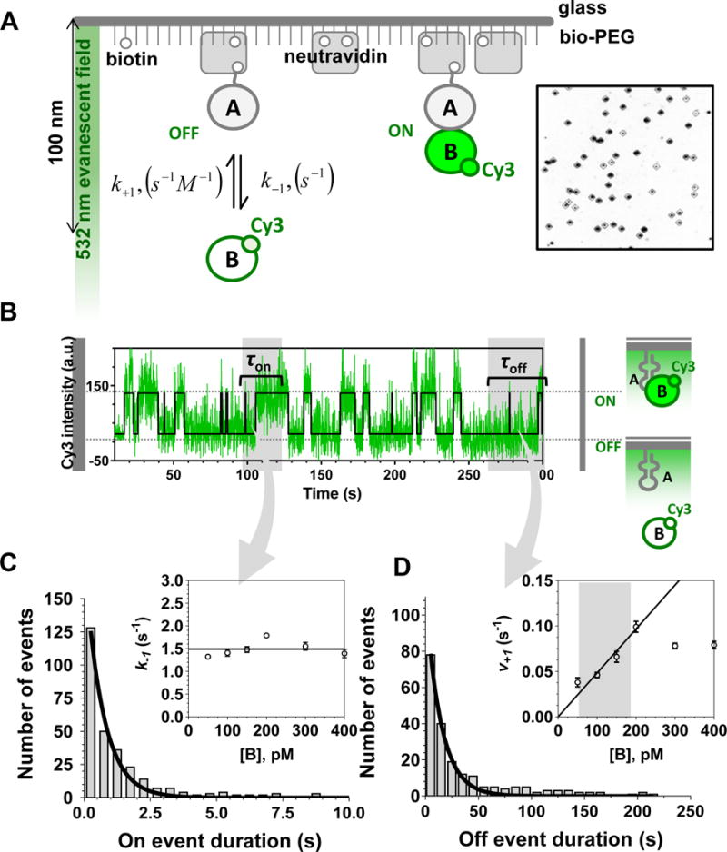
A. The evanescent wave generated by the TIR penetrates the reaction chamber to approximately 100 nm. The biotinylated macromolecules (A) are tethered to the surface of the passified, PEGylated microscope slide via interaction with the neutravidin, which bridges them with the sparsely biotinylated PEG. The Cy3-labeled molecule (B) is then flown into the reaction chamber and the recording is initiated. Formation of the AB complex (governed by the association rate constant k₊₁ and the concentration of freely diffusing B) brings the Cy3-labeled B in the evanescent filed, which excites the dye. Decomposition of the AB complex (governed by the dissociation rate constant k₋₁) leads to diffusion of B away from the evanescent field and in disappearance of the fluorescence signal. The inset shows a part of the camera field of view with dark spots corresponding to the points on the slide where the molecules are tethered and complexes are being formed during the experiment. B. A representative fluorescence trajectory shows the evolution of the Cy3 signal in one of the spots on the slide. Raw data are shown in green overlaid with the idealized trajectory shown as a black line. High Cy3 signal corresponds to the AB complex (τ_on is the “ON” dwell time for the event), while the background fluorescence corresponds to the unbound A (and the corresponding “OFF” dwell time τ_off). The dark grey rectangles in the beginning and at the end of the trajectory indicate the events excluded from the analysis. C. Fitting of the dwell time distribution constructed from all “ON” dwell times with single exponential function provides the dissociation rate constant k₋₁, which is independent of the concentration of B (inset). D. Fitting of the dwell time distribution constructed from all “OFF” dwell times with single exponential function provides the association rate v₊₁, which increases with increasing concentration of B until reaching saturation (inset). The range of the concentrations useful for calculating the association rate constant k₊₁ is marked by the grey rectangle in the inset. The data in this figure are adapted with permission from (Haghighat Jahromi et al., 2013).

2.2.1. Fluorescent nucleic acids

Oligonucleotides (DNA and RNA) can easily be labelled using a modified solid support (CPG) for 3′-modifications or a specialized phosphoramidite reagent for internal and 5′-modifications. DNA and RNA site-specifically labeled with a wide range of fluorophores compatible with most single-molecule TIRFM setups are available for purchase through commercial companies like IDT, MWG Operon, etc.

2.2.2. Fluorescent labeling of proteins

Labeling of proteins can be achieved through several methods depending on the nature of the protein as well as the requirement for site specificity. Direct chemical labeling of proteins involves the reaction of cysteine residues in the protein with maleimide–fluorophore conjugates (GE Healthcare Life Sciences). This reaction is carried out at moderate pH (optimally pH 7) and temperatures. Pretreatment of the protein with a reducing agent (DTT or TCEP) ensures that the cysteine residues are reduced prior to labeling. The presence of several reactive cysteines on the protein may lead to non-homogenous labeling of the protein. One can replace the cysteines whose labeling is not desired with serine or threonine residues providing that this does not affect the structure, the stability, or the activities of the protein. N-terminal labeling of proteins can be carried out using amine reactive dyes such as succinimidyl esters (NHS) like CyDye™ (GE Healthcare Life Sciences) at a neutral pH. At high pH, this method can also be used to selectively label the ε-amino group on lysine residues; however because lysine is a fairly common residue in proteins, this method often leads to heterogeneous labeling, which is undesirable.

A growing number of methods enables site-specific chemical labeling of proteins. The Mycobacterium tuberculosis formyl-glycine generating enzyme (FGE) specifically catalyzes the co-translational oxidation of the cysteine residue on the hexapeptide sequence LCTPSR to an aldehyde containing a Cα-formylglycine (fGly) residue, which can be then labeled in vitro (Appel and Bertozzi, 2015, Liu et al., 2015, Rabuka et al., 2012, Shi et al., 2012, Ghoneim and Spies, 2014). The FGE recognition sequence can be genetically encoded into a protein, which is then co-expressed with FGE, both in eukaryotic as well as prokaryotic expression systems (Rabuka et al., 2012). Fluorescently labeled aminooxy- or hydrazide-functionalized molecules are readily available through GE healthcare (CyDye™ hydrazides) and other companies, which can be used directly in labeling reactions. Alternatively, fluorescence dye can be irreversibly linked to the fGly via a Hydrazinyl-Iso-Pictet-Spengler (HIPS) ligation reaction (Liu et al., 2015). The FGE-mediated labeling is particularly useful when the location of the fluorophore on the protein is critical to observation or when the protein cysteines are important for the activity (Ghoneim and Spies, 2014). As with other labeling strategies, the appropriate controls should be employed to ensure that the addition of the hexapeptide FGE recognition sequence and/or the labeling conditions do not alter the function or activity of the protein of interest.

The sortase system (Theile et al., 2013) is an alternative method that uses the Staphylococcus aureus sortase A enzyme, which recognizes an LPXTG motif in substrate proteins and cleaves the peptide bond between the threonine and glycine residues. A nucleophilic substitution by an α-amine of an incoming oligoglycine-based nucleophile conjugated to a fluorescent dye leads to a modified protein with the fluorophore at the N or C terminus.

2.2.3. Surface-tethering of macromolecules for TIRFM

Surface-tethering is commonly achieved by labeling the protein or nucleic acid with biotin and subsequent immobilization on a neutravidin-coated slide surface. Biotinylated oligonucleotides are readily available from many commercial sources, such as IDT. However, direct biotinylation may be impractical if a long RNA or DNA molecule is used in an experiment. To circumvent this, a biotinylated complementary DNA oligonucleotide can be annealed to a terminus of the RNA or DNA construct, or to an internal region that is not expected to affect the interaction being investigated.

For protein immobilization, a biotin acceptor peptide (BAP) sequence (GLNDIFEAQKIEWHE or 5′ - ggtcttaatgatatttttgaagctcagaagattgaatggcatgaa - 3′) is engineered into the protein expression vector. The BAP is the most efficient recognition sequence for the E. coli BirA biotin ligase, which biotinylates the underlined lysine residue (Beckett et al., 1999). It is typically incorporated at the N- or C-terminus of the protein or, if desired, in a solvent exposed loop. For bacterially expressed proteins, BAP and the presence of 100 μM biotin in the growth media is sufficient for the efficient biotinylation of the target proteins. For proteins expressed in human, baculovirus or yeast cells, the expression system must also contain a vector for the expression of BirA ligase (see (Bain et al., 2016) for a protocol for the expression of biotinylated proteins in human cells, (Honda et al., 2014) for the baculovirus expression, and (Boehm et al., 2016) for the yeast expression).

The biotinylated molecules are immobilized on the surface of the passivated imaging chamber coated with the sparsely biotinylated (1:25) PEG polymer (MPEG-SVA-5000 and Biotin-PEG-SVA-5000, Laysan Bio) and 100 pM – 3 μM neutravidin (Pierce). A detailed protocol describing the imaging chamber construction and preparation of the imaging buffer can be found in (Bain et al., 2016). After a 3 – 5 min incubation, the excess of the untethered molecules are removed from the microscope imaging chamber by washing with the tethering buffer, which is then replaced with the imaging buffer supplemented with the oxygen scavenging system (oxygen scavenging system (1 mg/ml glucose oxidase, 0.4% (w/v) D-glucose, 0.04 mg/mL catalase) and 12 mM Trolox (6-hydroxy-2,5,7,8-tetramethylchromane-2-carboxylic acid), and containing the fluorescently-labeled molecules. The concentration of the biotinylated molecules during the tethering step ranges from 20 – 100 pM; the concentration of the fluorescently labeled molecules in the reaction is typically varied between 50 pM and 1 μM. Higher concentrations of the freely diffusing fluorescent molecules can be measured, but will reduce the signal to noise ratio due to increase in the background fluorescence.

Alternatively, surface-tethering of the proteins can also be achieved through the interaction with a surface-tethered biotinylated antibodies (e.g. biotin-conjugated anti-6xHis, anti-FLAG, or anti-HA antibodies), a technique known as “single-molecule pull down” (SiMPull) (Aggarwal and Ha, 2014, Jain et al., 2012).

For all surface-tethering protocols it is essential to confirm that surface immobilization does not interfere with the biochemical properties of the protein. This can be achieved by carrying out the experiment in an alternative configuration where the surface-tethered and fluorescent molecules are switched.

2.3. Acquisition of binding data

The binding experiment is designed so that the surface-tethered molecules are non-fluorescent and therefore invisible per se. Because of their capacity to bind the freely diffusing, fluorescently-labeled partners their presence on the surface of the TIRFM reaction chamber results in a sequence of high intensity fluorescent events that appear, persist and disappear in a single diffraction-limited spot. The time based-changes in the fluorescence in a designated location is referenced herein as a fluorescence trajectory (Fig. 1B). If surface-tethered molecules are separated further than the diffraction limit (ensured by the low ratio of biotinylated to non-biotinylated PEG molecules and the concentrations of neutravidin and biotinylated molecules during surface immobilization reaction) and in the absence of a non-specific binding, each fluorescence trajectory can be attributed to the binding activity of a single, surface-tethered molecule. Several hundreds of individual trajectories are extracted from each recorded video and visualized using the Single-Molecule FRET data acquisition and analysis suite https://cplc.illinois.edu/software (Joo and Ha, 2012) as described in detail in (Bain et al., 2016). Similar to more established single-molecule FRET measurements, the raw data in single-molecule binding and co-localization studies are first processed using the peak-finder and signal integration algorithms implemented in IDL (Roy et al., 2008, Blanco and Walter, 2010). These algorithms allow one to select molecules from a wide field of view, extract fluorescence trajectories, and, in the case of multi-color imaging, to match the peaks collected in different emission channels.

2.4. Selecting and preparing the trajectories and events for dwell-time analysis

2.4.1. Selection rules

The first step in the analysis of single-molecule trajectories is to establish an unbiased set of selection rules to separate the trajectories for analysis from all extracted trajectories. This allows for an unbiased analysis of the subset of the quality data, as the selection is typically done by eye and may therefore be subjectively biased. For simple one-color measurements of the association of fluorescently-labeled macromolecule with the surface-tethered partner, the main selection criterion is the presence of at least two true binding events, i.e. the events whose dwell-times are longer than 2 frames of the movie and the fluorescence increase is within a minimum predefined threshold of signal to noise ratio. Moreover, to be recorded as a dwell time, the event should start after the beginning of the recording and end before the recording is terminated. For example, the first “OFF” and the last “ON” events in the trajectory shown in Fig. 1B (dark grey rectangles) do not adhere to this criterion and are removed from the analysis. If only one binding event is present in the trajectory, this event can still contribute to the analysis of the “ON” dwell times. Often, it is also advisable to exclude trajectories that show a monotonic decay of intensity of binding events across the total length of the recoded video, and to exclude trajectories that contain events with disproportionally large signal intensity compared to the dominant level of signal intensity in most of the trajectories).

2.4.2. Extracting the dwell times from fluorescence trajectories

Similar to the ion channel open-close transition kinetics (Colquhoun and Sigworth, 1995) and times to completion of the catalytic cycle (Szoszkiewicz et al., 2008, Moffitt et al., 2010), the dwell-times of the molecular association events are computed from the idealized trajectories. When the states are clearly separated and the transitions are obvious, a so-called “thresholding” method may be sufficient for extracting the dwell times that the trajectory spends at each state (Sachs et al., 1982, Zhou et al., 2011, Blanco and Walter, 2010). This description readily applies to the single-molecule binding trajectories where the labeled macromolecule is freely diffusing and is binding to a non-fluorescent surface-tethered partner. For such trajectories, the “bound” (“ON”) state corresponds to a high fluorescence signal and the “free” (“OFF”) state corresponds to background fluorescence level.

When the thresholding method is insufficient, for example, due to the presence of multiple, poorly separated states, or to the noise in the recording, other methods allow better quality idealization, and thereby a more accurate identification of the states and extraction of dwell times (Watkins and Yang, 2005, Bronson et al., 2009, Shuang et al., 2014). A powerful set of methods for extracting kinetic information from noisy trajectories or in the presence of multiple ill-defined states is based on Hidden Markov modelling (HMM) (Chung et al., 1990, Talaga, 2007, Blanco and Walter, 2010, Liu et al., 2010). HMM assumes that the process probed by the single-molecule analysis is a “Markovian”, stochastic, memoryless process in which probability of the next event depends only on the current event and is independent from prior events (Talaga, 2007). Although this assumption is not always true in single-molecule data (Lu et al., 1998), HMM still represents a practical method to identify the various signal states and to quantify the kinetics of transitions between these states (Blanco and Walter, 2010). A detailed and comprehensive description of HMM can be found in (Rabiner, 1989).

There are several HMM-based academic open access programs for idealization of the single-molecule trajectories (McKinney et al., 2006, Greenfeld et al., 2012, van de Meent et al., 2014, Qin and Li, 2004, Nicolai and Sachs, 2013, Bronson et al., 2009). Most of these programs are designed for analyzing single-molecule FRET trajectories, which are calculated from two sets of original trajectories for the FRET donor and the acceptor, respectively. To analyze the non-FRET single-molecule binding data derived from the trajectories exemplified by Fig. 1B we prefer to use the program QuB (“Q” refers to a rate transition matrix, and “UB” refers to University of Buffalo) (Qin and Li, 2004, Nicolai and Sachs, 2013). This software package was originally developed for the analysis of single ion channel recordings. It can idealize multiple trajectories simultaneously and utilizes multi-state models. It also can read data in many different types of formats. Using QuB, one can select a specific part of each trajectory and edit the data that is being analyzed (see sections 2.4.3 and 2.5.5. below). It also can calculate rates and globally fit data obtained under different experimental conditions (e.g. ionic strength, concentrations of freely diffusing macromolecule, etc.). One of the advantages of the QuB package is that it can estimate the likelihood of different models (including all possible connections schemes between states).

When the one-color single molecule data are obtained using a TIRFM system capable of the two-color imaging, Cy5-labeled streptavidin can be utilized to map the positions of biotinylated immobilized molecules on the slide surface.

• Replace neutravidin with the Cy5-labeld streptavidin (GE healthcare PA45001) or use a Cy5-labeled biotinylated target molecule. At the beginning of imaging, use 5 seconds excitation with 640 nm laser, then switch the excitation source to 532 nm laser for the rest of the recording. In this scheme, the MatLab program for extraction of the fluorescence trajectories only needs to consider the first 5 seconds of the recording to map the possible locations of surface-tethered molecules, aiding in the selection of trajectories (Boehm et al., 2016, Haghighat Jahromi et al., 2013). When the unlabeled neutravidin is used for surface-tethering, the MatLab code needs to be set to scan the entire movie in Cy3 channel to identify the locations where the Cy3 signal associated with the binding of the freely diffusing Cy3-labeled ligand appears.

• The portion of the trajectory containing the Cy5 signal is trimmed prior to analysis. We have developed a software tool which allows for the automated removal of this initial Cy5 excitation from the beginning of each trajectory in a given experiment folder (available upon request from Maria Spies or Todd Washington). The software will automatically truncate all files in a given folder, at a given row number and will save the updated file. Fig. 1B shows the trajectory after trimming to remove the Cy5 label.

• The trajectories for a given single molecule experiment are then individually analyzed using QuB (Nicolai and Sachs, 2013). The one-color fluorescence trajectories are fit to a two-state model, wherein the “OFF” times are denoted as “0” and the “ON” times are denoted as “1 or on”. The “Amps” function in QuB is used to calculate the average values for both a low fluorescence population and a high fluorescence population for each individual trajectory. The “Idealize” command then identifies binding events utilizing these low and high fluorescence values, such that increases in fluorescence which are within one standard deviation of the average value for the high fluorescence population and persist for two or more consecutive camera frames will be identified as binding events. Increases in fluorescence signal which do not meet these requirements are considered noise and are ignored. An idealized data trajectory is then generated (Fig. 1B) along with the idealized data file containing durations e of all “ON” and “OFF” events in a given trajectory in order of appearence.

• The QuB idealized data are then input into Microsoft Excel for further analysis (the automated software tool for the batch processing of QuB output files is available on request from Maria Spies or Todd Washington). This software opens each idealized QuB data file within a given folder, identifying them by the file extension .qwt and copies and pastes the information into the Excel document with a line between each idealized file to identify the trajectory number that it originated from. Binding events whose beginning or whose end are truncated by the recording window of the movie (dark grey rectangles in the trajectory in Fig. 1B) are automatically omitted from analysis. Trajectories which have only one binding event are marked to be used only for consideration of the “ON” dwell time. The data are then sorted into “ON” times (given the designation of 1 by QuB) and “OFF” times (given the designation of 0 by QuB). The “ON” and “OFF” dwell time data are then used in the histogram construction and kinetic analysis as described below in section 2.5.

2.4.3. Errors introduced into observed binding kinetics due to the fluorophore blinking and photo-bleaching

Reversible blinking (Rasnik et al., 2006, Valeur, 2012) and irreversible photo-bleaching of fluorescent dyes (Diaspro; A, 2006, Lakowicz, 2006) are photo-physical phenomena frequently observed in single-molecule fluorescence imaging experiments. In the case of blinking, the fluorescent dye visits a dark non-emissive state, stays in this state for some time (usually micro-seconds to milli-seconds (Akyuz et al., 2013, Bartley et al., 2003)), then returns to the electronic ground state and restarts the cycles of excitation and emissive de-excitation. Photo-bleaching is a process in which the dye encounters a photochemical reaction that leads to complete loss of its emissive property. Both phenomena are comprehensively discussed in a recent review (Ha and Tinnefeld, 2012). After a fluorescently-labeled freely-diffusing macromolecule binds to its surface-tethered partner (“ON”-state), its dissociation (indicated by the decrease in the fluorescence signal to the background level) can be confused with blinking or photo-bleaching (especially when dissociation is slow and the dwell times are long). Hence, blinking and photo-bleaching can introduce significant errors in the evaluation of rate of any process studied by the single-molecule fluorescence imaging (Bartley et al., 2003, Rueda et al., 2004). To determine that the fluorophore blinking or photo-bleaching does not affect a single-molecule binding experiment, we recommend the following routine:

• Select the lowest possible laser excitation intensity that provides acceptable signal-to-noise ratio sufficient for extracting reliable kinetics (Haller et al., 2011).

• Measure the photo-bleaching time (τ_bleach) of the fluorescent dye at the chosen excitation laser intensity using an immobilized form of the same fluorescently-labeled macromolecule by plotting the distribution of lengths of the fluorescence trajectories and then fitting this distribution to an exponential function (Solomatin et al., 2010). Using the same fluorescently-labeled species is important because the dye photo-physics is influenced by its chemical environment (Bartley et al., 2003).

• Carry out the binding experiment. Repeat the acquisition of the single-molecule binding data at least one more time, but using higher excitation intensity.

• Compare the binding kinetics (i.e. dwell time distributions) evaluated from the data acquired using the two different excitation laser intensities.

• If no dependence on excitation intensity was observed, then this means that blinking and photo-bleaching did not induce significant errors in the observed binding kinetics. Using the current photostabilizing and oxygen scavenging strategies (Zheng et al., 2014, Ha and Tinnefeld, 2012), many recent single-molecule binding studies showed no significant errors induced in the observed binding kinetics due to blinking or photo-bleaching.

• In some cases, significant errors can still be introduced into the observed binding kinetics. This can be due to more than one reason; it can be because the dissociation rate is relatively slow which makes data acquisition limited by photo-bleaching (Honda et al., 2014), or because the fluorescence emission quantum yield of the dye is significantly reduced upon attachment to the target macromolecule sample, which consequently forces the experimenter to use very high excitation laser intensity in order to collect data with sufficient signal to noise ratio.

• If the observed kinetics shows laser intensity dependence, it may be influenced by (i) both blinking & photo-bleaching; (ii) photo-bleaching only; or (iii) blinking only.

• In the first scenario, binding dwell time distributions are expected to be of multiphasic nature; with one shorter phase whose fraction/amplitude and time constant depend on excitation intensity but does not depend on perturbations related to the biochemical reaction under study (e.g. ionic strength, etc.), and another longer phase whose time constant depends on both the biochemical reaction perturbations and excitation laser intensity. The former is usually due to blinking, while the later originates from the binding/assembly process but has also a photo-bleaching associated error.

• In the second scenario, binding dwell time distributions should be monophasic (i.e. can be fit to single exponential model).

• In the third scenario, binding dwell time distributions should be again multiphasic, but in this case the time constant of the longer phase does not depend on excitation laser intensity, although it depends on the biochemical reaction perturbations.

The procedures for accounting for the errors induced due to these photo-physical phenomena are described in detail in the next section.

2.5. Construction and analysis of the dwell time distributions

2.5.1. Presenting the dwell time data as ordinary frequency and cumulative distributions

To make meaningful inferences into the mechanisms of biomolecular interactions, it is usually not enough to merely observe the binding events in the single-molecule trajectories. While every individual trajectory is unique, reflecting a stochastic nature of the macromolecular collisions and binding, the overall statistical properties extracted from a large collection of trajectories reflect on the macroscopic behavior of the process under investigation. The theory behind constructing, fitting and statistical analysis of dwell-time distributions developed for the single-channel recording data (Colquhoun and Sigworth, 1995) has been applied to analysis of many different single-molecule systems (Munro et al., 2007, Abelson et al., 2010, Szoszkiewicz et al., 2008). Collectively, the single-molecule binding data may be presented as the histograms of the observed dwell times. Two types of the distributions are most commonly used, ordinary or frequency distributions and cumulative distributions. Frequency distributions are constructed by plotting the number (or frequency) of the dwell times that fell in a certain time interval (bin) vs. time (Fig. 1 C&D, Fig. 2 A&E). The resulting histogram can then be compared to a theoretical probability density function describing the process (e.g. exponential or multiple exponential). When normalized for the size of the data set, height of each bin defines the probability that a random dwell time falls within a particular interval. In cumulative distributions, the value on the y-axis represents the sum of all events that had a dwell time between zero and a corresponding time. When normalized, the cumulative distribution defines the probability that a random dwell time falls below a given value. The number of points in the exact cumulative distribution is equal to the number of observed dwell times, which is especially useful for smaller data sets (see the discussion below).

Fig. 2. Construction and analysis of the dwell time distributions.

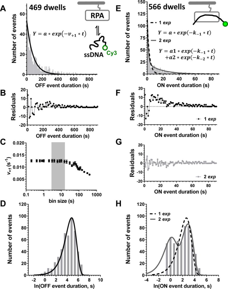
The data in this figure are adapted with permission from (Chen et al., 2016). A. A histogram of the 469 individual “OFF” dwell times for the complex formation between the surface-tethered RPA protein and a Cy3-labeled 30-mer ssDNA constructed using 10 seconds bins (grey bars) is fitted with a single-exponential function (black line). B. The residuals from the fit shown in A display a symmetric scatter around zero. C. The same data set was binned with varying bin size and fitted with single exponential function. The resulting association rate is plotted as a function of bin size. It remains the same between the minimal reasonable bin size of 200 milliseconds to about 20 seconds. Larger bin size combines most of the data in a very few bins (the half-life for this process is around 55 seconds) and consequently to an erroneous determination of the rate. The grey rectangle suggests the optimal bin size range. D. The same data are plotted on the logarithmic scale. E. A histogram of the 566 individual “ON” dwell times for the RPA-ssDNA constructed using 1 second bins (grey bars) is fitted with a single-exponential function (black dashed line) and double exponential (grey continuous line). F. The residuals from the single-exponential fit shown in D display a systematic deviation from zero. G. The residuals from the double-exponential fit display a symmetric scatter around zero and are much tighter. H. The same data are plotted on the logarithmic scale clearly reveal that the process is indeed a double exponential. The grey rectangle shows the values missing due to the slow sampling rate.

2.5.2. Selecting a bin size of the ordinary frequency histogram

Presenting the dwell time data as frequency histograms requires the large data sets (hundreds to thousands of data points) to yield accurate rate constants. Not surprisingly, the distributions built from a smaller number of dwell times show the greatest sensitivity to the effects of binning. The rules for the unbiased, objective choice of the optimal bin size have evolved from the historically earliest Sturges’ rule (1926) to a number of more recent mathematical rules (Wand, 1997, Sturges, 1926, Shimazaki and Shinomoto, 2007, Doane, 1976, Scott, 1979). However, the main problem with these rules of optimal bin size selection is that they are based on assumptions with regard to the nature of the distribution. Ideally, optimal bin size calculation should be model-independent, such as in the method developed by Shinomoto & Shimazaki (Shimazaki and Shinomoto, 2007). In this method, the bin size associated with the minimum mean integrated squared error (MISE) is the optimal one. The MISE is calculated directly from the data, and the method is available as a web application at http://toyoizumilab.brain.riken.jp/hideaki/res/histogram.html. The only assumption in this method is that data are sampled independently of each other. Later this method was updated (Shimazaki and Shinomoto, 2010) to be able to find optimal bin width in case of a processes whose rates change over time (e.g. binding of two macromolecules, with one of them switching during the same trajectory between multiple conformers that have different association and dissociation rates). In our experience, this method requires very large data set for the best performance. Even with the data set sizes in the range of few hundred dwell times, the calculated optimal bin size did not permit good fitting of a multiphasic dwell time distribution to multi-exponential function because significant amount of the data was spread over the longer side of the scale (unpublished results).

Practically, the optimum bin size depends on the number of recorded observations, the spread of the data, and the overall shape of the distribution. While the smaller bin size improves the accurate determination of the rate constants, the small number of events in narrow bins will result in a noisy signal that may be difficult to fit. Moreover, the 30 ms or 100 ms camera resolution used in our experiments provides the uncertainty in determining the beginning and the end of each event; i.e. if the camera resolution is set for 100 ms, and the threshold for recognizing the event in QuB is set as at least two consecutive frames, a bin size less than 200 ms is not meaningful. Intuitively, the bin size should be selected so that more than two bins are present before the half point of the fast phase of the exponential decay fitted to the distribution. This is because an ordinary frequency histogram is built of multiples of a sampling interval and the bin heights at the middle of each bin should approximate the probability density function for the distribution. This approximation becomes poor when the bin width approaches or exceeds the time constant of the probability density function. If the bin size is too large, it may skew the fitting, i.e. all meaningful data will be combined in a single bin, and the respective rate constants (the overall rate constant for a single exponential distribution or the constant describing the rapid phase of the process) will be inaccurate. Fig. 2C provides an illustration how the association rate determined from the fitting of the “OFF” time distribution of the RPA-ssDNA complexation (Chen et al., 2016) is affected by the change in the bin size. In this particular case, the calculated rate remains the same until the bin size starts exceeding 20 seconds, which is about a half of a half-life of the distribution.

2.5.3. Logarithmic histograms

One disadvantage of the ordinary histogram is that the bins containing the long dwell times have very few data points. The rare long events that may carry important biological consequences may therefore be overlooked during the fitting (Honda et al., 2014). It may also be difficult to unambiguously determine whether the distribution is monophasic (i.e. can be fit by a single exponential function) or multiphasic. When distinguishing between single and multiple processes from the linear dwell time distribution is problematic, the distribution can be replotted as a logarithmic histogram (Fig. 2D&H). Note that it is sometime advantageous to use a square root ordinate instead of the histogram with logarithmic x-axis and linear y-axis depicted in Fig. 2D&H. Numerous reports from the ion channel field (Sigworth and Sine, 1987, McManus et al., 1987) and more recent single-molecule work (Szoszkiewicz et al., 2008) showed that logarithmic histograms can robustly discriminate between the processes characterized by a single rate vs. multiple rates. Another advantage of log-dwell time histogram is that it is more suitable in case of data with range that covers multiples scales (e.g. from micro-seconds to 10’s of seconds) (Colquhoun and Sigworth, 1995). Fig. 2D&H shows the data from Fig. 2A&E plotted on the logarithmic scale. Because the bins of such a histogram contain logarithmic values of the dwell time durations, the bins for longer and shorter times are better balanced. Recently, Fernandez and colleagues suggested a method to achieve two targets at the same time: (i) evaluating optimal bin size and (ii) judging whether a process should be described with single or multiple rates (Szoszkiewicz et al., 2008). This method is based on combining logarithmic time abscissa type of histogram with using reduced χ² as an objective bin size estimation parameter. An optimal bin size can be determined through an iterative process starting from the smallest reasonable bin size. For each iteration, the bin size is increased, the resulting distribution is fitted and the reduced χ² is calculated. The χ² value decreases with the increase in the bin size until it reaches a global minimum or levels off (Szoszkiewicz et al., 2008). It is worth mentioning that this method depends on the model (e.g. single exponential or multi-exponential function) that the experimenter uses to calculate the reduced χ² value for each bin size tested.

2.5.4. Cumulative distributions

Both, linear and logarithmic histograms require large data sets (i.e. several hundreds to several thousands of data points) to yield accurate rate constants. Not surprisingly, the distributions built from a smaller number of dwell-times show the greatest sensitivity to the effects of binning. Cumulative representation of distributions helps to solve a great deal of this problem (Sung et al., 2010). In addition, it avoids the complexities associated with finding the optimal bin size, as it is independent of binning (Gebhardt et al., 2006). One of the common forms of the cumulative distribution displays the fraction of dwell times that are longer than a given time “t” (Sung et al., 2010, Ghoneim and Spies, 2014, Strick et al., 2000). Each event in this type of representation is given an equal weight, which increases the ratio of data points to parameters allowing for more robust analysis (Sung et al., 2010) and increases the weight of the rare long events (Bartley et al., 2003). Cumulative representations of dwell time distributions are especially useful for estimation of the number of rate constants. However, care must be taken when using this representation of distributions (Friedman and Gelles, 2015). Successive points in this type of data representation are correlated, which may bias curve fitting (Colquhoun and Sigworth, 1995). Least-squares fitting of cumulative distributions using commercial software may lead to an underestimation of fit uncertainty if the software did not consider covariance of fit parameters (Sung et al., 2010), and if an independent error in successive points on the graph is assumed (Friedman and Gelles, 2015). It is suggested that fitting cumulative distributions using maximum-likelihood methods combined with an estimation of fit uncertainty using a bootstrapping method can provide a more reliable strategy to evaluate rates of processes from single-molecule data. In the bootstrapping approach, a data set identical in size to the original data set is constructed by randomly selecting the dwell times with replacement, and the new dataset is fitted to obtain the rate constants. The process is repeated several hundred times. The average for the resulting set of values for each rate constant and the standard deviation are then used to assess the quality of the fit.

2.5.5. Correcting the observed rates for the fluorophore photo-bleaching and blinking

Several methods allow one to correct for the photo-bleaching errors. In one popular method, the photo-bleaching rate (inverse of τ_bleach) is subtracted from the observed rate to calculate the actual corrected rate (Miyanaga and Ueda, 2011, Watanabe and Mitchison, 2002, Honda et al., 2014, Rueda et al., 2004). Another method uses a semi-empirical approach where the relation between change in the observed dissociation rate is plotted versus the change in laser exposure time, using the same excitation intensity and period of data recording (Huppa et al., 2010, Friedman and Gelles, 2015, Bombardier et al., 2015). Assuming a linear dependence of these two parameters, actual binding kinetics can be evaluated by extrapolating the curve to zero laser exposure.

Errors associated with blinking are more difficult to handle. Some studies ignore the fast, laser power dependent component of the dwell time distributions (Akyuz et al., 2013). In these studies, the slower phase of the dwell time distribution is used to measure the rate of the process after confirming that the time constant of this phase depends on biochemical perturbations (e.g. changing the ionic strength). A data-screening method was developed in other studies (Bartley et al., 2003, Rueda et al., 2004). Here, the fluorescent dye is immobilized, so that the sudden decrease in fluorescence signal to background level is due to blinking only, not because of dissociation from the surface of the microscope slide. The kinetics of blinking of the dye is then characterized. By combining this rough characterization of the blinking kinetics with a selection criteria related to emission intensity, a sub-population of short dark intervals in the trajectories is ignored, then the analysis of dynamics of fluctuations of fluorescence trajectories is repeated and the dwell time distributions are reconstructed and re-fitted. It is important to note that the design of the selection criteria mentioned above differs from one experimental system to another.

2.5.6. Mechanistic interpretation of the rates obtained from the dwell-time distributions

Finding the best fitting probability distribution of the single-molecule data does not automatically generate a reasonable model of the actual process under investigation. For a sufficiently large data set, a mathematical shape of a distribution function can be identified by curve fitting followed up by a statistical analysis as exemplified by the two cases above. To understand the underlying molecular process, however, it is essential to explain the shape of a given distribution function by an underlying generative principle. Many macromolecular association processes discussed in this chapter are simple Poissonian process with a single dominant energy barrier. As result, their respective probability density functions are single-exponentials (see for example the dwell time distributions for both “ON” and “OFF” dwell times in Fig. 1C&D and the “OFF” time distribution in Fig. 2A). Similar to the bulk associated kinetics described by Debye-Smoluchowski equation, the probability of the surface-tethered molecule to form an observable complex or the frequency of appearance of the fluorescent signal in a particular location on the microscope slide (reflected in the “OFF” time distributions) is proportional to the frequency of the collisions between the molecule on the surface and the freely diffusing counterpart adjusted by a unitless factor that accounts for the fraction of productive collisions. If the “OFF” time distribution deviates from single exponential, this may signify the presence of distinct subpopulations of conformers or distinct subpopulations among the surface-tethered molecules with distinct binding properties. The “ON” time distribution reflects stability of the complex, which in the case of a homogenous system decomposes in a single step leading to a single-exponential distribution. Multiple exponentials are frequently observed and are likely to reflect the formation of distinct complexes with different stabilities (Amrute-Nayak et al., 2014, Chen et al., 2016) (Fig. 2E).

2.5.7. Interaction stoichiometry

If the fluorescent labeling is homogenous (i.e. all freely diffusing molecules contain no more than a single dye) and only the 1:1 complexes are formed, each binding event generates a signal of similar intensity, and the process can be model as two-state, “bound” (“ON”) and “free” (“OFF”). More complex binding patterns can be observed if the surface-tethered molecule contains multiple binding sites for the fluorescently-labeled binding partner(s), which may bind independently or oligomerize upon binding to the surface-tethered substarte. An example of the interaction involving multiple independent binding sites can be found in a study examining the interaction of muscleblind-like 1 protein (MBNL1) with RNA molecules containing CUG repeats (Haghighat Jahromi et al., 2013). The protein bound the surface-tethered (CUG)₄ construct with 1:1 stoichiometry. In contrast, more complex trajectories were observed with the (CUG)₁₂ construct, and the intensity histograms suggested the presence of 3 independent binding sites for MBNL1 on this RNA, reflecting the expectation for the etiology of the Myotonic dystrophy type 1 where MBNL1 is sequestered by the (CUG)_n repeats transcribed from the expanded (CAG)_n repetitive DNA. The presence of multiple binding sites on the surface tethered macromolecule does not necessarily complicate the analysis of macromolecular complexation as it would in the analogous bulk experiment. This is because each binding event is observed independently at sufficiently low concentration of the fluorescently-labeled freely diffusing molecules. Another elegant study by Pond and colleagues (Pond et al., 2009) is an example of the single-molecule enabled analysis that revealed oligomerization of the protein on the nucleic acid. This study probed the stoichiometry and the mechanism of assembly of the HIV-1 Rev protein on the Rev Response Element (RRE), a highly conserved region of the viral mRNA. The intensity histograms assembled from ~1,000 individual 20 sec trajectories and subjected to Hidden Markov analysis using HAMMY program (McKinney et al., 2006) showed the presence of 4 distinct bound states with 1 to 4 Rev proteins bound to the RRE RNA. The stepwise changes in the fluorescence intensity revealed the sequential addition and dissociation of the monomer from the RNA with higher-order complex formation on the RRE RNA driven primarily by protein-protein interaction.

3. Binary interactions in the presence of inhibitors

3.1. Inhibitors of macromolecular interactions

Even in its simplest one-color version, TIRFM-based single-molecule co-localization provides a suite of powerful approaches to develop a comprehensive understanding of the inhibition mechanism and the kinetics of the macromolecular interactions in the presence of an inhibitor (Haghighat Jahromi et al., 2013). In this section we provide a guide on how to design and carry this type of analysis. We will use a study of the non-competitive inhibition of the interaction between muscleblind-like 1 protein (MBNL1) and the CUG repeat containing RNA (Haghighat Jahromi et al., 2013), but the overall approach can be generally applied to competitive and non-competitive inhibitors, as well as the allosteric effectors of protein-protein and protein nucleic acid interactions. The major advantage of this approach is that it is model-independent, i.e. we do not need to assume the mechanism a priori. The ability to detect and measure the individual binding events in real time and under the equilibrium conditions at multiple inhibitor concentrations provides all the information one needs to not only access the inhibitor potency, but also to infer its mechanism of action.

The overall experimental scheme starts from establishing and optimizing the conditions for the analysis of macromolecular interaction (as described in section 2).

• One of the interacting molecules should be biotinylated for surface tethering, and the other fluorescently labeled and freely diffusing. The inhibitor (effector) is unlabeled and should not have significant absorbance or fluorescence in the experimental excitation/emission windows. If the inhibitor produces a significant signal that interferes with the observation of the binding trajectories, we recommend labeling the freely diffusing macromolecule with a fluorophore whose spectral properties do not overlap with those of the inhibitor. This will require using a different laser for the excitation along with optimizing the excitation and emission filters.

• If feasible, the system should be selected or simplified to ensure a 1:1 binding stoichiometry. In the case of the MBNL1-RNA interaction, for example, we determined that a stem-loop RNA (5′-bio-GCUGCUGUGCGCUGCUG-3′), referred herein as (CUG)₄, provides a minimal substrate to which a single MBNL1 molecule binds with the affinity similar to that of the expanded CUG repeats. Moreover, this RNA molecule is expected to form a 1:1 complex with the bioactive dimeric inhibitor, which the study investigated (Haghighat Jahromi et al., 2013).

• The conditions are then established and optimized for collecting the fluorescence binding trajectories and for extracting the most reliable on and off rates, respective rate constants and the equilibrium dissociation constant.

• The binding experiments are then repeated at several concentrations of the inhibitor. The range of the inhibitor concentrations should be greater than twice the expected K_i (equilibrium inhibition constant for the competitive inhibitor or K_D (equilibrium dissociation constant for the inhibitor-target complex). For example, for the inhibitor which binds (CUG)₄ with K_D =2.9 ± 0.2 μM, we carried out the single-molecule binding reactions in the presence of 0, 0.5. 1, 2, 4, and 6 μM inhibitor, while 0, 4, 20, 100, 200 μM inhibitor was used in the case of another compound whose affinity for (CUG)₄ was 71 ± 27 μM.

• The “ON” and “OFF” dwell times are extracted from the fluorescence trajectories as described above, binned and plotted as ordinary frequency distributions, which are then globally fitted to determine the rate and equilibrium constants and the inhibition mechanism (see below).

3.2. Determining the inhibition mechanism: competitive inhibition

Competitive inhibitors (Fig. 3A) compete with the ligand (B) by occupying the same site on the target macromolecule (A). In the experimental scheme outlined in Fig. 3A, macromolecule A is tethered to the surface, B is fluorescently labeled and is free in solution, and I is a competitive inhibitor that binds A. In the absence of the inhibitor, formation of the A-B complex is observed as the appearance of fluorescence signal. A competitive inhibitor should have no effect on the “ON” dwell time distributions and therefore on the dissociation rate constant k₋₁. In contrast, while the A-I complex is undetectable on its own, its formation precludes A-B complexation resulting in reduced frequency of binding events, and eventually no detectable binding at high inhibitor concentrations. When detectable, the distributions of the “OFF” dwell times will remain single exponential

$$Y=a\ast \mathit{\text{exp}}(-v_{+1}^{\mathit{\text{obs}}}\ast t),$$ (eq. 3.1)

where $v_{+1}^{\mathit{\text{obs}}}$ is the observed association rate at the chosen inhibitor concentration [I].

$$v_{+1}^{\mathit{\text{obs}}}=v_{+1}\frac{[B]}{K_D\left(1+\frac{[I]}{K_i}\right)+[B]},$$ (eq. 3.2)

where K_i is the inhibition constant that reflect the affinity of the inhibitor for A, $K_D=\frac{k_{-1}}{k_{+1}}$ is the affinity of the ligand B for A, and [B] is the concentration of freely diffusing fluorescently-labeled B in the reaction chamber. Constant a allows to fit the distribution without the need for normalization and accounts for all binding events, including those too short to be detected due to the temporal resolution of the measurement. If the inhibitor is determined to be competitive, there are two possible procedures to obtain the K_i. One can choose to fit the “OFF” time distributions at each inhibitor concentration individually using the equation 3.1, plot the observed association rate as a function of [I] and fit the resulting graph using the equation 3.2. The accurate determination of K_i in this case requires at least 5 $v_{+1}^{\mathit{\text{obs}}}$ values in the broad range of the inhibitor concentrations. Alternatively, one can determine K_D from the binding experiments in the absence of the inhibitor, and then globally fit the “OFF” time distribution from several inhibitor concentrations to the combined equation

$$Y=a\ast \mathit{\text{exp}}\left(-v_{+1}\frac{[B]}{K_D\left(1+\frac{[I]}{K_i}\right)+[B]}\ast t\right)$$ (eq. 3.3)

where K_i is a shared value for all data sets, and a is unique for each set allowing to globally fit the distributions without normalization. Note that there is no need to select the same bin size or the same size of the data set for each distribution.

Fig. 3. Single-molecule analysis of the binary macromolecular interactions in the presence of unlabeled inhibitors.

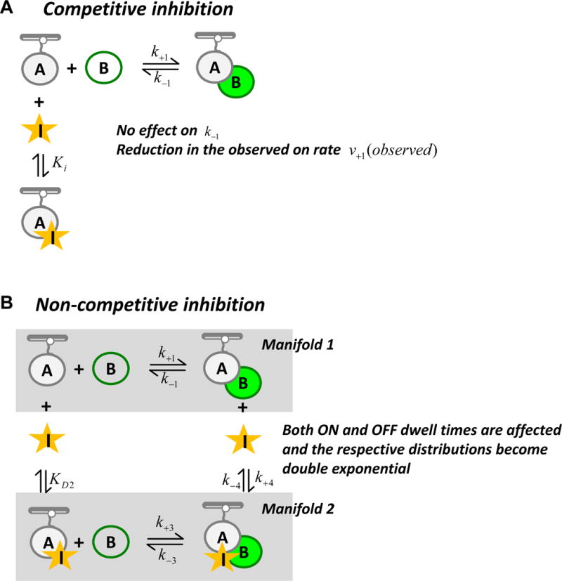
A. Competitive inhibition. The experimental scheme is essentially the same as in the single-molecule analysis of binary interaction. The inhibitor that interacts with A is depicted as a star. K_i is the equilibrium inhibition constant. B. Non-competitive inhibition. Both A-B and A-B-I complexes are observed.

3.3. Unlabeled ligand as a competitive inhibitor

Using an unlabeled macromolecule as a competitive inhibitor may be used to determine if labeling affects its affinity for the surface-tethered partner. We recommend carrying out the binding reaction at several concentrations of the unlabeled molecule and analyzing them as described in the section 3.2. If labeling has no effect on the affinity, the calculated K_i will be equal K_D; if K_i > K_D, the labeling has negative effect on the binding affinity.

Labeling of the macromolecules for single-molecule analysis is not always 100% efficient, and the freely diffusing species contain a mixture of labeled and unlabeled molecules of B. If this is the case, an accurate determination of the binding properties by single-molecule TIRFM is still possible. If both labeled and unlabeled species display the same binding properties, the actual association rate can be calculated from the observed rate as

$$v_{+1}=\frac{v_{+1}^{\mathit{\text{obs}}}+\sqrt{{\left(v_{+1}^{\mathit{\text{obs}}}\right)}^2+4\alpha v_{+1}^{\mathit{\text{obs}}}{k}_{-1}}}{2\alpha [B]}$$ (eq. 3.4)

where α is a fraction of labeled B. The binding analysis here should be carried out in the linear range of the association rate dependence of [B].

3.4. Determining the inhibition mechanism: non-competitive inhibition

In a more complex non-competitive inhibition scenario, a ternary complex A-B-I containing the inhibitor, ligand and the target molecule may form (Fig. 3B). This complex is expected to have a different stability from the A-B complex and may be assembled by either binding of the ligand to the A-I complex, or by binding of the inhibitor to the A-B complex. Similarly, the A-B-I complex may decompose to either A-B or A-I complexes. The presence of the non-competitive inhibitor does not completely abolish the A-B complex formation at any concentration, and both the “ON” and “OFF” dwell times are affected. For simplicity, we will consider a scenario where, in the absence of the inhibitor, both “ON” and “OFF” dwell time distributions fit well to the single exponential functions. The kinetic scheme for the reaction in the presence of noncompetitive inhibitor and all relevant rate constants are depicted in Fig. 3B. Appearance of the fluorescent signal in the single-molecule trajectories in this case may signify the formation of the A-B complex by binding of B to the surface-tethered A (k₊₁), or by the formation of A-B-I complexes by binding of B to the A-I complex (k₊₃). The interconversion between A-B and A-B-I complexes (k₊₄ and k₋₄, respectively) is not detected, nor does binding of I to A (the affinity if I for A is defined by K_D2; respective rate constants cannot be determined from this analysis). Similarly, A-B-I may decompose to A-I with the rate constant k₋₃, which is observed as a loss of the signal. A-B-I decomposition may also proceed through the A-B complex, which then dissociates with the rate constant k₋₁.

• The binding experiments are carried out as described in the section 3.1. in the presence of multiple concentration of the non-competitive inhibitor.

• The “OFF” time data are then binned and plotted as ordinary frequency distributions, which will have a double exponential shape.

• The “OFF” dwell time distributions for all inhibitor concentrations are globally fit to the following equation:

  $$Y=A[K_{D2}\mathit{\text{exp}}(-k_{+1}[B]t)+[I]\mathit{\text{exp}}(-k_{+3}[B]t)]$$ (eq. 3.5)

  where k₊₁ is obtained from the analysis of A-B complexation in the absence of the inhibitor, K_D2 is a shared value for all data sets and the constant is allowed to vary to reflect different sizes of the datasets at different inhibitor concentrations. A ∗ K_D2 is the weight of manifold (1) whereas A ∗ [I] is the weight of manifold (2) adjusted by the number of observed events. See (Haghighat Jahromi et al., 2013) for the detailed explanations and the full list of the assumptions underlying this analysis.
• Similarly, the “ON” dwell time distributions are globally fit to equation:

  $$Y=A[K_{D2}\mathit{\text{exp}}(-(k_{-1}-k_{+4}[I]t)+[I]\mathit{\text{exp}}(-(k_{-3}-k_{-4})t)]$$ (eq. 3.6)

  yielding K_D2, k₊₄ and (k₋₃ − k ₋₄). Parameters k₋₃ and k₋₄ are linked as (k₋₃ − k₋₄) and therefore cannot be determined individually by fitting but can be calculated from the linked equilibria as $k_{-3}=\frac{(k_{-3}-k_{-4})k_{+3}{K}_{D1}}{k_{+3}{K}_{D1}-k_{+4}{K}_{D2}}$

This analysis was initially developed to describe and compare the two inhibitors of the MBNL1 binding to the CUG repeat containing RNA (Haghighat Jahromi et al., 2013), but may be readily extended to the analysis of any non-competitive inhibitors of the macromolecular assembly.

While powerful and straight forward in their implementation, the analysis detailed in this section fail to address the kinetics of the inhibitor-target interaction. We show above how to obtain the K_I and K_D2, but not individual k₊₂ and k₋₂. To directly access these parameters, the smTIRFM study may be complemented by an SPR (surface plasmon resonance) experiment, which follows the kinetics of the inhibitor binding to the surface-tethered target molecule and detects the A-I complex formation in a label-independent manner. Availability of the biotinylated macromolecule developed for the smTIRFM studies greatly streamlines setting up the SPR experiment.

In some cases, the competitor is macromolecule (nucleic acid or protein) that can be fluorescently labeled and binds to the target molecule with sufficiently high affinity to be compatible with the single-molecule TIRFM experiment. Such a competitor may be analyzed using two-color imaging scheme described in the next section.

4. Co-localization by single-molecule total internal reflection fluorescence microscopy

4.1. TIRFM-enabled co-localization single-molecule imaging of binding processes

Single-molecule optical co-localization at a physiologically relevant temperature is a powerful method that can be dated to mid-1990’s (Funatsu et al., 1995). It can be achieved using many types of imaging modes or configurations (Enderle et al., 1997, Schutz et al., 1998, Churchman et al., 2005, Selvin et al., 2008, Uemura et al., 2010, Friedman and Gelles, 2012). Conceptually, it also includes techniques like single-molecule FRET (Ha et al., 1996). Here we will specifically focus on single-molecule co-localization binding studies (with diffusion in 2D or/and 3D) using TIRFM, in the absence of FRET or any type of quenching (Boehm, 2016, Friedman et al., 2006, Koyama-Honda et al., 2005). In a co-localization experiment, one has to obtain multiple spectrally distinct images of the same field of view (FOV), and, in the excitation pathway, the illumination fields of multiple wavelengths should overlap in space. Ideally, fluorophores should be selected so that they (i) have a minimal spectral overlap (to minimize signal leakage between the channels) and (ii) are of a comparable photophysical properties, such as photo-bleaching rates, blinking dynamics and emission quantum yield. Co-localization can be achieved using multiple emission collection schemes, for example; (i) single detector (e.g. CCD camera) whose sensor area spatially split into multiple sections (i.e. channels) recording signals from multiple dyes simultaneously, (ii) single detector alternatingly and quickly recording signals from multiple dyes, (iii) multiple detectors, each one recording signal from one dye separately (see (Roy et al., 2008, Selvin et al., 2008, Larson et al., 2014) for comprehensive reviews). During analysis of videos, mathematical mapping is used to identify corresponding locations in all detection channels (Friedman and Gelles, 2015, Ghoneim and Spies, 2014, Roy et al., 2008). False positives (i.e. detection of co-localized spots when they are not actually present) is minimized using a combination of optimum mapping and spot detection algorithms. A practical tip to minimize false negatives is to use comparable excitation rates for all fluorophores so that emission rates are also comparable in addition to the selecting dyes with similar photophysical properties.

4.2. Detecting binary and ternary complexes with two-color imaging

This section will focus on two-color fluorescent imaging, which affords the direct visualization of two fluorescently labeled macromolecules binding to a non-fluorescent, immobilized macromolecule. These studies can be particularly informative when studying the architecture of the ternary complexes formed by these three macromolecules, as well as the kinetics of the assembly and disassembly of these complexes. This approach will be illustrated with a recent example in which the formation and dynamics of the ternary complexes that form among the translesion synthesis proteins DNA polymerase eta (pol η), Rev1, and proliferating cell nuclear antigen (PCNA) was studied (Boehm, 2016). In these experiments, biotinylated pol η was immobilized on the surface of a quartz slide and the binding of Cy3-labeled PCNA and Cy5-labeled Rev1 to pol η was observed.

The binding events involving single immobilized pol η molecules are represented as fluorescence trajectories with time on the x-axis and fluorescence intensity on the y-axis (Fig. 4A). Cy3-labeled PCNA fluorescence is shown in green and Cy5-labeled Rev1 fluorescence is shown in red. Baseline fluorescence levels signify that no proteins are bound to the immobilized pol η molecule. An increase in Cy3 fluorescence above the baseline indicates the binding of PCNA to pol η, and an increase in Cy5 fluorescence indicates Rev1 binding. Likewise, a decrease in fluorescence back to the baseline indicates the dissociation of either PCNA or Rev1 from pol η. In this sample trajectory, there are five binding events: three events (2, 3, and 5) are binary complexes in which Cy5-labeled Rev1 binds to pol η and two events (1 and 4) contain ternary complexes in which Cy3-labeled PCNA and Cy5-labeled Rev1 simultaneously bind to pol η. Binding events truncated by the beginnings or the endings of the recordings are omitted from analysis because the exact timing of Cy3-PCNA or Cy5-Rev1 association or dissociation cannot be determined.

Fig. 4. Single-molecule analysis of ternary macromolecular complexes.

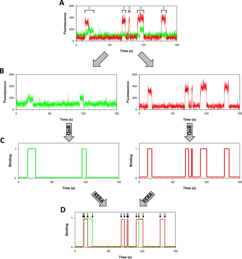
The data in this figure are adapted with permission from (Boehm, 2016) A, Sample fluorescence trajectory shows the evolution of the Cy3 (green) and Cy5 (red) signals in one of the spots on the slide. High Cy3 signal corresponds to the PCNA binding to the immobilized pol η molecule. High Cy5 signal represents Rev1 bound to the immobilized pol η. The five binding events are indicated. B, The Cy3 and Cy5 signals are separated into two trajectories. C, Idealized Cy3 and Cy5 trajectories are obtained from QuB. D, the idealized Cy3 and Cy5 trajectories are re-combined and analyzed by KERA.

4.3 Kinetic event resolving algorithm (KERA)

Using two-color fluorescence imaging experiments, one can observe the formation of a variety of binary and ternary complexes. Thus, it is necessary to categorize the individual binding events. Because of the size of these single molecule data sets, it is helpful to automate the categorization process in order to promote more rapid and efficient analysis. We have developed software in the form of a plug-in for Microsoft Excel for categorizing binding events from two-color fluorescence imaging experiments, which we have named kinetic event resolving algorithm (KERA).

The fluorescence trajectories from the two channels, Cy3 and Cy5, are analyzed separately by QuB to identify the Cy3 and Cy5 binding events (Fig. 4B,C). The two normalized, idealized trajectories corresponding to a given immobilized macromolecule are then recombined by KERA (Fig. 4D). The binding events for each channel are imported and enumerated in a table, which contains the beginning time, ending time, and duration of each Cy3 and Cy5 binding event. KERA then examines the binding events in the Cy3 channel and determines whether there are coincident binding events in the Cy5 channel utilizing the Index function in Excel. If there is no coincident binding, then any events that occur are categorized as Cy3 binding only or Cy5 binding only binary events.

If there is coincident binding, KERA executes a series of logic statements to classify the binding event. We will use the first binding event in the idealized trajectory shown in Fig. 4D as an example of how KERA classifies binding events. In this example, we have four transitions (indicated by arrows). The first transition occurs at time t=15.3 seconds and corresponds to the binding of a Cy5-labeled Rev1 to the immobilized pol η to form a pol η-Rev1 binary complex. The second transition occurs at time t=17.1 seconds and corresponds to the binding of a Cy3-labeled PCNA to form a pol η-Rev1-PCNA ternary complex. The next transition occurs at time t=22.7 seconds and corresponds to the dissociation of the Cy5-labeled Rev1 leaving a pol η-PCNA binary complex. The final transition occurs at time t=30.6 seconds and corresponds to the dissociation of Cy3-labeled PCNA from the immobilized pol η. Table 4.1 shows the logic statements that KERA applies in order to categorize these binding events.

Table 4.1.

Categorization of binding events by KERA

Event	Logical Statement	Event Classification	Duration, s
1	at t=15.3 (Cy3=0, Cy5=1) AND at t=17.1 (Cy3=1, Cy5=1) AND at t=22.7 (Cy3=1, Cy5=0) AND at t=30.6 (Cy3=0, Cy5=0)	Cy5 binding first and Cy5 dissociating first	15.3
2	at t=81.8 (Cy3=0, Cy5=1) AND at t=88.5 (Cy3=0, Cy5=0)	Cy5 binding only	6.7
3	at t=93.8 (Cy3=0, Cy5=1) AND at t=95.4 (Cy3=0, Cy5=0)	Cy5 binding only	1.6
4	at t=109.2 (Cy3=0, Cy5=1) AND at t=114.4 (Cy3=1, Cy5=1) AND at t=120.6 (Cy3=0, Cy5=0)	Cy5 binding first and Cy3 and Cy5 dissociating simultaneously	11.4
5	at t=152.4 (Cy3=0, Cy5=1) AND at t=160.3 (Cy3=0, Cy5=0)	Cy5 binding only	7.9

By applying such logic statements to all Cy3 and Cy5 binding data, KERA categorizes events into one of the following eleven categories (Fig. 5). Two of these are binary complexes:

• a)Cy3 binding only
• b)Cy5 binding only

Fig. 5. Idealized trajectories of binary and ternary complexes.

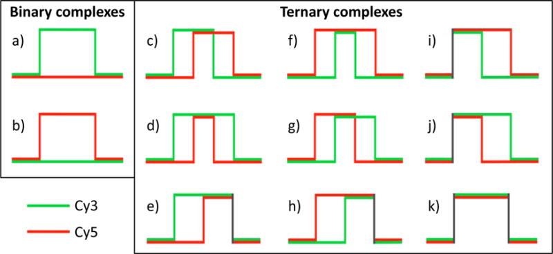
Idealized trajectories of (a) the binary complex between Cy3-labeled PCNA binding to pol η and (b) the binary complex between Cy5-labeled Rev1 binding to pol η. Idealized trajectories of (c) the ternary complex in which Cy3-labeled PCNA binds pol η first and the Cy3-labeled PCNA releases from pol η first, (d) the ternary complex in which Cy3-labeled PCNA binds pol η first and the Cy5-labeled Rev1 releases from pol η first (i.e., the hallmark of a PCNA tool belt), (e) the ternary complex in which Cy3-labeled PCNA binds pol η first and both proteins release from pol η simultaneously, (f) the ternary complex in which Cy5-labeled Rev1 binds pol η first and the Cy3-labeled PCNA releases from pol η first (i.e., the hallmark of a Rev1 bridge), (g) the ternary complex in which Cy5-labeled Rev1 binds pol η first and the Cy5-labeled Rev1 releases from pol η first, (h) the ternary complex in which Cy5-labeled Rev1 binds pol η first and both proteins release from pol η simultaneously, (i) the ternary complex in which both proteins bind pol η simultaneously and Cy3-labeled PCNA releases from η first, (j) the ternary complex in which both proteins bind pol η simultaneously and Cy5-labeled Rev1 releases from η first, (k) the ternary complex in which both proteins bind pol η simultaneously and both proteins release from η simultaneously.

Nine of these are ternary complexes:

• c)Cy3 binding first and Cy3 dissociating first
• d)Cy3 binding first and Cy5 dissociating first
• e)Cy3 binding first and Cy3 and Cy5 dissociating simultaneously
• f)Cy5 binding first and Cy3 dissociating first
• g)Cy5 binding first and Cy5 dissociating first
• h)Cy5 binding first and Cy3 and Cy5 dissociating simultaneously
• i)Cy3 and Cy5 binding simultaneously and Cy3 dissociating first
• j)Cy3 and Cy5 binding simultaneously and Cy5 dissociating first
• k)Cy3 and Cy5 binding simultaneously and Cy3 and Cy5 dissociating simultaneously

KERA can be expanded to categorize and analyze data from more complicated experimental systems. Additional fluorescence channels can be added to analyze the formation of higher order complexes (quaternary, quinary, etc.). Because KERA was built using VBA in Microsoft Excel, it is an approachable and intuitive software tool to both use and edit for a variety of applications. KERA is available upon request from Maria Spies and Todd Washington.

4.4 Determining the order of assembly and architecture of multi-component complexes

We used two-color fluorescence imaging experiments combined with an analysis facilitated by KERA to study the architecture and dynamics of the ternary complex that forms between the translesion synthesis proteins pol η, Rev1, and PCNA (Boehm, 2016). The interaction between pol η and PCNA and the interaction between pol η and Rev1 are both mediated by the pol η (PCNA-interacting protein) PIP motif. Consequently, pol η cannot directly bind to both PCNA and Rev1 simultaneously. This implies that the architectures of the ternary complexes formed by these three proteins must be either “PCNA tool belts” or “Rev1 bridges” (Fig. 6). In a PCNA tool belt, pol η directly interacts with PCNA and PCNA directly interacts with Rev1, but pol η and Rev1 do not directly interact. In a Rev1 bridge, pol η directly interacts with Rev1 and Rev1 directly interacts with PCNA, but pol η and PCNA do not directly interact. The architecture of individual ternary complexes can be deduced in several ways.

Fig. 6. Types of binary and ternary complexes.

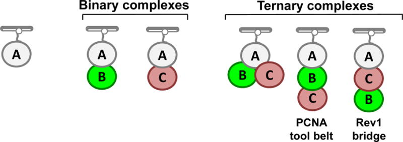
Binary complexes are shown between A and B and between A and C. Ternary complexes are shown among A, B, and C. In the first ternary complex (left), B and C both simultaneously bind A. In the second (middle), A directly binds B and B directly binds C, but A does not directly bind C. When A is pol η, B is PCNA, and C is Rev1, this arrangement is a PCNA tool belt. In the third (right) A directly binds C and C directly binds B, but A does not directly bind B. When A is pol η, B is PCNA, and C is Rev1, this arrangement is a Rev1 bridge.

One way to determine the architecture of each ternary complex is by examining their order of assembly and disassembly. For example, if the immobilized pol η first binds PCNA to form a PCNA-pol η binary complex and then this binary complex binds Rev1 to form a ternary complex, one can conclude that the ternary complex assembles as a PCNA tool belt. By contrast, if pol η first binds Rev1 and then binds PCNA, one can conclude that the resultant ternary complex assembles as a Rev1 bridge. Likewise, if Rev1 first dissociates from a ternary complex leaving behind a pol η-PCNA binary complex and then PCNA dissociates next, one can conclude that the ternary complex disassembled as a PCNA tool belt. Lastly, if PCNA dissociates first from a ternary complex and Rev1 dissociates next, one can conclude that the ternary complex dissembled as a Rev1 bridge.

We observed approximately 1,000 ternary complexes formed by Cy3-labeled PCNA, Cy5-labeled Rev1, and immobilized, unlabeled pol η. Based on their orders of assembly and disassembly, we found that about 40 % of the ternary complexes were PCNA tool belts and roughly 20 % were Rev1 bridges. We were unable to unambiguously determine the architecture of about 20 % of the ternary complexes. This was because PCNA and Rev1 bound pol η together as a pre-formed complex obscuring their order of assembly or because both PCNA and Rev1 dissociated from pol η together obscuring their order of disassembly. Surprisingly, we found that approximately 10 % of the ternary complexes assembled as a PCNA tool belt but disassembled as a Rev1 bridge and that about 10 % of the complexes assembled as a Rev1 bridge but disassembled as a PCNA tool belt. This suggests that these ternary complexes are dynamic and are capable of switching architectures (from a PCNA tool belt to a Rev1 bridge and vice versa) without any proteins dissociating from the complex.

Another way to determine the architecture of a ternary complex is to use mutant proteins that are defective in binding one of the other binding partners. For example, the interaction between pol η and Rev1 requires the C-terminal domain (CTD) of Rev1. We made a series of amino acid substitutions in the Rev1 CTD that interfere with the ability of Rev1 to bind pol η, but not the ability of Rev1 to bind PCNA. As a result, mutant Rev1 protein would be unable to engage in the formation of Rev1 bridges, but will not interfere with the formation of PCNA tool belts. When identical two-color fluorescence imaging experiments were carried out with this mutant Rev1 protein, we observed a greatly reduced number of Rev1 bridges, but not PCNA tool belts. Studies with mutant proteins such as these can help unambiguously define the architecture ternary complexes.

5. Conclusions and future outlook

Single-molecule fluorescence microscopy is emerging as a powerful tool for the analysis of the dynamic assembly of various molecular machines. The smTIRFM-enabled workflow for the analysis presented in this chapter illustrates the power of this straight forward single-molecule assay to provide a comprehensive mechanistic description of macromolecular interactions ranging in scope from the binary interactions, to the formation and dynamics of ternary complexes, to the application of single-molecule fluorescence to study the inhibitors of protein-protein and protein-nucleic acid interactions. We discussed general considerations of the experimental design, controls, and data acquisition and analysis.

Analysis of the assembly and dynamics of larger multicomponent complexes, and the ability to combine multi-color imaging with studies of the inhibitors will require further development of more complicated data analysis routines as well as the experimental schemes that will allow one to evaluate the sources of heterogeneity. The basic routines, however, are in place and hopefully will become as common in the tool box of many biophysicists and biochemists as structural biology approaches and pre-steady state kinetics analysis are today.

References

- ABELSON J, BLANCO M, DITZLER MA, FULLER F, ARAVAMUDHAN P, WOOD M, VILLA T, RYAN DE, PLEISS JA, MAEDER C, GUTHRIE C, WALTER NG. Conformational dynamics of single pre-mRNA molecules during in vitro splicing. Nat Struct Mol Biol. 2010;17:504–12. doi: 10.1038/nsmb.1767. [DOI] [PMC free article] [PubMed] [Google Scholar]
- AGGARWAL V, HA T. Single-molecule pull-down (SiMPull) for new-age biochemistry: methodology and biochemical applications of single-molecule pull-down (SiMPull) for probing biomolecular interactions in crude cell extracts. Bioessays. 2014;36:1109–19. doi: 10.1002/bies.201400090. [DOI] [PubMed] [Google Scholar]
- AKYUZ N, ALTMAN RB, BLANCHARD SC, BOUDKER O. Transport dynamics in a glutamate transporter homologue. Nature. 2013;502:114–8. doi: 10.1038/nature12265. [DOI] [PMC free article] [PubMed] [Google Scholar]
- AMRUTE-NAYAK M, LAMBECK KA, RADOCAJ A, HUHNT HE, SCHOLZ T, HAHN N, TSIAVALIARIS G, WALTER WJ, BRENNER B. ATP turnover by individual myosin molecules hints at two conformers of the myosin active site. Proc Natl Acad Sci U S A. 2014;111:2536–41. doi: 10.1073/pnas.1316390111. [DOI] [PMC free article] [PubMed] [Google Scholar]
- APPEL MJ, BERTOZZI CR. Formylglycine, a post-translationally generated residue with unique catalytic capabilities and biotechnology applications. ACS Chem Biol. 2015;10:72–84. doi: 10.1021/cb500897w. [DOI] [PMC free article] [PubMed] [Google Scholar]
- AXELROD D. Chapter 7: Total internal reflection fluorescence microscopy. Methods Cell Biol. 2008;89:169–221. doi: 10.1016/S0091-679X(08)00607-9. [DOI] [PubMed] [Google Scholar]
- BAIN FE, WU CG, SPIES M. Single-molecule sorting of DNA helicases. Methods. 2016 doi: 10.1016/j.ymeth.2016.05.009. [DOI] [PMC free article] [PubMed] [Google Scholar]
- BARTLEY LE, ZHUANG X, DAS R, CHU S, HERSCHLAG D. Exploration of the transition state for tertiary structure formation between an RNA helix and a large structured RNA. J Mol Biol. 2003;328:1011–26. doi: 10.1016/s0022-2836(03)00272-9. [DOI] [PubMed] [Google Scholar]
- BECKETT D, KOVALEVA E, SCHATZ PJ. A minimal peptide substrate in biotin holoenzyme synthetase-catalyzed biotinylation. Protein Sci. 1999;8:921–9. doi: 10.1110/ps.8.4.921. [DOI] [PMC free article] [PubMed] [Google Scholar]
- BLANCO M, WALTER NG. Analysis of complex single-molecule FRET time trajectories. Methods Enzymol. 2010;472:153–78. doi: 10.1016/S0076-6879(10)72011-5. [DOI] [PMC free article] [PubMed] [Google Scholar]
- BOEHM EM, POWERS KT, KONDRATICK CM, SPIES M, HOUTMAN JC, WASHINGTON MT. The Proliferating Cell Nuclear Antigen (PCNA)-interacting Protein (PIP) Motif of DNA Polymerase eta Mediates Its Interaction with the C-terminal Domain of Rev1. J Biol Chem. 2016;291:8735–44. doi: 10.1074/jbc.M115.697938. [DOI] [PMC free article] [PubMed] [Google Scholar]
- BOEHM EM, SPIES M, WASHINGTON MT. PCNA tool belts and polymerase bridges form and interconvert in translesion synthesis complexes. Nucleic Acids Research (in revision) 2016 doi: 10.1093/nar/gkw563. [DOI] [PMC free article] [PubMed] [Google Scholar]
- BOMBARDIER JP, ESKIN JA, JAISWAL R, CORREA IR, JR, XU MQ, GOODE BL, GELLES J. Single-molecule visualization of a formin-capping protein ‘decision complex’ at the actin filament barbed end. Nat Commun. 2015;6:8707. doi: 10.1038/ncomms9707. [DOI] [PMC free article] [PubMed] [Google Scholar]
- BRONSON JE, FEI J, HOFMAN JM, GONZALEZ RL, JR, WIGGINS CH. Learning rates and states from biophysical time series: a Bayesian approach to model selection and single-molecule FRET data. Biophys J. 2009;97:3196–205. doi: 10.1016/j.bpj.2009.09.031. [DOI] [PMC free article] [PubMed] [Google Scholar]
- CHEN J, ZHANG Z, LI L, CHEN BC, REVYAKIN A, HAJJ B, LEGANT W, DAHAN M, LIONNET T, BETZIG E, TJIAN R, LIU Z. Single-molecule dynamics of enhanceosome assembly in embryonic stem cells. Cell. 2014;156:1274–85. doi: 10.1016/j.cell.2014.01.062. [DOI] [PMC free article] [PubMed] [Google Scholar]
- CHEN R, SUBRAMANYAM S, ELCOCK AH, SPIES M, WOLD MS. Dynamic binding of replication protein a is required for DNA repair. Nucleic Acids Res. 2016 doi: 10.1093/nar/gkw339. [DOI] [PMC free article] [PubMed] [Google Scholar]
- CHUNG SH, MOORE JB, XIA LG, PREMKUMAR LS, GAGE PW. Characterization of single channel currents using digital signal processing techniques based on Hidden Markov Models. Philos Trans R Soc Lond B Biol Sci. 1990;329:265–85. doi: 10.1098/rstb.1990.0170. [DOI] [PubMed] [Google Scholar]
- CHURCHMAN LS, OKTEN Z, ROCK RS, DAWSON JF, SPUDICH JA. Single molecule high-resolution colocalization of Cy3 and Cy5 attached to macromolecules measures intramolecular distances through time. Proc Natl Acad Sci U S A. 2005;102:1419–23. doi: 10.1073/pnas.0409487102. [DOI] [PMC free article] [PubMed] [Google Scholar]
- COLQUHOUN D, SIGWORTH F. Fitting and Statistical Analysis of Single-Channel Records. In: SAKMANN B, NEHER E, editors. Single-Channel Recording. Plenum Press; New York: 1995. [Google Scholar]
- DIASPRO A, C G, USAI C, RAMOINO P, DOBRUCKI J. Photobleaching. In: PAWLEY J, editor. Handbook of Biological Confocal Microscopy. Third. Springer Science+Business Media, LLC; 2006. [Google Scholar]
- DOANE DP. Aesthetic frequency classification. American Statistician. 1976;30:181–183. [Google Scholar]
- ELENKO MP, SZOSTAK JW, VAN OIJEN AM. Single-molecule imaging of an in vitro-evolved RNA aptamer reveals homogeneous ligand binding kinetics. J Am Chem Soc. 2009;131:9866–7. doi: 10.1021/ja901880v. [DOI] [PMC free article] [PubMed] [Google Scholar]
- ENDERLE T, HA T, OGLETREE DF, CHEMLA DS, MAGOWAN C, WEISS S. Membrane specific mapping and colocalization of malarial and host skeletal proteins in the Plasmodium falciparum infected erythrocyte by dual-color near-field scanning optical microscopy. Proc Natl Acad Sci U S A. 1997;94:520–5. doi: 10.1073/pnas.94.2.520. [DOI] [PMC free article] [PubMed] [Google Scholar]
- FRIEDMAN LJ, CHUNG J, GELLES J. Viewing dynamic assembly of molecular complexes by multi-wavelength single-molecule fluorescence. Biophys J. 2006;91:1023–31. doi: 10.1529/biophysj.106.084004. [DOI] [PMC free article] [PubMed] [Google Scholar]
- FRIEDMAN LJ, GELLES J. Mechanism of transcription initiation at an activator-dependent promoter defined by single-molecule observation. Cell. 2012;148:679–89. doi: 10.1016/j.cell.2012.01.018. [DOI] [PMC free article] [PubMed] [Google Scholar]
- FRIEDMAN LJ, GELLES J. Multi-wavelength single-molecule fluorescence analysis of transcription mechanisms. Methods. 2015;86:27–36. doi: 10.1016/j.ymeth.2015.05.026. [DOI] [PMC free article] [PubMed] [Google Scholar]
- FUNATSU T, HARADA Y, TOKUNAGA M, SAITO K, YANAGIDA T. Imaging of single fluorescent molecules and individual ATP turnovers by single myosin molecules in aqueous solution. Nature. 1995;374:555–9. doi: 10.1038/374555a0. [DOI] [PubMed] [Google Scholar]
- GEBHARDT JC, CLEMEN AE, JAUD J, RIEF M. Myosin-V is a mechanical ratchet. Proc Natl Acad Sci U S A. 2006;103:8680–5. doi: 10.1073/pnas.0510191103. [DOI] [PMC free article] [PubMed] [Google Scholar]
- GHONEIM M, SPIES M. Direct correlation of DNA binding and single protein domain motion via dual illumination fluorescence microscopy. Nano Lett. 2014;14:5920–31. doi: 10.1021/nl502890g. [DOI] [PMC free article] [PubMed] [Google Scholar]
- GREENFELD M, PAVLICHIN DS, MABUCHI H, HERSCHLAG D. Single Molecule Analysis Research Tool (SMART): an integrated approach for analyzing single molecule data. PLoS One. 2012;7:e30024. doi: 10.1371/journal.pone.0030024. [DOI] [PMC free article] [PubMed] [Google Scholar]
- HA T, ENDERLE T, OGLETREE DF, CHEMLA DS, SELVIN PR, WEISS S. Probing the interaction between two single molecules: fluorescence resonance energy transfer between a single donor and a single acceptor. Proc Natl Acad Sci U S A. 1996;93:6264–8. doi: 10.1073/pnas.93.13.6264. [DOI] [PMC free article] [PubMed] [Google Scholar]
- HA T, TINNEFELD P. Photophysics of fluorescent probes for single-molecule biophysics and super-resolution imaging. Annu Rev Phys Chem. 2012;63:595–617. doi: 10.1146/annurev-physchem-032210-103340. [DOI] [PMC free article] [PubMed] [Google Scholar]
- HAGHIGHAT JAHROMI A, HONDA M, ZIMMERMAN SC, SPIES M. Single-molecule study of the CUG repeat-MBNL1 interaction and its inhibition by small molecules. Nucleic Acids Res. 2013;41:6687–97. doi: 10.1093/nar/gkt330. [DOI] [PMC free article] [PubMed] [Google Scholar]
- HALLER A, RIEDER U, AIGNER M, BLANCHARD SC, MICURA R. Conformational capture of the SAM-II riboswitch. Nat Chem Biol. 2011;7:393–400. doi: 10.1038/nchembio.562. [DOI] [PubMed] [Google Scholar]
- HONDA M, OKUNO Y, HENGEL SR, MARTIN-LOPEZ JV, COOK CP, AMUNUGAMA R, SOUKUP RJ, SUBRAMANYAM S, FISHEL R, SPIES M. Mismatch repair protein hMSH2-hMSH6 recognizes mismatches and forms sliding clamps within a D-loop recombination intermediate. Proc Natl Acad Sci U S A. 2014;111:E316–25. doi: 10.1073/pnas.1312988111. [DOI] [PMC free article] [PubMed] [Google Scholar]
- HOSKINS AA, RODGERS ML, FRIEDMAN LJ, GELLES J, MOORE MJ. Single molecule analysis reveals reversible and irreversible steps during spliceosome activation. Elife. 2016;5 doi: 10.7554/eLife.14166. [DOI] [PMC free article] [PubMed] [Google Scholar]
- HUPPA JB, AXMANN M, MORTELMAIER MA, LILLEMEIER BF, NEWELL EW, BRAMESHUBER M, KLEIN LO, SCHUTZ GJ, DAVIS MM. TCR-peptide-MHC interactions in situ show accelerated kinetics and increased affinity. Nature. 2010;463:963–7. doi: 10.1038/nature08746. [DOI] [PMC free article] [PubMed] [Google Scholar]
- JAIN A, LIU R, XIANG YK, HA T. Single-molecule pull-down for studying protein interactions. Nat Protoc. 2012;7:445–52. doi: 10.1038/nprot.2011.452. [DOI] [PMC free article] [PubMed] [Google Scholar]
- JOO C, HA T. Single-molecule FRET with total internal reflection microscopy. Cold Spring Harb Protoc. 2012;2012 doi: 10.1101/pdb.top072058. [DOI] [PubMed] [Google Scholar]
- JOSHI CP, PANDA D, MARTELL DJ, ANDOY NM, CHEN TY, GABALLA A, HELMANN JD, CHEN P. Direct substitution and assisted dissociation pathways for turning off transcription by a MerR-family metalloregulator. Proc Natl Acad Sci U S A. 2012;109:15121–6. doi: 10.1073/pnas.1208508109. [DOI] [PMC free article] [PubMed] [Google Scholar]
- KOYAMA-HONDA I, RITCHIE K, FUJIWARA T, II, NO R, MURAKOSHI H, KASAI RS, KUSUMI A. Fluorescence imaging for monitoring the colocalization of two single molecules in living cells. Biophys J. 2005;88:2126–36. doi: 10.1529/biophysj.104.048967. [DOI] [PMC free article] [PubMed] [Google Scholar]
- LAKOWICZ J. Single-Molecule Detection. In: LAKOWICZ J, editor. Principles of Fluorescence Spectroscopy. Third. Springer Science+Business Media, LLC; 2006. [Google Scholar]
- LARSON J, KIRK M, DRIER EA, O’BRIEN W, MACKAY JF, FRIEDMAN LJ, HOSKINS AA. Design and construction of a multiwavelength, micromirror total internal reflectance fluorescence microscope. Nat Protoc. 2014;9:2317–28. doi: 10.1038/nprot.2014.155. [DOI] [PMC free article] [PubMed] [Google Scholar]
- LIU J, HANNE J, BRITTON BM, SHOFFNER M, ALBERS AE, BENNETT J, ZATEZALO R, BARFIELD R, RABUKA D, LEE JB, FISHEL R. An Efficient Site-Specific Method for Irreversible Covalent Labeling of Proteins with a Fluorophore. Sci Rep. 2015;5:16883. doi: 10.1038/srep16883. [DOI] [PMC free article] [PubMed] [Google Scholar]
- LIU Y, PARK J, DAHMEN KA, CHEMLA YR, HA T. A comparative study of multivariate and univariate hidden Markov modelings in time-binned single-molecule FRET data analysis. J Phys Chem B. 2010;114:5386–403. doi: 10.1021/jp9057669. [DOI] [PubMed] [Google Scholar]
- LU HP, XUN L, XIE XS. Single-molecule enzymatic dynamics. Science. 1998;282:1877–82. doi: 10.1126/science.282.5395.1877. [DOI] [PubMed] [Google Scholar]
- MCKINNEY SA, JOO C, HA T. Analysis of single-molecule FRET trajectories using hidden Markov modeling. Biophys J. 2006;91:1941–51. doi: 10.1529/biophysj.106.082487. [DOI] [PMC free article] [PubMed] [Google Scholar]
- MCMANUS OB, BLATZ AL, MAGLEBY KL. Sampling, log binning, fitting, and plotting durations of open and shut intervals from single channels and the effects of noise. Pflugers Arch. 1987;410:530–53. doi: 10.1007/BF00586537. [DOI] [PubMed] [Google Scholar]
- MIYANAGA Y, UEDA M. Single-Molecule Kinetic Analysis of Stochastic Signal Transduction Mediated by G-Protein Coupled Chemoattractant Receptors. In: SAKO Y, UEDA M, editors. Cell Signaling Reactions: Single-Molecular Kinetic Analysis. 1st. Springer Science+Business Media B. V; 2011. [Google Scholar]
- MOFFITT JR, CHEMLA YR, BUSTAMANTE C. Methods in statistical kinetics. Methods Enzymol. 2010;475:221–57. doi: 10.1016/S0076-6879(10)75010-2. [DOI] [PubMed] [Google Scholar]
- MUNRO JB, ALTMAN RB, O’CONNOR N, BLANCHARD SC. Identification of two distinct hybrid state intermediates on the ribosome. Mol Cell. 2007;25:505–17. doi: 10.1016/j.molcel.2007.01.022. [DOI] [PMC free article] [PubMed] [Google Scholar]
- NICOLAI C, SACHS F. Solving Ion Channel Kinetics with the QuB Software. Biophysical Reviews and Letters. 2013;8:1–21. [Google Scholar]
- POND SJ, RIDGEWAY WK, ROBERTSON R, WANG J, MILLAR DP. HIV-1 Rev protein assembles on viral RNA one molecule at a time. Proc Natl Acad Sci U S A. 2009;106:1404–8. doi: 10.1073/pnas.0807388106. [DOI] [PMC free article] [PubMed] [Google Scholar]
- QIN F, LI L. Model-based fitting of single-channel dwell-time distributions. Biophys J. 2004;87:1657–71. doi: 10.1529/biophysj.103.037531. [DOI] [PMC free article] [PubMed] [Google Scholar]
- RABINER L. A Turorial on Hidden Markov Models and Selected Applications in Speech Recognition. Proceeding of the IEEE. 1989;77:257–286. [Google Scholar]
- RABUKA D, RUSH JS, DEHART GW, WU P, BERTOZZI CR. Site-specific chemical protein conjugation using genetically encoded aldehyde tags. Nat Protoc. 2012;7:1052–67. doi: 10.1038/nprot.2012.045. [DOI] [PMC free article] [PubMed] [Google Scholar]
- RASNIK I, MCKINNEY SA, HA T. Nonblinking and longlasting single-molecule fluorescence imaging. Nat Methods. 2006;3:891–893. doi: 10.1038/nmeth934. [DOI] [PubMed] [Google Scholar]
- ROY R, HOHNG S, HA T. A practical guide to single-molecule FRET. Nat Methods. 2008;5:507–16. doi: 10.1038/nmeth.1208. [DOI] [PMC free article] [PubMed] [Google Scholar]
- RUEDA D, BOKINSKY G, RHODES MM, RUST MJ, ZHUANG X, WALTER NG. Single-molecule enzymology of RNA: essential functional groups impact catalysis from a distance. Proc Natl Acad Sci U S A. 2004;101:10066–71. doi: 10.1073/pnas.0403575101. [DOI] [PMC free article] [PubMed] [Google Scholar]
- SACHS F, NEIL J, BARKAKATI N. The automated analysis of data from single ionic channels. Pflugers Arch. 1982;395:331–40. doi: 10.1007/BF00580798. [DOI] [PubMed] [Google Scholar]
- SCHUTZ GJ, TRABESINGER W, SCHMIDT T. Direct observation of ligand colocalization on individual receptor molecules. Biophys J. 1998;74:2223–6. doi: 10.1016/S0006-3495(98)77931-7. [DOI] [PMC free article] [PubMed] [Google Scholar]
- SCOTT DW. On optimal and data-based histograms. Biometrika. 1979;66:605–610. [Google Scholar]
- SELVIN P, LOUGHEED T, HOFFMAN M, PARK H, BALCI H, BLEHM B, TOPRAK E. In vitro and in vivo FIONA and other acronyms for watching molecular motors walk. In: SELVIN P, HA T, editors. Single-Molecule Techniques. Cold Spring Harbor Laboratory Press; 2008. [Google Scholar]
- SHI X, JUNG Y, LIN LJ, LIU C, WU C, CANN IK, HA T. Quantitative fluorescence labeling of aldehyde-tagged proteins for single-molecule imaging. Nat Methods. 2012;9:499–503. doi: 10.1038/nmeth.1954. [DOI] [PMC free article] [PubMed] [Google Scholar]
- SHIMAZAKI H, SHINOMOTO S. A method for selecting the bin size of a time histogram. Neural Comput. 2007;19:1503–27. doi: 10.1162/neco.2007.19.6.1503. [DOI] [PubMed] [Google Scholar]
- SHIMAZAKI H, SHINOMOTO S. Kernel bandwidth optimization in spike rate estimation. J Comput Neurosci. 2010;29:171–82. doi: 10.1007/s10827-009-0180-4. [DOI] [PMC free article] [PubMed] [Google Scholar]
- SHUANG B, COOPER D, TAYLOR JN, KISLEY L, CHEN J, WANG W, LI CB, KOMATSUZAKI T, LANDES CF. Fast Step Transition and State Identification (STaSI) for Discrete Single-Molecule Data Analysis. J Phys Chem Lett. 2014;5:3157–3161. doi: 10.1021/jz501435p. [DOI] [PMC free article] [PubMed] [Google Scholar]
- SIGWORTH FJ, SINE SM. Data transformations for improved display and fitting of single-channel dwell time histograms. Biophys J. 1987;52:1047–54. doi: 10.1016/S0006-3495(87)83298-8. [DOI] [PMC free article] [PubMed] [Google Scholar]
- SOLOMATIN SV, GREENFELD M, CHU S, HERSCHLAG D. Multiple native states reveal persistent ruggedness of an RNA folding landscape. Nature. 2010;463:681–4. doi: 10.1038/nature08717. [DOI] [PMC free article] [PubMed] [Google Scholar]
- STRICK TR, CROQUETTE V, BENSIMON D. Single-molecule analysis of DNA uncoiling by a type II topoisomerase. Nature. 2000;404:901–4. doi: 10.1038/35009144. [DOI] [PubMed] [Google Scholar]
- STURGES HA. The Choice of a Class Interval. Journal of the American Statistical Association. 1926;21:65–66. [Google Scholar]
- SUNG J, SIVARAMAKRISHNAN S, DUNN AR, SPUDICH JA. Single-molecule dual-beam optical trap analysis of protein structure and function. Methods Enzymol. 2010;475:321–75. doi: 10.1016/S0076-6879(10)75014-X. [DOI] [PubMed] [Google Scholar]
- SZOSZKIEWICZ R, AINAVARAPU SR, WIITA AP, PEREZ-JIMENEZ R, SANCHEZ-RUIZ JM, FERNANDEZ JM. Dwell time analysis of a single-molecule mechanochemical reaction. Langmuir. 2008;24:1356–64. doi: 10.1021/la702368b. [DOI] [PubMed] [Google Scholar]
- TALAGA DS. COCIS: Markov processes in single molecule fluorescence. Curr Opin Colloid Interface Sci. 2007;12:285–296. doi: 10.1016/j.cocis.2007.08.014. [DOI] [PMC free article] [PubMed] [Google Scholar]
- THEILE CS, WITTE MD, BLOM AE, KUNDRAT L, PLOEGH HL, GUIMARAES CP. Site-specific N-terminal labeling of proteins using sortase-mediated reactions. Nat Protoc. 2013;8:1800–7. doi: 10.1038/nprot.2013.102. [DOI] [PMC free article] [PubMed] [Google Scholar]
- UEMURA S, AITKEN CE, KORLACH J, FLUSBERG BA, TURNER SW, PUGLISI JD. Real-time tRNA transit on single translating ribosomes at codon resolution. Nature. 2010;464:1012–7. doi: 10.1038/nature08925. [DOI] [PMC free article] [PubMed] [Google Scholar]
- VALEUR B. Fluorescence Correlation Spectroscopy and Single - Molecule Fluorescence Spectroscopy. In: VALEUR B, editor. Molecular Fluorescence: Principles and Applications. second. Wiley-VCH Verlag GmbH & Co. KGaA; 2012. [Google Scholar]
- VAN DE MEENT JW, BRONSON JE, WIGGINS CH, GONZALEZ RL., JR Empirical Bayes methods enable advanced population-level analyses of single-molecule FRET experiments. Biophys J. 2014;106:1327–37. doi: 10.1016/j.bpj.2013.12.055. [DOI] [PMC free article] [PubMed] [Google Scholar]
- WAND M. Data-based Choice of Histogram Bin Width. The American Statistician. 1997;51:59–64. [Google Scholar]
- WANG Y, GUO L, GOLDING I, COX EC, ONG NP. Quantitative transcription factor binding kinetics at the single-molecule level. Biophys J. 2009;96:609–20. doi: 10.1016/j.bpj.2008.09.040. [DOI] [PMC free article] [PubMed] [Google Scholar]
- WATANABE N, MITCHISON TJ. Single-molecule speckle analysis of actin filament turnover in lamellipodia. Science. 2002;295:1083–6. doi: 10.1126/science.1067470. [DOI] [PubMed] [Google Scholar]
- WATKINS LP, YANG H. Detection of intensity change points in time‐resolved single‐molecule measurements. J Phys Chem B. 2005;109:617–28. doi: 10.1021/jp0467548. [DOI] [PubMed] [Google Scholar]
- ZHENG QS, JUETTE MF, JOCKUSCH S, WASSERMAN MR, ZHOU Z, ALTMAN RB, BLANCHARD SC. Ultra‐stable organic fluorophores for single‐molecule research. Chem Soc Rev. 2014;43:1044–1056. doi: 10.1039/c3cs60237k. [DOI] [PMC free article] [PubMed] [Google Scholar]
- ZHOU R, KUNZELMANN S, WEBB MR, HA T. Detecting intramolecular conformational dynamics of single molecules in short distance range with subnanometer sensitivity. Nano Lett. 2011;11:5482–8. doi: 10.1021/nl2032876. [DOI] [PMC free article] [PubMed] [Google Scholar]