“Solvent hydrogen-bond occlusion”: a new model of polar desolvation for biomolecular energetics

Abstract

Water engages in two important types of interactions near biomolecules: it forms ordered “cages” around exposed hydrophobic regions, and it participates in hydrogen bonds with surface polar groups. Both types of interaction are critical to biomolecular structure and function, but explicitly including an appropriate number of solvent molecules makes many applications computationally intractable. A number of implicit solvent models have been developed to address this problem, many of which treat these two solvation effects separately. Here we describe a new model to capture polar solvation effects, called SHO (“solvent hydrogen-bond occlusion”); our model aims to directly evaluate the energetic penalty associated with displacing discrete first-shell water molecules near each solute polar group. We have incorporated SHO into the Rosetta energy function, and find that scoring protein structures with SHO provides superior performance in loop modeling, virtual screening, and protein structure prediction benchmarks. These improvements stem from the fact that SHO accurately identifies and penalizes polar groups that do not participate in hydrogen bonds, either with solvent or with other solute atoms (“unsatisfied” polar groups). We expect that in future, SHO will enable higher-resolution predictions for a variety of molecular modeling applications.

Graphical Abstract

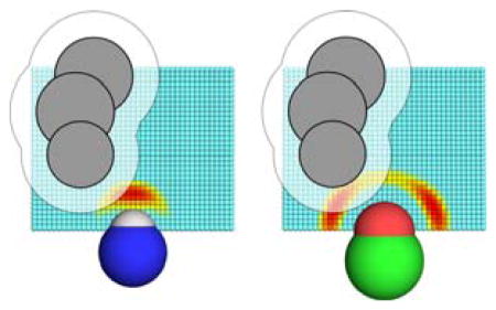
The SHO (“Solvent Hydrogen bond Occlusion”) approach assigns desolvation free energies for individual polar groups, by evaluating the extent to which neighboring atoms prevent the polar group from engaging in hydrogen bonds with solvent. A single probe water molecule is considered, which can occupy grid points around the polar group of interest; the energetics on the grid reflect the preferred hydrogen bonding geometry for the polar atom of interest (color gradient). Neighboring atoms (shown in grey) sterically occlude the probe water from certain locations on the grid: by writing a partition function that sums over these grid points, we can explicitly evaluate the desolvation free energy due to these occluding atoms.

Introduction

Interactions with solvent represent a key contribution to the energetics that determine biomolecular structure, and in turn their function. These interactions are often described by the sum of two effects [1]. The first involves penalizing exposed hydrophobic groups of the biomolecule, due to the entropic cost of ordering solvent around these groups [2,3]. The second entails penalizing buried polar groups in the protein interior, since burial of these groups comes at the expense of favorable interactions with solvent [4].

It is well established that introducing into a protein an “unsatisfied” polar group—a group sequestered away from solvent but not forming a compensatory hydrogen bond to solute—is highly destabilizing [5–8]. Fleming and Rose [9] estimated an energetic cost of ~5 kcal/mol for loss of a hydrogen bond to solvent, and on this basis pointed out the extreme unlikelihood of finding such features in protein structures. They further examined in detail a number of examples identified in a previous survey of crystal structures [10], and found that most occurred in regions of poor crystallographic density and/or could be resolved by selection of a different side-chain rotamer [9].

In this study, we begin from the observation that burial of polar groups is not necessarily modeled accurately by standard modern continuum approaches. This insight spurs us to propose the first model of biomolecular solvation, SHO (“solvent hydrogen-bond occlusion”), that seeks to capture specific polar first-shell interactions without adding additional (solvent) particles to the simulation. As with other implicit solvent models, SHO takes into account both enthalpic and entropic effects of desolvation: thus, it aims to report on desolvation free energies, rather than energies.

Historically, new models for calculating energetics of solute–solvent interactions have often been benchmarked on their ability to recapitulate hydration free energies (gas-to-water transfer free energies). The value of such studies, and the interest in improving the underlying computational methods, has motivated organization of recurring “SAMPL challenges” as blind tests of various methods’ ability to predict hydration free energies [11]. While the intention of SHO is to accurately capture the effect of polar desolvation, a number of other important factors also contribute to hydration free energies (including non-polar solvation, conformational entropy, and parameters for atypical functional groups) that may obscure the performance of SHO in capturing this particular element of biomolecular solvation.

For this reason, we instead turn to a more pragmatic and focused series of benchmarks: we will directly evaluate the performance of SHO in the context of realistic protein structure prediction and virtual screening tasks. These comparisons will take place using the Rosetta macromolecular modeling software [12]; accordingly, in these studies we explore the effect of replacing Rosetta’s default treatment of polar solvation, that of EEF1 [13], with SHO. We note that the simulation community frequently makes use of more advanced theoretical frameworks for continuum treatment of bulk solvent, most notably numerical solutions of the Poisson–Boltzmann equation (PB) or an approximation to it, the Generalized Born model (GB) [14–16]. Because it is non-trivial to effectively “mix and match” pieces of a complete energy function without careful re-parameterization, we will restrict the present study to a comparison of the performance of SHO versus that of EEF1 in the context of Rosetta’s default energy function; a thorough comparison of multiple models for polar solvation will be reported separately.

The SHO model

Our SHO (“Solvent Hydrogen bond Occlusion”) approach seeks to assign desolvation free energies for individual polar groups, by evaluating the extent to which neighboring atoms prevent the polar group from engaging in hydrogen bonds with the solvent. Because our initial evaluation of SHO takes place using the Rosetta energy function, this first implementation is built upon the Rosetta hydrogen bond term.

Hydrogen bond energies in Rosetta are computed as a function of four degrees of freedom that define the geometry of the interacting atoms: δ, Θ, Ψ, and X (Figure 1A). Originally, energies were defined under a purely knowledge-based approach, using the relative frequency at which the current values of these parameters (δ_i, Θ_i, Ψ_i, and X_i) occurred in the Protein Data Bank (PDB) as follows [17,18]:

$$E_{hb}^i\propto min(-k_{B}T\left(ln\left(\frac{P(\delta ={\delta }_i)}{P_{\mathit{ref},\delta }}\right)+ln\left(\frac{P(\mathrm{\Theta }={\mathrm{\Theta }}_i)}{P_{\mathit{ref},\mathrm{\Theta }}}\right)+ln\left(\frac{P(\mathrm{\Psi }={\mathrm{\Psi }}_i)}{P_{\mathit{ref},\mathrm{\Psi }}}\right)+ln\left(\frac{P(\mathrm{X}={\mathrm{X}}_i)}{P_{\mathit{ref},\mathrm{X}}}\right)\right),0)$$ (1)

Figure 1. The SHO model for polar solvation.

A) The geometry-dependence of hydrogen bonding, as exemplified through the degrees of freedom used by the hydrogen bond term in Rosetta energy function. The distance δ and the angles Θ, Ψ and X are defined with respect to the acceptor atom “A”, the hydrogen bond donor “H”, and the atoms to which each of these are connected “AB” and “DB”. B) For SHO calculations, a cubic grid is built around the polar group of interest: a probe water molecule can occupy any of these points, or else one of many degenerate locations in bulk solvent (not shown). Grid points are colored based on the hydrogen bond energy of a probe water molecule placed at that location (expressed in Rosetta Energy Units, REUs); the energetics captured on the grid thus reflect the preferred hydrogen bonding geometry for the polar atom of interest, as shown for this donor (left) and acceptor (right). Neighboring atoms (grey) sterically occlude the probe water from certain locations; these points correspond to those covered by the atoms themselves, and also to the regions too close to these atoms to be accessible to the probe water (grid points covered by the transparent area). By summing over these occluded locations, we explicitly evaluate the desolvation free energy as described in Equation 5.

The Rosetta hydrogen bond term has since been elaborated through the use of a smoothing function, and by re-fitting the terms in the parametric functional form of this equation to remove double-counting with other terms in the energy function and empirically recapitulate the hydrogen bond geometries observed in the PDB [19]. Nonetheless, we note that the SHO approach can, in principle, be built upon any functional form that yields hydrogen bond energies, and is not necessarily tied to that of Rosetta’s energy function.

To evaluate the polar desolvation free energy of a given polar group, the SHO approach begins by considering a single probe water molecule, and discretizing its position variables: the water may occupy one of N positions near the polar group, or else one of g (degenerate) locations in bulk solvent (Figure 1B). If the probe water is located near the polar group, it is assumed to be optimally oriented for hydrogen bonding and its energy is then obtained using Rosetta’s hydrogen bond term. If the probe water instead occupies any of the g locations in bulk solvent, it instead has energy E_bulk.

We can write down the partition function of this system by summing over all states that can be occupied by the water molecule (with β = 1/k_BT):

$$Z_{\mathit{tot}}=Z_{\mathit{bulk}}+Z_{\mathit{grid}}=g{e}^{-\beta E_{\mathit{bulk}}}+\sum _{i=1}^N{e}^{-\beta E_{hb}^i}$$ (2)

Given this partition function, the probability that the probe water occupies a specific location i near the polar group can then be written as:

$$P(\mathit{probe}\mathit{water}isati)=\frac{e^{-\beta E_{hb}^i}}{Z_{\mathit{tot}}}$$ (3)

The presence of one or more “occluding” atoms near the polar group can exclude the probe water from certain locations, due to steric overlap (Figure 1B). Using the same complete partition function, we can then calculate the probability that the water molecule is not displaced by the occluding atom(s) by:

$$P(\mathit{solv})=\frac{Z_{\mathit{bulk}}+{\sum }_i^{\mathit{allowed}\mathit{grid}\mathit{points}}{e}^{-\beta E_{hb}^i}}{Z_{\mathit{tot}}}=1-\frac{{\sum }_i^{\mathit{occluded}\mathit{grid}\mathit{points}}{e}^{-\beta E_{hb}^i}}{Z_{\mathit{tot}}}$$ (4)

By analogy to cavitation free energies computed from probabilities of observing the corresponding empty cavity in a simulation of water [20], we can calculate the energetic cost of water vacating the occluded region, E_SHO, from the probability that the water molecule was not occupying any of these particular sites:

$$E_{\mathit{SHO}}=-\frac{1}{\beta }ln(P_{\mathit{solv}})=-\frac{1}{\beta }ln\left(1-\frac{{\sum }_i^{\mathit{occluded}\mathit{grid}\mathit{points}}{e}^{-\beta E_{hb}^i}}{Z_{\mathit{tot}}}\right)$$ (5)

We note that this expression implicitly integrates over the probe water’s rotational entropy, by assuming that water near the polar group is optimally oriented for hydrogen bonding: as noted earlier, E_SHO is therefore not strictly an energy, but rather a free energy. Using this expression, the value of E_SHO for a polar group is zero when it is completely exposed (i.e., none of the locations near the polar group are occluded). When the polar group is completely buried (i.e., all of the locations near the polar group are occluded), the value of E_SHO is a constant that depends on Z_bulk. To match the thermodynamic measurements [21] used in the parameterization of EEF1 [13], and in keeping with other previous estimates [9,22], we set Z_bulk such that complete burial of a polar group would come at an energetic cost of 5 kcal/mol: this is the sole adjustable parameter in our model.

There are a number of inherent over-simplifications in this initial SHO model; these will be considered extensively in the Discussion section. In the sections below, meanwhile, we will describe practical aspects of its implementation and the characterization of its performance.

Evaluating SHO energies in Rosetta

Our original implementation of SHO is included in the Rosetta software suite [12]. The standard hydrogen bond term in the Rosetta energy function divides polar groups into hydrogen bond acceptors and donors (Figure 1A), where acceptors are heavy atoms (in proteins, these are either oxygen or nitrogen) and donors are hydrogen atoms (in proteins, these are attached to either oxygen or nitrogen atoms): there are currently 20 acceptor types and 13 donor types in Rosetta. Given that our implementation of SHO is built upon Rosetta’s hydrogen bond term, we use the corresponding sets of group types for evaluating E_SHO.

Sites around the polar group of interest that may be occupied by the probe water are generated using a cubic grid (Figure 1B). The origin is defined at the position of the polar group’s outer atom, and the z-axis is defined as the direction of the “base” atom to which it is attached. The grid spans the [−5 Å, +5 Å] range along the x- and y-axes, and the [0.25 Å, 8.25 Å] range along the z-axis; at z ≤ 0 water cannot form a hydrogen bond with the polar group. The grid spacing is set to 0.25 Å along all three axes, resulting in 55,473 total grid points; using finer grid spacing was found not to affect calculated values of E_SHO.

At runtime initialization of Rosetta, a representative grid is built for each polar type around a fictitious group of that type. A water molecule is placed in turn at each point of the grid to evaluate hydrogen bonding to the polar group, as per the Rosetta energy function: this implicitly captures the orientation dependence of hydrogen bonding in protein structures and quantum mechanical calculations [17–19]. This underlying geometric dependence is easily observed in the preferred water locations near a hydroxyl acceptor, which are aligned with the lone pairs of this sp³ hybridized acceptor atom (Figure 1B) rather than in line with the C–O bond. As the water probe is moved from point to point, the corresponding $e^{-\beta E_{hb}^i}$ values are pre-computed and stored in memory. Given the sum over all $e^{-\beta E_{hb}^i}$ values, the value of Z_tot is calculated such that a completely occluded polar group will give an E_SHO value of 5 kcal/mol (per Equation 5): setting Z_tot in this manner is equivalent to indirectly adjusting the value of Z_bulk to achieve the same effect, and ensures that these values are automatically updated even if the grid spacing or hydrogen bond term changes.

To evaluate E_SHO for an actual polar group in the macromolecule, the polar group and its neighboring atoms (atoms belonging to residues within 10 Å of the polar group’s residue) are mapped to the appropriate pre-built grid. All grid points around the polar group are initially marked as “available” to the probe water. For each neighbor atom, grid points at which the neighbor atom would collide with the water molecule—i.e., points whose distance to the neighbor atom is lower than the summed radii of the neighbor atom and of the water molecule—are then marked as “occluded”. By default, we only consider occlusion of the polar group by non-hydrogen atoms: we found including hydrogens had a negligible effect on the resulting E_SHO values. After all neighbor atoms have been considered, the $e^{-\beta E_{hb}^i}$ values for occluded positions and the Z_tot value are retrieved from memory, and used to calculate E_SHO as described in Equation 5.

Incorporating SHO into the Rosetta energy function

The Rosetta energy function is comprised of a linear combination of terms, each designed to capture a separate physical force: these terms are carefully weighted with respect to one another, for performance in a wide variety of modeling tasks. Solvation is captured implicitly via the EEF1 solvent model [13], which can be broken into two parts: one favoring burial of non-polar groups, and the other penalizing burial of polar groups. Since SHO seeks only to model the latter part (polar desolvation), for incorporation of SHO into Rosetta we retained the non-polar part of EEF1, and replaced the polar part of EEF1 with SHO.

Further, the hydrogen bond term in Rosetta is also built with the expectation that its functional form will be applied in conjunction with EEF1: the different geometry-dependence of SHO is likely to require recalibration of this term. In particular, SHO most disfavors positioning of non-bonded atoms at locations optimal for hydrogen bonding to a polar group, whereas EEF1 free energies depend primarily on distance and are mostly agnostic to further details of geometry. Thus, SHO is expected to flatten the energetic dependence on geometry that is currently encoded in Rosetta’s hydrogen bond term, if simply used as a replacement for EEF1.

Rather than alter Rosetta’s hydrogen bond term and re-fit each of the weights that balance the energy function, for the purposes of this study we sought to incorporate SHO in a minimally disruptive fashion. Thus, we elected to continue treating polar groups hydrogen-bonded to other solute groups using EEF1: only polar groups that are not hydrogen-bonded to other solute groups are treated using SHO.

In order to match the free energy scale of SHO values to the EEF1 values which they replace, we used both models to evaluate the desolvation free energy of 61,476 non-hydrogen-bonded polar groups from 207 crystal structures with resolution of 1.0–1.5 Å of non-redundant proteins (this dataset is described in further detail in the Results section). Since the EEF1 model defines free energies for individual heavy (non-hydrogen) atoms rather than for polar groups [13], we split the EEF1 energy amongst each of the hydrogen bond donors/acceptors on a given atom (e.g. the EEF1 energy for lysine Nζ was divided equally amongst its three protons). We found the SHO and EEF1 average free energies over this set of polar groups to be related by a proportionality constant of 0.4775. By applying this proportionality constant to the free energies computed by SHO, we match the internal free energy scale used by Rosetta’s implementation of EEF1.

Results

Buried unsatisfied polar groups in the PDB

As a consequence of the energetic importance of hydrogen bonding, it is expected that very few polar groups in protein structures will be “unsatisfied” [9]. Rather, with few exceptions, a protein’s polar groups will either engage in hydrogen bonds to other solute atoms (particularly intramolecular hydrogen bonds that comprise protein secondary structural elements) or else will form hydrogen bonds to solvent. As noted earlier, the free energy cost of a truly “unsatisfied” polar group is expected to be large, such that these should not often be observed in crystal structures of proteins [9,10].

Using SHO, we can directly examine the frequency with which polar groups not hydrogen bonded to solute are indeed available for hydrogen bonding to solvent. We began by generating non-redundant sets of protein structures binned by crystallographic resolution, using the PISCES server [23] (see Methods section). Among polar groups not engaged in intramolecular hydrogen bonds, based on the distribution of E_SHO values (Figure 2A) we defined any polar groups with E_SHO > 4.9 kcal/mol as “unsatisfied” (SHO was set up with a maximum possible value of 5.0 kcal/mol). The underlying SHO calculation explicitly places a water probe molecule at sites around the polar group of interest; here, we are essentially re-using this calculation to identify polar groups around which no water molecule can be placed without steric interference from neighboring atoms.

Figure 2. SHO disfavors buried unsatisfied polar groups.

A) The distribution of E_SHO values is collected from 207 protein structures with crystallographic resolution 1.0–1.5 Å, for a total of 61,476 polar groups not participating in hydrogen bonds within the solute. Z_tot (defined in Equation 2) was set such that the maximum possible value of E_SHO would be 5.0 kcal/mol. B) The percentage of polar groups that are not hydrogen bonded to other solute atoms and not “satisfied” by solvent (E_SHO > 4.9 kcal/mol) is reported as a function of crystallographic resolution. Higher resolution structures are found to have fewer unsatisfied polar groups. Because most polar groups that meet this criterion are completely desolvated (as seen in panel A), these results are not sensitive to the precise value of E_SHO used as cutoff for defining “unsatisfied” groups. C) Drawing only from polar groups that are not hydrogen bonded to other solute atoms, the polar solvation free energy was calculated using SHO and EEF1. While the average polar solvation free energy from SHO increases dramatically at poor resolution, this trend is not observed for EEF1. In both cases, the polar solvation free energies are expressed in Rosetta Energy Units (REUs).

For all of the polar groups in each resolution bin, we evaluated the overall percentage that were “unsatisfied” by this definition (Figure 2B). From this analysis we find that highest-resolution crystal structures, in which the modeled atomic coordinates are most constrained by the electron density, contain the fewest buried unsatisfied polar groups. In contrast, protein structures solved at poorer resolution—where the refinement force field contributes more to the final coordinates—have many more unsatisfied polar groups: this implies that modern methods for crystallographic refinement do not adequately focus on avoiding these unfavorable structural features. This trend has also been observed previously using a much smaller dataset, albeit using a simpler strategy that is prone to false positives when evaluating whether a given polar group can form a hydrogen bond to solvent [10].

Given that protein structures solved at poorer resolution have more unsatisfied polar groups, one would expect that their polar solvation free energy should be higher: indeed, this is precisely the physical phenomenon that this free energy term seeks to capture. This trend, however, is not convincingly captured by the EEF1 model of polar solvation, at least as implemented in Rosetta (Figure 2C): among polar groups not engaged in hydrogen bonds to other solute atoms, the average polar solvation energy for these groups is nearly flat for all but the lowest-resolution structures. On the other hand, the average SHO free energy of the same non-hydrogen-bonded polar groups exhibits a consistent increase with decreasing resolution. In some ways this is unsurprising, as we have already shown that SHO detects more unsatisfied polar groups using a definition directly built on E_SHO itself. Nonetheless, the stark contrast in behavior between EEF1 and SHO in this experiment highlights the substantive difference in how these two models penalize burial of polar groups.

Discrimination of native-like protein loops

The effects of polar solvation are particularly important at partially-buried regions of protein structure [24]; this makes loop modeling an ideal high-resolution context in which to test SHO. A recent “robotics-inspired” loop-modeling approach named NGK [25,26] has enabled vast enhancements in conformational sampling of loop regions in proteins. While this improved sampling led to tremendously accurate predictions in several cases, it also served to highlight the difficulty in identifying the best output model (i.e., the model closest to the crystallographic, or “native”, loop conformation) from among all the models generated. Typically, one selects the model for which the total energy of the protein is lowest as the final predicted structure. Given the extensive sampling provided by NGK, we used this method to build a set of output models and then asked whether replacing EEF1 with SHO would impact the final predicted structures.

For this study we chose a standard benchmark set of 45 12-residue loops, that was previously used to test the NGK sampling protocol [27,28]. For each target loop we first generated a set of 500 NGK models using the standard Rosetta energy function (which includes EEF1 as the solvation term). NGK models could not be generated using SHO at this point, because the functional form of SHO is currently incompatible with NGK’s gradient-based minimization algorithm. We then scored each model either using the default Rosetta energy function, or having replaced the polar part of EEF1 with SHO. We emphasize that with the exception of the polar solvation term, the energy function for the two scoring methods was identical.

Figure 3 shows the RMSD to the native loop of the lowest-energy loop model obtained using either EEF1 or SHO to capture polar solvation. For 24 of the 45 targets the two scoring methods performed essentially the same, i.e., selecting models within 10% RMSD of one another, and often the same specific model. For these targets other energetic contributions dominate, and thus polar solvation is not the main determinant responsible for success or failure in identifying a native-like model. Among the other 21 targets, meanwhile, we find that in 14 cases the lowest-energy model identified by SHO is closer to the crystal structure than the lowest-energy model identified by EEF1.

Figure 3. Applying SHO for loop modeling discrimination.

For each of 45 target loops, 500 models were generated and then the lowest−energy model was selected using the Rosetta energy function with EEF1 or using the Rosetta energy function with SHO. The RMSD of the loop region was calculated for the model selected by each method. Each point on the plot represents a different target loop; points below the diagonal represent targets for which SHO led to selection of a more “native-like” model than EEF1. Excluding “ties” (cases in which the RMSDs for both methods were within 10% of one another), SHO outperforms EEF1 for 14 targets whereas EEF1 outperforms SHO for 7 targets.

The difference in performance between SHO and EEF1 is not quite statistically significant (p=0.14, per the one-tailed Wilcoxon signed-rank test), because of the relatively small number of targets in this benchmark set; nonetheless, this result suggests that simply replacing EEF1 with SHO for scoring protein structures may prove advantageous in loop modeling applications.

We must note, however, that the models themselves were generated using EEF1, which may slightly disadvantage EEF1 in this comparison (the “decoy” models generated are specifically those that correspond to minima on the EEF1 energy landscape). Since this initial implementation of SHO is currently not suitable for carrying out extensive conformational sampling, we will defer a fully “fair” comparison in this regard to our upcoming model that allows such sampling by approximating SHO free energies using a simpler functional form [29].

Virtual screening for small-molecule inhibitors of protein–protein interactions

We previously showed that small-molecule inhibitors of protein–protein interactions (PPIs) bind to shallower pockets than inhibitors of more traditional drug targets, such as enzymes and G protein-coupled receptors [30]. Given that the inhibitors in the former case remain quite exposed to solvent when bound to their protein partners, we surmised that here too a more accurate modeling of polar solvation might help discriminate native-like models. As a pragmatic application, we therefore sought to explore the effect of replacing EEF1 with SHO for distinguishing active versus inactive compounds when docked to a protein of interest; this is precisely the task that one carries out in the final step of virtual screening, and is a problem that is still very challenging for PPI inhibitors [31].

For this experiment we chose to use our previously-described benchmark set that includes 18 diverse proteins for which a crystal/NMR structure is available in complex with a small-molecule PPI inhibitor [31]. In our previous studies we had built a non-redundant set of 2500 “decoy” compounds, and docked each of these to the PPI binding pocket [31]; the virtual screening task then consists of identifying the sole active compound that has been hidden among these decoy compounds. To do so, each of the complexes for a given target is scored, and ranked on the basis of protein–ligand interaction energy as calculated by Rosetta. Success in this experiment involves ranking the known active compound ahead of as many decoys as possible. We note that the active compound is used in the native pose, rather than itself being docked. This simplification focuses the benchmark fully on the discrimination step: using instead the re-docked native poses would have added noise, since mis-docked inhibitors should not be considered “correct” for a given target at the scoring stage we consider here [31]. Also, we note that the use of multiple protein targets entails a distinct active compound for each complex (Figure S1), thereby avoiding potential bias associated with a benchmark that focuses on a single protein and/or ligand.

We scored each model complex and evaluated the interaction energy either using the default Rosetta energy function, or having replaced the polar part of EEF1 with SHO (Figure 4A). For 6 targets, the rank of the known inhibitor was equivalent with either method, to within 10% (“ties”)—these include 4 cases for which the known inhibitor ranks first overall, ahead of every decoy compound. Among the other 12 targets, we find that in 7 cases SHO assigns a better ranking to the known active compound, and in the other 5 cases EEF1 assigns a better ranking. In many of these cases, the “margin of victory” for targets won by SHO is larger than for targets won by EEF1; while the overall difference in performance between the methods is again not statistically significant due to the relatively small number of targets, the large impact of using SHO for certain targets is reflected in the p-value computed via the one-tailed Wilcoxon signed-rank test (p=0.16).

Figure 4. Applying SHO to identify small-molecule inhibitors of protein–protein interactions.

For each of 18 target proteins, 2500 “decoy” compounds were docked to the protein interaction site; the energies of these decoys were compared to that of a known “active” compound for each complex (the active compound differed for each target protein, the complete collection is shown in Figure S1). For each of these complexes and their corresponding native complex, the interaction energy was determined using the Rosetta energy function with EEF1 or using the Rosetta energy function with SHO. For each target, we report the rank of the active compound (i.e., the native complex) relative to the decoys; each point on the plots represents a different protein target. Points below the diagonal represent targets for which SHO ranked the active compound ahead of more decoy compounds than EEF1. A) In the initial benchmark, the protein–ligand complexes were not pre-minimized. Excluding “ties” (cases in which the ranks for both methods were within 10% of one another), SHO outperforms EEF1 for 7 targets whereas EEF1 outperforms SHO for 5 targets. Only 6 points are visible for the former, because there are two targets for which the rank by SHO is 1 and the rank by EEF1 is 2. B) In the subsequent experiment, each of the protein–ligand complexes was pre-minimized using the standard Rosetta energy function. In this more challenging benchmark, SHO outperforms EEF1 for 11 targets whereas EEF1 outperforms SHO for 5 targets.

As we noted in our previous studies involving this benchmark [31], some of the docked decoy complexes include steric clashes that can be easily identified by Rosetta. We therefore surmised that the ability to discard many decoys on the basis of sterics alone might have partly obscured some underlying differences in performance between SHO and EEF1. To make the virtual screening task more challenging, we therefore considered the same protein–ligand complexes after they had undergone energy minimization to resolve steric clashes, using the standard Rosetta energy function (i.e., using EEF1) [31]. We then rescored the minimized complexes (both native and decoy), using either EEF1 or SHO to model polar solvation.

The overall performance in this new regime became much worse regardless of which method was used to model polar solvation, underscoring the fact that this is truly a challenging benchmark (Figure 4B). Nonetheless, of the 16 targets that are not “ties”, there are 11 in which SHO outperforms EEF1 (whereas EEF1 outperforms SHO for the other 5 targets). The one-tailed Wilcoxon signed-rank test also recognizes this difference, albeit not quite at a statistically significant level due to the size of our benchmark set (p=0.065).

The paucity of examples in the PDB to draw from makes it impossible to expand our test set [32,33], and perhaps obtain results at statistical significance. However, the observations presented here nonetheless suggest that SHO’s treatment of polar solvation may allow for improved results in virtual screening for inhibitors acting at protein interaction sites. That said, the overall poor performance in the second benchmark clearly points to the need for improvements in the Rosetta energy function, presumably beyond simply the treatment of polar solvation.

Discrimination of native-like protein structures

The CASP11 protein structure prediction experiment in 2014 included a refinement challenge: here, 53 groups competed by submitting their best state-of-the-art structural predictions for 37 different protein targets, starting from protein structures predicted by a server. The competitors each used their own preferred methodologies, which vary significantly from one another. Nonetheless, collectively they represent cutting-edge modern approaches for molecular modeling, and overall many of the models were improved relative to the starting structure (i.e., closer to the native structure) [34].

At the outset of our studies, we demonstrated that SHO energetically distinguishes between high- and low-resolution crystal structures, by penalizing buried unsatisfied polar groups (Figure 2). In light of SHO’s ability to detect these subtle structural details, we anticipated that SHO might also distinguish between native protein structures and the near-native models produced in the refinement portion of CASP11. For each of the 36 CASP11 targets whose native structure is available in the PDB, we therefore used both EEF1 and SHO to evaluate the average solvation free energy for non-hydrogen-bonded polar groups, both in the native structure and in the models provided by CASP participants. Among the models, we considered only “model-1” from each submitter: the model that they themselves considered to be their best model.

Using EEF1, the native structure had lower polar solvation free energy than the average of the models for 21 of 36 protein targets; for the other 15 targets, the models had lower average free energy than the native structure (Figure 5A). While the methods used in building the models differ from group to group, overall the inability of EEF1 to distinguish between the models and the native structure implies a correlation between EEF1 free energies and the energy functions used by these various groups in building their models.

Figure 5. Applying SHO to identify native protein structures.

For each of 36 CASP11 refinement targets, quantities measured for the native structure are compared to those averaged over the “model-1” submissions from each participant. A) The average EEF1 free energy for polar groups not engaged in hydrogen bonds is lower for the native than for the average of the models in 21 of 36 cases (points below the diagonal); in the other 15 cases, the average of the models is lower than the native. B) Using SHO, the average free energy for the same set of polar groups is lower for the native structure in all 36 targets (points below the diagonal). Thus, SHO provides energetic discrimination for native versus near-native protein structures. C) Using SHO to identify buried unsatisfied polar groups, we find that these unfavorable features occur more frequently in the models than in the corresponding native structures (all points are below the diagonal): this provides the basis by which SHO discriminates energetically between native and near-native structures.

In contrast, the polar solvation free energy from SHO for the same set of polar groups was lower for the native than for the models in every one of the 36 targets included in this set (Figure 5B). This observation strongly implies that SHO detects, and penalizes, structural features in the models that are insufficiently penalized by the modern methods used to generate these models. Naturally, we expect that these “structural features” are buried unsatisfied polar groups; we therefore used the SHO-derived criteria described earlier to count the frequency of buried unsatisfied polar groups in the native proteins and in the models (Figure 5C), and confirmed that in every case, the models on average contain more buried unsatisfied polar groups than the corresponding native protein. We therefore conclude that appropriate penalization of buried unsatisfied polar groups is crucial to SHO’s ability to energetically distinguish between native and near-native protein structures—and that this is a key element missing from at least most of the modern energy functions used in this CASP11 challenge.

Discussion

Comparison with other models of polar solvation

Interactions with solvent are critical to biomolecular structure and function, but explicitly including an appropriate number of solvent molecules would make many applications intractable. Modern implicit solvation models employ a continuum treatment of solvent, and are thus built to capture long-range energetic effects but focus less on interactions in the first solvation shell. Accordingly then, this continuum treatment of solvent may not accurately model energetic contributions that arise from hydrogen bonding between a biomolecule and the specific discrete water molecules around it, particularly at partially exposed regions of the biomolecule.

Here we report our initial development of SHO, a model of polar desolvation built to explicitly consider whether the geometry of nearby occluding groups precludes hydrogen bonding to solvent. Because interactions with specific solvent molecules in the first solvation shell are so important, two classes of models have been developed to directly address these interactions. The first are “hybrid” models, which add a layer of explicit water molecules (either to the active site or the whole macromolecule), while representing additional interactions through a continuum model. These water molecules can either be free to move during the simulation [35,36], or, in the First-Shell Hydration (FiSH) model, be confined to the solvent-accessible surface of the solute [37]. The second class of model involves adding a series of dipoles (representing water) that are confined to a grid around the biomolecule but are free to change their orientation in response to the conformation of the biomolecule [38–40]. Both of these classes of models have the disadvantage that they increase the number of particles in the system, and therefore come with computational expense greater than that of traditional implicit solvation models.

The closest analogous model to SHO, in its philosophy, is the recent Semi-Explicit Assembly (SEA) water model [41]. Here, the authors pre-computed the water distribution around several different “atomic” solute spheres from explicit solvent simulations. To evaluate the solvation free energy of an arbitrary molecule, they then assemble together the solvation responses from the appropriate component spheres. While the SEA approach recapitulates certain phenomena that are not captured by traditional continuum implicit solvent models (e.g., the “charge asymmetry” of water’s dipole around positively versus negatively charged solutes), to date this model has been exclusively deployed for predicting solvation free energies of small molecules [42,43]; thus, it is unclear the extent to which SEA will offer improved accuracy for simulations involving macromolecules.

The SHO approach is also similar in spirit to studies in which explicit-solvent molecular dynamics simulations were used to estimate the probability that any particular polar group is solvated [44–48]. The reliance of each of these methods on such a simulation, however, makes evaluation of solvation free energies very costly and limits their applicability to specific cases.

Current limitations of SHO

The present formulation of the SHO model makes several key assumptions, most stemming from our use of Rosetta hydrogen bonding energies as the basis for determining the importance of each grid point (Figure 1). While convenient, this simple strategy requires that only a single water probe molecule is treated at any given time. Because of this, we neglect the fact that one water molecule may prevent other water molecules from simultaneously approaching the polar group or, alternatively, may form favorable interactions with other water molecules. The latter have recently been observed in molecular dynamics simulations as playing a particularly important role in folding of β-strands, through a mechanism in which formation of each inter-strand hydrogen bond is coupled to the formation of a hydrogen bond between two water molecules (besides the loss of two strand–water-molecule hydrogen bonds) [49]. Beyond first-shell water–water interactions, the present formulation also neglects the contribution of second-shell (and higher order) water molecules. In addition to these limitations, our current model also evaluates the interactions of this water molecule only in relation to a single polar group: this neglects the fact that the rest of the environment itself contributes to the energetics of placing a water molecule at a particular location, as waters that “bridge” multiple solute polar groups may be especially favorable, and may also play a particularly important role in protein folding [50].

Finally, our model assumes that the probe water molecule is optimally oriented with respect to the polar group of interest, and uses Rosetta’s knowledge-based hydrogen bond parameters derived from crystal structures; the appropriateness of both of these assumptions is unclear for water near a protein surface at physiological temperature. These latter assumptions, at least, derive from our decision to assign energies to grid points using Rosetta’s hydrogen bond potential. One could very naturally instead obtain analogous information either from experimental water residence times [51,52], or by explicitly collecting occupancy statistics from explicit-solvent molecular dynamics simulations of suitable small model compounds.

It will be interesting to determine, through future studies, whether improvements in the accuracy of these underlying grid energetics, based on subtle redistribution of occupancy probabilities to address all of the neglected contributions described above, can lead to tangible improvements in the overall performance of SHO.

Extending beyond SHO

In its current form, potential applications of SHO are limited to those which can be carried out entirely through scoring static structures, rather than for conformational sampling. The formulation of SHO presented in Equation 5 is not smoothly differentiable with respect to atomic coordinates, because the summation over grid points depends in a discrete way on whether or not a given point is occluded. While it could in principle be used for Monte Carlo simulations, these are much more efficient if each energy term can be broken into a sum of pairwise atomic (or residue) contributions; our present formulation of SHO is not pairwise additive in this manner either. Finally, even for stand-alone energy evaluations our current implementation of SHO is 2 to 7 times slower than the Rosetta EEF1 implementation for typical protein sizes (i.e., 50–450 residues), with the gap widening as the size of the protein increases.

To address these clear limitations, we have recently fit free energies derived from SHO to a simple functional form that is analytically differentiable, pairwise-additive, and very fast (comparable in speed to EEF1) [29]. In essence, our strategy mimics that of others who have built simple implicit models by matching to explicit-solvent solvation forces [53]: the objective of our development of “pwSHO” was to recapitulate the geometry-dependence encoded in SHO through a model that can replace EEF1 for all conformational sampling—both in Rosetta and in other energy functions. By including SHO polar desolvation in conformational sampling, rather than simply in post hoc re-scoring of static structures, it will be possible to study more directly the role played by buried unsatisfied polar groups in phenomena such as protein folding and protein–protein association that depend critically upon the balance of hydrogen bonding and hydrophobic interactions [50].

We note that SHO is highly sensitive to precise conformational details: subtle rearrangements can have drastic energetic consequences, as an unsatisfied polar group can adjust very slightly and form a hydrogen bond to solvent that was previously not possible. Indeed, this sensitivity underlies SHO’s ability to distinguish high- versus low-resolution crystal structures, and native versus near-native protein structures. On the other hand, the same sensitivity can be detrimental when SHO is applied only for scoring: if the most native-like available structure has slight deficiencies corresponding to buried unsatisfied polar groups, the structure may be strongly penalized by SHO. For this reason, we anticipate that the performance of SHO may be further improved in benchmarks for which the native structure itself is not available (e.g., Figure 3, Figure 4b), if all conformations are first pre-minimized with pwSHO. Indeed, already we have found that incorporating a pre-minimization step with pwSHO, as opposed to EEF1, into the PPI virtual screening benchmark presented here led to significantly improved discrimination of active compounds [31].

Outlook

The key to the improved discrimination of native protein structures afforded by SHO appears to derive primarily from its ability to identify models with fewer buried unsatisfied polar groups. To a first approximation, at least, this appears to be a powerful means to separate models that are truly correct from models that are simply “near-native”; compelling support for this argument comes from SHO’s ability to distinguish high- versus low-resolution crystal structures. Our results suggest that simple avoidance of buried unsatisfied polar groups may provide an avenue towards dramatic improvements in high-resolution structure prediction; the same results also underscore the fact that these unfavorable structural features are insufficiently penalized by most modern treatments of polar solvation.

We anticipate that the largest benefit from improved descriptions of polar solvation will come specifically at surface loops and interfacial regions in biomolecules that constitute binding sites for proteins and small-molecules: exactly those elements of structure which are most important for understanding and manipulating function. Particularly with the advent of cryo-electron microscopy (cryo-EM) for obtaining structures at near-atomic (~3.3 Å) resolution and even beyond [54,55], there is increased need for ultra-high-resolution molecular modeling to help explain the basis for phenomena that rely on precise details of molecular structural variability [56,57].

Methods

The SHO model of polar desolvation is implemented in the Rosetta software suite [12], and can be used in all applications that do not require derivatives of the energy function. To activate SHO in the Rosetta energy function, one can simply add -score:patch occ_Hbond_sol_exact_talaris2014 to the command line. Rosetta is freely available for academic use (www.rosettacommons.org).

Rosetta energy function

For all the experiments described here, we incorporated the SHO and EEF1 polar solvation terms into the current default Rosetta energy function, Talaris2014 [58]. The only exception is the EEF1-based energy minimization of PPI protein–ligand complexes, which was performed using the Talaris2013 energy function as part of our previous study [31].

A proportionality constant of 0.4775 was applied to SHO free energies within Rosetta, in order to match the internal free energy scale of Rosetta’s EEF1 implementation. As described in the section Incorporating SHO into the Rosetta energy function, this value was determined such that EEF1 and SHO desolvation free energies were the same, on average, over non-hydrogen-bonded polar groups in crystal structures solved at 1.0–1.5 Å resolution (Figure 2C).

Non-redundant subsets of the PDB

We built five subsets of crystal structures from the PDB at different resolutions, using the PISCES server [23]. We imposed a sequence identity cutoff of 25% to exclude redundant proteins and required an R-factor of 3.0 or better. The subsets contained a total of 1913 protein chains of 26–200 residues, divided as follows: 207 chains at 1.0–1.5 Å resolution, 635 chains at 1.5–2.0 Å resolution, 595 chains at 2.0–2.5 Å resolution, 352 chains at 2.5–3.0 Å resolution, and 124 chains at 3.0–3.5 Å resolution. All crystal structures were pre-optimized using flags -no_optH false for hydrogen placement and -flip_HNQ true for histidine/asparagine/glutamine flipping.

Rosetta command to identify buried unsatisfied polar groups

Buried unsatisfied polar groups in a given PDB structure were identified using the new shobuns app as follows:

shobuns.linuxgccrelease -s 1agyA.pdb -score:patch occ_Hbond_sol_exact_talaris2014

Loop modeling benchmark

The loop modeling benchmark set, comprised of 45 12-residue loops, is the same set used to previously benchmark the NGK algorithm [26–28]. Before running NGK, to avoid bias from the native environment, the target loop and all side-chains within 10 Å of it were removed from the protein structure. NGK was then applied to produce 500 models per loop, using the following command:

loopmodel.linuxgccrelease -s 1a8d.pdb -loops:loop_file 1a8d.loop
-loops:remodel perturb_kic -loops:refine refine_kic -loops:kic_rama2b
-loops:ramp_fa_rep -loops:ramp_rama -loops:kic_omega_sampling
-loops:allow_omega_move true -ex1 -ex2

PPI virtual screening benchmark

We re-used the benchmark set of 18 unique PPI sites that we had compiled for a previous study, together with all docked models generated at that time [31]. For each protein the decoy set consisted of 2500 ligands of molecular weight between 350 and 550 Da, selected at random from the ZINC database [59] so that no two decoys had a fingerprint Tanimoto score ≥ 0.8, and no decoy had a fingerprint Tanimoto score ≥ 0.5 with respect to the known inhibitor. The first condition was intended to ensure non-redundancy among decoys; the second was to exclude from the decoy set compounds that may themselves be active. Docking was targeted to the known binding pocket, and was carried out by FRED (version 3.0.0) [60–62], which considered up to 300 conformers of each decoy compound as generated by OMEGA (version 2.4.3) [63–65]. Protonation/tautomeric states of decoy ligands were determined using QUACPAC [66]; protonation/tautomeric states of native ligands were determined using Protoss [67] in the context of the target protein (Figure S1). We computed protein–ligand interaction energies in Rosetta as the energy of the protein–ligand complex minus the summed energies of the protein and the ligand taken in isolation. Ligand parameters needed to compute interaction energies were generated by the molfile_to_params python script, which is part of the standard Rosetta distribution.

As in our previous studies [31], we compared the logarithm of ranks (rather than the ranks themselves) when computing p-values, to emphasize the importance of differences at lower-order-of-magnitude ranks.

Native-like protein structure benchmark

The benchmark set consisted of 36 of the 37 protein targets of the CASP11 experiment [34]. Since the native structure of target TR795 was unavailable in the PDB, this target was discarded from the benchmark.

Statistical analysis

We used the one-tailed Wilcoxon signed-rank test (as implemented in the R statistical computing environment [68]) to compute the statistical significance of the improvements we observed in each benchmark. For example, when we considered the improvement of SHO over EEF1 in RMSD between native loop and lowest energy loop model, the R command was the following:

wilcox.test(mydata$eef1_rms, mydata$sho_rms, paired=TRUE, alternative=“greater”)

where $eef1_rms and $sho_rms are the paired lists of RMSD values over the 45 target loops selected using EEF1 and SHO, respectively.

References

- 1.Prabhu N, Sharp K. Protein-solvent interactions. Chem Rev. 2006;106:1616–23. doi: 10.1021/cr040437f. [DOI] [PMC free article] [PubMed] [Google Scholar]
- 2.Kauzmann W. Some factors in the interpretation of protein denaturation. Adv Protein Chem. 1959;14:1–63. doi: 10.1016/s0065-3233(08)60608-7. [DOI] [PubMed] [Google Scholar]
- 3.Soda K. Structural and thermodynamic aspects of the hydrophobic effect. Adv Biophys. 1993;29:1–54. doi: 10.1016/0065-227x(93)90004-o. [DOI] [PubMed] [Google Scholar]
- 4.Tanford C, Kirkwood JG. Theory of Protein Titration Curves. I. General Equations for Impenetrable Spheres. J Am Chem Soc. 1957;79:5333–9. [Google Scholar]
- 5.Blaber M, Lindstrom JD, Gassner N, Xu J, Heinz DW, Matthews BW. Energetic cost and structural consequences of burying a hydroxyl group within the core of a protein determined from Ala-->Ser and Val-->Thr substitutions in T4 lysozyme. Biochemistry. 1993;32:11363–73. doi: 10.1021/bi00093a013. [DOI] [PubMed] [Google Scholar]
- 6.Lim WA, Farruggio DC, Sauer RT. Structural and energetic consequences of disruptive mutations in a protein core. Biochemistry. 1992;31:4324–33. doi: 10.1021/bi00132a025. [DOI] [PubMed] [Google Scholar]
- 7.Loladze VV, Ermolenko DN, Makhatadze GI. Thermodynamic consequences of burial of polar and non-polar amino acid residues in the protein interior. J Mol Biol. 2002;320:343–57. doi: 10.1016/S0022-2836(02)00465-5. [DOI] [PubMed] [Google Scholar]
- 8.Stites WE, Gittis AG, Lattman EE, Shortle D. In a staphylococcal nuclease mutant the side-chain of a lysine replacing valine 66 is fully buried in the hydrophobic core. J Mol Biol. 1991;221:7–14. doi: 10.1016/0022-2836(91)80195-z. [DOI] [PubMed] [Google Scholar]
- 9.Fleming PJ, Rose GD. Do all backbone polar groups in proteins form hydrogen bonds? Protein Sci. 2005;14:1911–7. doi: 10.1110/ps.051454805. [DOI] [PMC free article] [PubMed] [Google Scholar]
- 10.McDonald IK, Thornton JM. Satisfying hydrogen bonding potential in proteins. J Mol Biol. 1994;238:777–93. doi: 10.1006/jmbi.1994.1334. [DOI] [PubMed] [Google Scholar]
- 11.Mobley DL, Wymer KL, Lim NM, Guthrie JP. Blind prediction of solvation free energies from the SAMPL4 challenge. J Comput Aided Mol Des. 2014;28:135–50. doi: 10.1007/s10822-014-9718-2. [DOI] [PMC free article] [PubMed] [Google Scholar]
- 12.Leaver-Fay A, Tyka M, Lewis SM, Lange OF, Thompson J, Jacak R, Kaufman KW, Renfrew PD, Smith CA, Sheffler W, Davis IW, Cooper S, Treuille A, Mandell DJ, Richter F, Ban YE, Fleishman SJ, Corn JE, Kim DE, Lyskov S, Berrondo M, Mentzer S, Popovic Z, Havranek JJ, Karanicolas J, Das R, Meiler J, Kortemme T, Gray JJ, Kuhlman B, Baker D, Bradley P. ROSETTA3: an object-oriented software suite for the simulation and design of macromolecules. Methods Enzymol. 2011;487:545–74. doi: 10.1016/B978-0-12-381270-4.00019-6. [DOI] [PMC free article] [PubMed] [Google Scholar]
- 13.Lazaridis T, Karplus M. Effective energy function for proteins in solution. Proteins. 1999;35:133–52. doi: 10.1002/(sici)1097-0134(19990501)35:2<133::aid-prot1>3.0.co;2-n. [DOI] [PubMed] [Google Scholar]
- 14.Baker NA. Improving implicit solvent simulations: a Poisson-centric view. Curr Opin Struct Biol. 2005;15:137–43. doi: 10.1016/j.sbi.2005.02.001. [DOI] [PubMed] [Google Scholar]
- 15.Koehl P. Electrostatics calculations: latest methodological advances. Curr Opin Struct Biol. 2006;16:142–51. doi: 10.1016/j.sbi.2006.03.001. [DOI] [PubMed] [Google Scholar]
- 16.Decherchi S, Masetti M, Vyalov I, Rocchia W. Implicit solvent methods for free energy estimation. Eur J Med Chem. 2015;91:27–42. doi: 10.1016/j.ejmech.2014.08.064. [DOI] [PMC free article] [PubMed] [Google Scholar]
- 17.Kortemme T, Morozov AV, Baker D. An orientation-dependent hydrogen bonding potential improves prediction of specificity and structure for proteins and protein-protein complexes. J Mol Biol. 2003;326:1239–59. doi: 10.1016/s0022-2836(03)00021-4. [DOI] [PubMed] [Google Scholar]
- 18.Morozov AV, Kortemme T, Tsemekhman K, Baker D. Close agreement between the orientation dependence of hydrogen bonds observed in protein structures and quantum mechanical calculations. Proc Natl Acad Sci U S A. 2004;101:6946–51. doi: 10.1073/pnas.0307578101. [DOI] [PMC free article] [PubMed] [Google Scholar]
- 19.O’Meara MJ, Leaver-Fay A, Tyka MD, Stein A, Houlihan K, DiMaio F, Bradley P, Kortemme T, Baker D, Snoeyink J, Kuhlman B. Combined covalent-electrostatic model of hydrogen bonding improves structure prediction with Rosetta. J Chem Theory Comput. 2015;11:609–22. doi: 10.1021/ct500864r. [DOI] [PMC free article] [PubMed] [Google Scholar]
- 20.Pohorille A, Pratt LR. Cavities in molecular liquids and the theory of hydrophobic solubilities. J Am Chem Soc. 1990;112:5066–74. doi: 10.1021/ja00169a011. [DOI] [PubMed] [Google Scholar]
- 21.Privalov PL, Makhatadze GI. Contribution of hydration to protein folding thermodynamics. II. The entropy and Gibbs energy of hydration. J Mol Biol. 1993;232:660–79. doi: 10.1006/jmbi.1993.1417. [DOI] [PubMed] [Google Scholar]
- 22.Sheu SY, Yang DY, Selzle HL, Schlag EW. Energetics of hydrogen bonds in peptides. Proc Natl Acad Sci U S A. 2003;100:12683–7. doi: 10.1073/pnas.2133366100. [DOI] [PMC free article] [PubMed] [Google Scholar]
- 23.Wang G, Dunbrack RL., Jr PISCES: recent improvements to a PDB sequence culling server. Nucleic Acids Res. 2005;33:W94–8. doi: 10.1093/nar/gki402. [DOI] [PMC free article] [PubMed] [Google Scholar]
- 24.Friesner RA, Abel R, Goldfeld DA, Miller EB, Murrett CS. Computational methods for high resolution prediction and refinement of protein structures. Curr Opin Struct Biol. 2013;23:177–84. doi: 10.1016/j.sbi.2013.01.010. [DOI] [PubMed] [Google Scholar]
- 25.Mandell DJ, Coutsias EA, Kortemme T. Sub-angstrom accuracy in protein loop reconstruction by robotics-inspired conformational sampling. Nat Methods. 2009;6:551–2. doi: 10.1038/nmeth0809-551. [DOI] [PMC free article] [PubMed] [Google Scholar]
- 26.Stein A, Kortemme T. Improvements to Robotics-Inspired Conformational Sampling in Rosetta. Plos One. 2013:8. doi: 10.1371/journal.pone.0063090. [DOI] [PMC free article] [PubMed] [Google Scholar]
- 27.Sellers BD, Zhu K, Zhao S, Friesner RA, Jacobson MP. Toward better refinement of comparative models: Predicting loops in inexact environments. Proteins. 2008;72:959–71. doi: 10.1002/prot.21990. [DOI] [PMC free article] [PubMed] [Google Scholar]
- 28.Wang C, Bradley P, Baker D. Protein-protein docking with backbone flexibility. J Mol Biol. 2007;373:503–19. doi: 10.1016/j.jmb.2007.07.050. [DOI] [PubMed] [Google Scholar]
- 29.Bazzoli A, Karanicolas J. A fast pairwise model to capture anisotropic hydrogen bonding to water. (manuscript in preparation)
- 30.Gowthaman R, Deeds EJ, Karanicolas J. Structural properties of non-traditional drug targets present new challenges for virtual screening. J Chem Inf Model. 2013;53:2073–81. doi: 10.1021/ci4002316. [DOI] [PMC free article] [PubMed] [Google Scholar]
- 31.Bazzoli A, Kelow SP, Karanicolas J. Enhancements to the Rosetta Energy Function Enable Improved Identification of Small Molecules that Inhibit Protein-Protein Interactions. Plos One. 2015:10. doi: 10.1371/journal.pone.0140359. [DOI] [PMC free article] [PubMed] [Google Scholar]
- 32.Higueruelo AP, Schreyer A, Bickerton GRJ, Pitt WR, Groom CR, Blundell TL. Atomic Interactions and Profile of Small Molecules Disrupting Protein–Protein Interfaces: the TIMBAL Database. Chem Biol Drug Des. 2009;74:457–67. doi: 10.1111/j.1747-0285.2009.00889.x. [DOI] [PubMed] [Google Scholar]
- 33.Bourgeas R, Basse MJ, Morelli X, Roche P. Atomic Analysis of Protein-Protein Interfaces with Known Inhibitors: The 2P2I Database. Plos One. 2010:5. doi: 10.1371/journal.pone.0009598. [DOI] [PMC free article] [PubMed] [Google Scholar]
- 34.Modi V, Dunbrack RL. Assessment of refinement of template-based models in CASP11. Proteins. 2016;84(Suppl 1):200–20. doi: 10.1002/prot.25048. [DOI] [PMC free article] [PubMed] [Google Scholar]
- 35.Lee MS, Salsbury FR, Jr, Olson MA. An efficient hybrid explicit/implicit solvent method for biomolecular simulations. J Comp Chem. 2004;25:1967–78. doi: 10.1002/jcc.20119. [DOI] [PubMed] [Google Scholar]
- 36.Abel R, Young T, Farid R, Berne BJ, Friesner RA. Role of the active-site solvent in the thermodynamics of factor Xa ligand binding. J Am Chem Soc. 2008;130:2817–31. doi: 10.1021/ja0771033. [DOI] [PMC free article] [PubMed] [Google Scholar]
- 37.Corbeil CR, Sulea T, Purisima EO. Rapid Prediction of Solvation Free Energy. 2. The First-Shell Hydration (FiSH) Continuum Model. J Chem Theory Comput. 2010;6:1622–37. doi: 10.1021/ct9006037. [DOI] [PubMed] [Google Scholar]
- 38.Warshel A, Levitt M. Theoretical studies of enzymic reactions: dielectric, electrostatic and steric stabilization of the carbonium ion in the reaction of lysozyme. J Mol Biol. 1976;103:227–49. doi: 10.1016/0022-2836(76)90311-9. [DOI] [PubMed] [Google Scholar]
- 39.Koehl P, Orland H, Delarue M. Beyond the Poisson-Boltzmann model: modeling biomolecule-water and water-water interactions. Phys Rev Lett. 2009;102:087801. doi: 10.1103/PhysRevLett.102.087801. [DOI] [PMC free article] [PubMed] [Google Scholar]
- 40.Mijajlovic M, Biggs MJ. On use of the Amber potential with the Langevin dipole method. J Phys Chem B. 2007;111:7591–602. doi: 10.1021/jp0701744. [DOI] [PubMed] [Google Scholar]
- 41.Fennell CJ, Kehoe CW, Dill KA. Modeling aqueous solvation with semi-explicit assembly. Proc Natl Acad Sci U S A. 2011;108:3234–9. doi: 10.1073/pnas.1017130108. [DOI] [PMC free article] [PubMed] [Google Scholar]
- 42.Li L, Fennell CJ, Dill KA. Field-SEA: a model for computing the solvation free energies of nonpolar, polar, and charged solutes in water. J Phys Chem B. 2014;118:6431–7. doi: 10.1021/jp4115139. [DOI] [PMC free article] [PubMed] [Google Scholar]
- 43.Li L, Dill KA, Fennell CJ. Testing the semi-explicit assembly model of aqueous solvation in the SAMPL4 challenge. J Comput Aided Mol Des. 2014;28:259–64. doi: 10.1007/s10822-014-9712-8. [DOI] [PubMed] [Google Scholar]
- 44.Petukhov M, Rychkov G, Firsov L, Serrano L. H-bonding in protein hydration revisited. Protein Sci. 2004;13:2120–9. doi: 10.1110/ps.04748404. [DOI] [PMC free article] [PubMed] [Google Scholar]
- 45.Temiz NA, Camacho CJ. Experimentally based contact energies decode interactions responsible for protein-DNA affinity and the role of molecular waters at the binding interface. Nucleic Acids Res. 2009;37:4076–88. doi: 10.1093/nar/gkp289. [DOI] [PMC free article] [PubMed] [Google Scholar]
- 46.Hu B, Lill MA. WATsite: hydration site prediction program with PyMOL interface. J Comput Chem. 2014;35:1255–60. doi: 10.1002/jcc.23616. [DOI] [PMC free article] [PubMed] [Google Scholar]
- 47.Yang Y, Hu B, Lill MA. Analysis of factors influencing hydration site prediction based on molecular dynamics simulations. J Chem Inf Model. 2014;54:2987–95. doi: 10.1021/ci500426q. [DOI] [PMC free article] [PubMed] [Google Scholar]
- 48.Virtanen JJ, Makowski L, Sosnick TR, Freed KF. Modeling the hydration layer around proteins: HyPred. Biophys J. 2010;99:1611–9. doi: 10.1016/j.bpj.2010.06.027. [DOI] [PMC free article] [PubMed] [Google Scholar]
- 49.Narayanan C, Dias CL. Hydrophobic interactions and hydrogen bonds in beta-sheet formation. J Chem Phys. 2013;139:115103. doi: 10.1063/1.4821596. [DOI] [PubMed] [Google Scholar]
- 50.Ben-Naim A. Inversion of the hydrophobic/hydrophilic paradigm demystifies the protein folding and self-assembly of problems. Intl J Physics. 2013;1:66–71. [Google Scholar]
- 51.Wuthrich K, Otting G, Liepinsh E. Protein hydration in aqueous solution. Faraday Discuss. 1992:35–45. doi: 10.1039/fd9929300035. [DOI] [PubMed] [Google Scholar]
- 52.Denisov VP, Halle B, Peters J, Horlein HD. Residence times of the buried water molecules in bovine pancreatic trypsin inhibitor and its G36S mutant. Biochemistry. 1995;34:9046–51. doi: 10.1021/bi00028a013. [DOI] [PubMed] [Google Scholar]
- 53.Kleinjung J, Scott WR, Allison JR, van Gunsteren WF, Fraternali F. Implicit Solvation Parameters Derived from Explicit Water Forces in Large-Scale Molecular Dynamics Simulations. J Chem Theory Comput. 2012;8:2391–403. doi: 10.1021/ct200390j. [DOI] [PMC free article] [PubMed] [Google Scholar]
- 54.Bartesaghi A, Merk A, Banerjee S, Matthies D, Wu X, Milne JL, Subramaniam S. 2.2 A resolution cryo-EM structure of beta-galactosidase in complex with a cell-permeant inhibitor. Science. 2015;348:1147–51. doi: 10.1126/science.aab1576. [DOI] [PMC free article] [PubMed] [Google Scholar]
- 55.Campbell MG, Veesler D, Cheng A, Potter CS, Carragher B. 2.8 A resolution reconstruction of the Thermoplasma acidophilum 20S proteasome using cryo-electron microscopy. Elife. 2015:4. doi: 10.7554/eLife.06380. [DOI] [PMC free article] [PubMed] [Google Scholar]
- 56.Ollikainen N, de Jong RM, Kortemme T. Coupling Protein Side-Chain and Backbone Flexibility Improves the Re-design of Protein-Ligand Specificity. PLoS Comput Biol. 2015;11:e1004335. doi: 10.1371/journal.pcbi.1004335. [DOI] [PMC free article] [PubMed] [Google Scholar]
- 57.Manglik A, Lin H, Aryal DK, McCorvy JD, Dengler D, Corder G, Levit A, Kling RC, Bernat V, Hubner H, Huang XP, Sassano MF, Giguere PM, Lober S, Da D, Scherrer G, Kobilka BK, Gmeiner P, Roth BL, Shoichet BK. Structure-based discovery of opioid analgesics with reduced side effects. Nature. 2016;537:185–90. doi: 10.1038/nature19112. [DOI] [PMC free article] [PubMed] [Google Scholar]
- 58.Leaver-Fay A, O’Meara MJ, Tyka M, Jacak R, Song YF, Kellogg EH, Thompson J, Davis IW, Pache RA, Lyskov S, Gray JJ, Kortemme T, Richardson JS, Havranek JJ, Snoeyink J, Baker D, Kuhlman B. Scientific Benchmarks for Guiding Macromolecular Energy Function Improvement. Methods Protein Des. 2013;523:109–43. doi: 10.1016/B978-0-12-394292-0.00006-0. [DOI] [PMC free article] [PubMed] [Google Scholar]
- 59.Irwin JJ, Sterling T, Mysinger MM, Bolstad ES, Coleman RG. ZINC: a free tool to discover chemistry for biology. J Chem Inf Model. 2012;52:1757–68. doi: 10.1021/ci3001277. [DOI] [PMC free article] [PubMed] [Google Scholar]
- 60.McGann M. FRED pose prediction and virtual screening accuracy. J Chem Inf Model. 2011;51:578–96. doi: 10.1021/ci100436p. [DOI] [PubMed] [Google Scholar]
- 61.McGann M. FRED and HYBRID docking performance on standardized datasets. J Comp Aided Mol Des. 2012;26:897–906. doi: 10.1007/s10822-012-9584-8. [DOI] [PubMed] [Google Scholar]
- 62.FRED version 3.0.0. OpenEye Scientific Software SF, NM; http://www.eyesopen.com. [Google Scholar]
- 63.Hawkins PC, Skillman AG, Warren GL, Ellingson BA, Stahl MT. Conformer generation with OMEGA: algorithm and validation using high quality structures from the Protein Databank and Cambridge Structural Database. J Chem Inf Model. 2010;50:572–84. doi: 10.1021/ci100031x. [DOI] [PMC free article] [PubMed] [Google Scholar]
- 64.Hawkins PC, Nicholls A. Conformer generation with OMEGA: learning from the data set and the analysis of failures. J Chem Inf Model. 2012;52:2919–36. doi: 10.1021/ci300314k. [DOI] [PubMed] [Google Scholar]
- 65.OMEGA version 2.4.3. OpenEye Scientific Software; SF, NM: http://www.eyesopen.com. [Google Scholar]
- 66.QUACPAC 1.5.0. OpenEye Scientific Software; Santa Fe, NM: http://www.eyesopen.com. [Google Scholar]
- 67.Bietz S, Urbaczek S, Schulz B, Rarey M. Protoss: a holistic approach to predict tautomers and protonation states in protein-ligand complexes. J Cheminform. 2014;6:12. doi: 10.1186/1758-2946-6-12. [DOI] [PMC free article] [PubMed] [Google Scholar]
- 68.R: A language and Environment for Statistical Computing. Vienna, Austria: R Foundation for Statistical Computing; 2010. [Google Scholar]
Associated Data
This section collects any data citations, data availability statements, or supplementary materials included in this article.