Innovations and challenges in detecting long read overlaps: an evaluation of the state-of-the-art

Abstract

Identifying overlaps between error-prone long reads, specifically those from Oxford Nanopore Technologies (ONT) and Pacific Biosciences (PB), is essential for certain downstream applications, including error correction and de novo assembly. Though akin to the read-to-reference alignment problem, read-to-read overlap detection is a distinct problem that can benefit from specialized algorithms that perform efficiently and robustly on high error rate long reads. Here, we review the current state-of-the-art read-to-read overlap tools for error-prone long reads, including BLASR, DALIGNER, MHAP, GraphMap and Minimap. These specialized bioinformatics tools differ not just in their algorithmic designs and methodology, but also in their robustness of performance on a variety of datasets, time and memory efficiency and scalability. We highlight the algorithmic features of these tools, as well as their potential issues and biases when utilizing any particular method. To supplement our review of the algorithms, we benchmarked these tools, tracking their resource needs and computational performance, and assessed the specificity and precision of each. In the versions of the tools tested, we observed that Minimap is the most computationally efficient, specific and sensitive method on the ONT datasets tested; whereas GraphMap and DALIGNER are the most specific and sensitive methods on the tested PB datasets. The concepts surveyed may apply to future sequencing technologies, as scalability is becoming more relevant with increased sequencing throughput.

Supplementary information: Supplementary data are available at Bioinformatics online.

1 Introduction

As today’s lion share of DNA and RNA sequencing is carried out on Illumina sequencing instruments (San Diego, CA), most de novo assembly methods have been optimized for short read data with an error rate less than 1% (Laehnemann et al., 2016; Ross et al., 2013). However, their associated short read length and GC bias sometimes bring significant challenges for downstream analyses (Ross et al., 2013; Smith et al., 2008). For instance, short read lengths make it difficult to assemble entire genomes due to repetitive elements (Alkan et al., 2010). The development of paired-end and mate-pair sequencing library protocols has helped mitigate this, but they do not completely resolve the issues inherent to short sequences (Treangen and Salzberg, 2012). Co-localization of short reads is a potential strategy to increase the contiguity of assemblies, using technologies such as Illumina TruSeq synthetic long reads (McCoy et al., 2014) and 10X Genomics Chromium (Pleasanton, CA) (Eisenstein, 2015); however, tandem repeats in the same long single DNA fragment will continue to confound assembly methodologies. Also, synthetic and single molecule long reads differ in the quality and quantity of their output; hence they require using different bioinformatics approaches.

Long read sequencing holds great promise, and has proved useful in resolving long tandem repeats (Ummat and Bashir, 2014). Still, the appreciable error rates associated with technologies offered by Oxford Nanopore Technologies (Oxford, UK; ONT) and Pacific Biosciences (Menlo Park, CA; PB) pose new challenges for the de novo assembly problem.

Read-to-read overlap detection is typically the first step of de novo Overlap-Layout-Consensus (OLC) assembly, the dominant approach for long read assembly (Berlin et al., 2015; Loman et al., 2015). A read-to-read overlap is a sequence match between two reads, and occurs when local regions on each read originate from the same locus within a larger sequence. OLC is an assembly process that uses these overlaps to generate an overlap graph, where each node is a read and each edge is an overlap connecting them. This graph is traversed to produce a layout of the reads, which is then used to construct a consensus sequence (Myers, 2000; Simpson and Mihai, 2015). Overlap detection has been identified as a major efficiency bottleneck when using OLC assembly methodology (Myers, 2014) for large genomes.

In addition to the importance of overlaps in OLC, the first de novo assembly methods for long reads employed error correction as their initial pipeline step (Berlin et al., 2015; Chin et al., 2013; Loman et al., 2015), which often requires read-to-read overlaps. These error-corrected reads can then be overlapped again with higher confidence and ease due to the lowered error rate. Alternatively, one can forgo the error correction stages of assembly in favor of overlap between uncorrected raw reads (Li, 2016). The benefits of an uncorrected read-to-read overlap paradigm for assembly include a potential for lower computation cost (Li, 2016), and repressing artifacts that may arise from read correction, such as collapsed homologous regions. On the other hand, for these methods, correctness of the initial set of overlaps are even more critical, and because this assembly methodology may not perform any error correction at all (Li, 2016) post-assembly polishing may be necessary.

At present, multiple tools are capable of overlapping error-prone long read data at varying levels of accuracy. These methods differ in their methodology, but have some common aspects, such as the use of short exact subsequences (seeds) to discover candidate overlaps. Here we provide an overview of how each tool addresses the overlap detection problem, along with the conceptual motivations within their design. We also provide an evaluation of their performance on PB and ONT reads.

2 Background

2.1 Current challenges when using PB sequencing

PB sequencing uses a DNA polymerase anchored in a well small enough to act as a zero-mode waveguide (ZMW) (Levene et al., 2003). The polymerase acts on a single DNA molecule incorporating fluorophores labeled nucleotides, which are excited by a laser. The resulting optical signal is recorded by a high-speed camera in real time (Eid et al., 2009). Base calling errors on this platform occur at a rate of around 16% (Laehnemann et al., 2016), and are dominated by insertions (Carneiro et al., 2012; Ross et al., 2013), which are possibly caused by the dissociation of cognate nucleotides from the active site before the polymerase can incorporate the bases. Mismatches in the reads are mainly caused by spectral misassignments of the fluorophores used (Eid et al., 2009). Deletions are likely caused by base incorporations that are faster than the rate of data recording (Eid et al., 2009). The errors seem to be non-systematic and also show the lowest GC coverage bias as compared to other platforms (Ross et al., 2013).

In addition to Phred-like quality values (QV) the instrument software reports three error-specific QVs (insertion, deletion, mismatch) (Jiao et al., 2013). As with other next-generation sequencing technologies (O'Donnell et al., 2013), the total QV score consists of Phred-like values, which does not necessarily match the expected Phred quality score (Carneiro et al., 2012; Ewing et al., 1998). We note that, other than BLASR, the current state-of-the-art overlap algorithms, tested herein, do not take quality scores into consideration.

The error rate of PB sequencing can be reduced through the use of circular consensus sequencing (CCS) (Travers et al., 2010). In CCS, a hairpin adaptor is ligated to both sides of a linear DNA sequence. During sequencing, the polymerase can then pass multiple times over the same sequence (depending on the processivity of the polymerase). The multiple passes are called into consensus and collapsed, yielding higher quality reads. The use of CCS reads simplifies error correction and prevents similar, but independent, genomic loci from correcting each other (Richards and Murali, 2015). However, these reads are shorter and also result in a lower overall throughput, so many PB datasets generated do not utilize this methodology. Because of this trend, the methods for overlap detection outlined in this paper have thus been designed for non-CCS reads.

2.2 Current challenges when using ONT sequencing

ONT sequencing works by measuring minute changes in ionic current across a membrane when a single DNA molecule is driven through a biological nanopore (Stoddart et al., 2009). Currently, signal data is streamed to a cloud-based service called Metrichor that, at the time of writing this paper, uses hidden Markov models (HMM) with states for every possible 6-mer to render base calls on the data. Metrichor also provides quality scores for each base call, however, like other next-generation sequencing technologies (O'Donnell et al., 2013), the values do not follow the Phred scale (Laver et al., 2015).

In the current HMM base calling methodology, if one state is identical to its next state, no net change in the sequence can be detected. This means that homopolymer states longer than six cannot be captured as they would be collapsed into a single 6-mer. It has also been observed that there are some 6-mers, particularly homopolymers, underrepresented in the data (Jain et al., 2015; Loman et al., 2015) when compared to the 6-mer content of the reference sequence, suggesting that there may be a systematic bias to transition in some states over others. In addition, there is some evidence suggesting GC biases within this type of data (Goodwin et al., 2015; Laver et al., 2015). We note that the base calling problem is under active development, with alternative base calling algorithms such as Nanocall (David et al., 2016) and DeepNano (Boža et al., 2016), recently made publicly available.

One can mitigate error rates in ONT data by generating two-direction (2D) reads. Similar to CCS for the PB platform, 2D sequencing involves ligating a hairpin adaptor, and allowing the nanopore to process both the forward and reverse strand of a sequence (Jain et al., 2015). Combining information from both strands was shown to decrease the error rate from 30–40% to 10–20% (Jain et al., 2015; Quick et al., 2014), similar to the error rates of non-CCS PB sequencing. For the comparisons presented in this paper, we only consider 2D reads, as we expect investigators to prefer using higher quality ONT data.

3 Definitions and concepts

In the context of DNA sequencing, an overlap is a broad term referring to a sequence match between two reads due to local regions on each read that originate from the same locus within a larger sequence (e.g. genome). A read-to-read overlap can be depicted at varying levels of detail that has implications on both the downstream processing and computational costs associated with overlap computation, as discussed below.

3.1 Definitions

The task of determining overlap candidates (Fig. 1A) is usually the first step in an overlap algorithm, and it refers to a simple binary pairing of properly oriented reads. To find overlap candidates on error-prone long reads, most methods look for matches of short sequence seeds (k-mers) between the sequences.

Fig. 1.

An overview of possible outcomes from an overlap detection algorithm. Each level has a computational cost associated with it, with the general trend being A < B<C. The common seeds-based comparison methods are not the only way to obtain these overlaps, but it is the most popular method used

Overlap distance (Fig. 1B) refers to the relative positions between two overlapping reads. These distances provide directionality to the edges of the overlap graph. Theoretically, if the sequences are insertion or deletion (indel) -free, then a correct overlap distance would be sufficient to produce a layout and build a consensus from the reads. However, even a single indel error in one of the reads will cause a shift of coordinates, which would complicate consensus calling. Also, one cannot distinguish between partial and complete overlaps just with the distance information alone. Overlap distance can be estimated without a full alignment, based on a small number of shared seeds.

Overlap regions (Fig. 1C) refer to relative positions between overlapping reads, with the added information of start and end positions of the overlap along each read. If no errors are present, the sizes of the regions on both reads should be identical. In practice, due to high indel errors in long reads, this is rarely the case. Nevertheless, one can use this information to distinguish between partial and full overlaps. Similar to overlap distance, overlap regions can be estimated without a full alignment, but typically, more shared seeds are required for confident estimations.

Overlap regions between two reads may be full (complete) or partial, and may dovetail each other or one may be contained in the other (Fig. 2). Full overlaps are overlaps that cover at least one end of a read in an overlap pair, whereas partial overlaps cover any portion of either read without the ends (Fig. 2). Sources contributing to observed partial overlaps include false positives due to near-repeats, chimeric sequences, or other artifacts (Li, 2016). Partial overlaps may also be a manifestation of read errors or haplotypic variations or polymorphisms, where mismatches between reads prevent the overhangs to be accounted for in the other reads. Disambiguating the source of the overhang in partial overlaps may be important to downstream applications, especially when using non-haploid, metagenomic and transcriptomic datasets.

Fig. 2.

Visualization of partial and full overlaps in dovetail or contained (containment) forms. The grey portion between the reads indicates the range of the overlap region, note that partial overlaps do not extend to the end of the reads

3.2 Alignments versus overlaps

There are many similarities between methods for local alignment and methods for overlap detection since their use of seeds to find regions of local similarity are common to both problems. Somewhat similar to the discovery of partial overlaps, it may be important to find local alignments, as they may help discover repeats, chimeras, undetected vector sequences and other artifacts (Myers, 2014). However, although a local aligner can serve as a read overlap tool (Chaisson and Tesler, 2012; Sović et al., 2016), overlaps are not the same as local alignments.

Unlike a local alignment tool, at a minimum, a read overlapper tool may simply indicate overlap candidates, and will typically only provide overlap regions, rather than full base-to-base alignment coordinates. In addition, local alignment algorithms require a reference and query sequence, typically indexing the reference in a way that query sequence can be streamed against it. An overlap algorithm does not require a distinction between query and reference, leading to novel indexing strategies that facilitate efficient lookup and comparison between reads without necessarily streaming reads. Finally, although, it is possible for an overlap detection algorithm to produce a full account of all the bases in overlapping reads, doing so would typically require costly algorithms like Smith–Waterman (Smith and Waterman, 1981). Indeed, though many tools presented in this review can produce full local alignments, some tools provide an option for computing overlap regions and local alignments separately (e.g. GraphMap (Sović et al., 2016)). Alternatively, other tools only provide overlap regions and do not provide any additional alignment refinement (such as MHAP (Berlin et al., 2015) and Minimap (Li, 2016)).

4 Long read overlap methodologies

Sequence overlap algorithms look for shared seeds between reads. Due to the higher base error of PB and ONT sequence reads, these seeds tend to be very short (Supplementary Figs S1 and S2). The core differences between algorithms (Fig. 3) relate to not only how shared seeds are found, but in the way the seeds are used to determine an overlap candidate. After a method finds candidates, it will validate the overlaps and compute the estimated overlap regions usually by comparing the locations of each shared seed, ensuring that they are collinear and have a consistent distance relative to other shared seeds. Each method produces a list of overlap candidates, and provides an overlap region between reads. In some pipelines, the majority of the computation time is spent on realigning overlapping reads for error correction after candidates are found (Sović et al., 2016). In others, precise alignments may not be needed (Li, 2016). Thus, the output of each overlap algorithm contains, at minimum, the overlap regions, and often with some auxiliary information for downstream applications (Table 1).

Fig. 3.

Visual overview of overlap detection algorithms. At the least, each method produces overlap regions. They may also generate auxiliary information, such as alignment trace points or full alignments. We show different seed identification approaches from leading overlap detection tools in the central box. BLASR utilizes the FM-Index data structure for seed identification. MHAP employs the MinHash sketch for seed selection. Minimap takes Minimizer sketch, a similar sketch approach used by MHAP. GraphMap uses gapped q-grams for finding the seeds. DALIGNER takes advantage of a cache-efficient k-mer sorting approach for rapid seed detection

Table 1.

Summary of overlap tools output formats, associated pipelines and availability

Software	Algorithm features	Associated assembly tools	Output	Availability
BLASR	FM-Index, anchor clusters	PBcR	SAM alignment, other proprietary formats (overlap regions)	https://github.com/PacificBiosciences/ blasr
DALIGNER	Cache efficient k-mer sort (radix) and merge	DAZZLER, MARVEL, FALCON	Local Alignments, LAS format (alignment tracepoints)	https://github.com/thegenemyers/ DALIGNER
MHAP	MinHash	PBcR, Canu	MHAP output format (overlap regions)	https://github.com/marbl/MHAP
GraphMap	Gapped q-gram (spaced seeds), colinear clustering	Ra	SAM alignment, MHAP output format (overlap regions)	https://github.com/isovic/GraphMap
Minimap	Minimizer colinear clustering	Miniasm	PAF (overlap regions)	https://github.com/lh3/Minimap

4.1 BLASR

BLASR was one of the first tools developed specifically to map PB data to a reference (Chaisson and Tesler, 2012). It utilizes methods developed for short read alignments but is adapted to long read data with high indel rates, and combines concepts from Sanger and next-generation sequencing alignments. BLASR uses an FM-index (Ferragina et al., 2005) to find short stretches of clustered alignment anchors (of length k or longer), generating a short list of candidate intervals/clusters to consider. A score is assigned to the clusters based on the frequency of alignment anchors. Top candidates are then processed into a full alignment.

Although BLASR was originally designed for read mapping, it has since been used to produce overlaps for de novo assembly of several bacterial genomes (Chin et al., 2013). However, to use the method for overlap detection one needs to carefully tune its parameters. For example, to achieve high sensitivity, BLASR needs prior knowledge of the read mapping frequency to parameterize nBest and nCandidates (default 10 for both) to a value higher than the coverage depth. Runtime of the tool is highly dependent on these two parameters (Berlin et al., 2015), which may be due to the cost of computing a full alignment, the added computational cost per lookup to obtain more anchors, or a combination of the two.

What slows down this method is the choice of data structure, and its search for all possible candidates (not only the best candidates) for each lookup performed. The theoretical time complexity of a lookup in an FM-index data structure is linear with respect to the number of bases queried (Ferragina et al., 2005), albeit not being very cache efficient (Myers, 2014). Thus, if one maps each read to a unique location, this would only take linear time with respect to the number of bases in the dataset. However, since only short (and often non-unique, cf. Supplementary Figs S1, S2) contiguous segments can be queried due to the high error rate, extra computation is required to consider all additional candidate anchor positions. Finally, BLASR computes full alignments rather than just overlap regions, thus, possibly utilizing more computational resources than needed for downstream processes.

4.2 DALIGNER

DALIGNER was the first tool designed specifically for finding read-to-read overlaps using PB data (Myers, 2014). This method focuses on optimizing the cache efficiency, in response to the relatively poor cache performance of the FM-index suffix array/tree data structure. It works by first splitting the reads into blocks, sorting the k-mers in each block, and then merging those blocks. The theoretical time complexity of DALIGNER when merging a block is quadratic in the number of occurrences of a given k-mer (Myers, 2014).

To optimize speed and mitigate the effect of merging, DALIGNER filters out or decreases the occurrences of some k-mers in the dataset. Using a method called DUST (Morgulis et al., 2006), DALIGNER (-mdust option) masks out low complexity regions (e.g. homopolymers) in the reads before the k-mers are extracted. Using a second method, it filters out k-mers in each block by multiplicity (−t option), increasing the speed of computation, decreasing memory usage, and mitigating the effects of repetitive sequences. However, these options also carry the risk of filtering out important k-mers needed for overlaps.

To use DALIGNER efficiently on larger datasets, splitting of the dataset into blocks is necessary. The comparisons required to perform all overlaps is quadratic in time relative to the number of blocks. DALIGNER provides a means to split input data based on the total number of base pairs and read lengths (using the DBsplit utility). DALIGNER optionally outputs full overlaps, but will first output local alignment tracepoints to aid in computing a full alignment in later steps, producing large auxiliary files.

4.3 MHAP

MHAP (Berlin et al., 2015) is a tool that uses the MinHash algorithm (Broder, 1997) to detect overlaps based on k-mer similarity between any two reads. MinHash computes the approximate similarity between two or more sets by hashing all the elements in the set with multiple hash functions, and storing the elements with the smallest hashed values (minimizers) in a sketch list. Using the minimum hash value is a form of locality-sensitive hashing, since it causes similar elements in a set to hash to the same value. In MHAP, overlap candidates are simply two k-mer sets that have a Jaccard index score above a predefined threshold. After the overlap candidates are found, overlap regions are computed using the median relative positions of the shared minimizers. These overlaps are validated by using the counts of a second set of shared minimizers that may be of smaller size k (for accuracy) within 30% (–max-shift) of each overlap region (Berlin et al., 2015).

The time complexity of computing a single MinHash sketch is O(khl), where l is the number of k-mers in the read set for a sketch size h. Evaluating n reads for all resemblances traditionally takes O((hn)²) time (Broder, 1997), however, MHAP further reduces its time complexity by storing h min-mers in h hash tables to use for lookups to find similar reads (Berlin et al., 2015). Because the sketch size used for each read is the same, MHAP may unnecessarily use more memory, and lose sensitivity if reads vary widely in length (Li, 2016).

Like DALIGNER, MHAP functions best when repetitive elements are not used as seeds. MHAP supports the input of a list of k-mers, ordered by multiplicity, obtained by using a 3rd party k-mer counting tool, such as Jellyfish (Marçais and Kingsford, 2011).

MHAP’s computational performance may be confounded by its implementation. While most high-performance bioinformatics tools utilize C/C ++ for their performance benefits, MHAP is implemented in Java. Another method called Minlookup (Wang and Jones, 2015), written in C, utilizes a similar algorithm to MHAP and it is designed with ONT datasets in mind. The authors demonstrate improved performance associated with their implementation. However, Minlookup was not evaluated here as it is in early development, and cannot use multiple CPU threads.

4.4 GraphMap

GraphMap, like BLASR, was designed primarily as a read mapping tool (Sović et al., 2016), but for ONT data. It specifically addresses the overlap detection problem, notably producing full alignments. GraphMap also provides an option to generate overlap regions exclusively.

In GraphMap the ‘-owler’ option activates a mode specifically designed for computing overlaps. Like its standard mapping algorithm, it first creates a hash table of seeds from the entire dataset. The seeds it uses are not k-mers, but rather gapped q-grams (Burkhardt et al., 2002) – k-mers with wild card positions, also called spaced seeds (Keich et al., 2004). It is not clear what gapped q-grams work optimally with ONT or PB data; more research is needed to determine the optimal seeds to cope with high error rates. The current implementation uses a hardcoded seed that is 12 bases long with an indel/mismatch allowed in the middle (6 matching bases, 1 indel/mismatch base, followed by 6 matching bases). GraphMap then collects seed hits, using them for finding the longest common subsequence in k-length substrings (Benson et al., 2013). The output from this step is then filtered to find collinear chains of seeds (private correspondence with Ivan Sović). The bounds of these chains are then returned, using the MHAP output format.

4.5 Minimap

Minimap (Li, 2016) is an overlapper/mapping tool that combines concepts from many of its predecessors, such as DALIGNER (k-mer sorting for cache efficiency), MHAP (computing minimizers) and GraphMap (clustering collinear chains of matching seeds). Minimap subsamples the hashed k-mer space by computing minimizers, and compiles the corresponding k-mers along with their location on their originating reads.

Like MHAP, the use of repetitive k-mers as the min-k-mer can degrade the performance of overlap detection. To minimize the effect of repetitive elements, Minimap uses an invertible hash function when choosing min-k-mers. This is similar to DALIGNER’s use of DUST; it works by preventing certain hash values that correspond to low complexity sequences. Similar to DALIGNER, Minimap automatically splits datasets into batches (blocks) to reduce the memory usage on large dataset.

Also similar to DALIGNER, Minimap was designed with cache efficiency in mind. It stores its lists of minimizers initially in an array, which is later sorted for the seed merging step. Though the computational cost incurred by sorting the list can negatively impact performance compared with the constant cost of insertion in a hash table, its cache performance outperforms a conventional hash table. All hits between two reads are then collected using this sorted set, and are clustered together into approximately collinear hits. The overlap regions for each pair of overlaps are then finally outputted in pairing mapping format (PAF) (Li, 2016).

5 Benchmarking

We profiled and compared results from BLASR, DALIGNER, MHAP, GraphMap and Minimap, using publicly available long read datasets with the newest chemistries available at the time of the study (Supplementary Table S1). We simulated E.coli datasets for the PB and ONT platforms using PBSim (Ono et al., 2013) and NanoSim (Yang et al., 2016), respectively (Supplementary Note S3), and simulated ONT C.elegans reads using NanoSim (Supplementary Table S1). We used experimental PB E.coli (P6-C4) and C.elegans whole genome shotgun sequencing datasets and experimental ONT E.coli (SQK-MAP-006) dataset. In-depth evaluations of specificity and sensitivity required a comprehensive parameters sweep, thus only the E.coli datasets were investigated in this section, as the larger C.elegans dataset proved to be intractable when used with some of the tools.

5.1 Sensitivity and FDR

We profiled the sensitivity and false discovery rate (FDR = 1 – precision) on the experimental PB P6-C4 E.coli and the ONT SQK-MAP-006 E.coli datasets. We also evaluated the tools on simulated data generated based on these datasets. Our ground truth for the real dataset was determined via bwa mem alignments to a reference, using -x pacbio and ont2d options, respectively (Li and Durbin, 2009).

We note that the ground truth may have missing or false alignments. In addition, Minimap was originally validated using bwa mem alignments, which may bias the performance measurements of this tool. In the same vein, it is possible for BLASR and bwa to share similar biases since they both use suffix arrays, and have similar algorithmic approach. However, these alignments can still serve as a good estimate for ground truth comparisons, since mismatch rate to a reference is much lower than the observed mismatch between overlapping reads. In the latter case, reads that are, say, 80% accurate will have a mutual agreement of 64% on average. In addition, due to our reference-based approach, our metrics are resilient against false overlaps caused by repetitive elements. Further, all tools are compared against the same alignments; hence we expect our analysis to preserve the relative performance of tools. Finally, there is no ambiguity for ground truth in the simulated datasets, as each simulation tool reports exactly where in the genome the reads were derived from, allowing us to calculate the exact precision and sensitivity of each method.

To produce a fair comparison, we used a variety of parameters for each tool (Supplementary Note S1). These parameters were chosen based on tool documentation, personal correspondence with the authors, as well as our current understanding of their algorithms. We ran MHAP with a list of k-mer counts derived from Jellyfish (Marçais and Kingsford, 2011) for each value of k tested to help filter repetitive k-mers. Unfortunately, GraphMap could not be parameterized when running in the ‘owler’ mode, and had only one set of running parameters. In this regard, our results for GraphMap may not be impartial; the more the parameters we evaluated for an algorithm, the better the chance of this algorithm to outperform the others in the Pareto-optimal results.

We counted an overlap as correct when the overlapping pair was present in our ground truth with the correct strand orientation. With these metrics, we did not take into account reported lengths of overlap (Supplementary Fig. S4), but note that this information may be important (e.g. to improve performance of realignment). For each tool we plotted these results on receiver operating characteristic (ROC)-like plots (featuring FDR rather than the traditional false positive rate) (Supplementary Note S1, Supplementary Fig. S3). For ease of these comparisons, we computed the skyline, or Pareto-optimal results (the points with the highest sensitivity for a given FDR) (Fig. 4.).

Fig. 4.

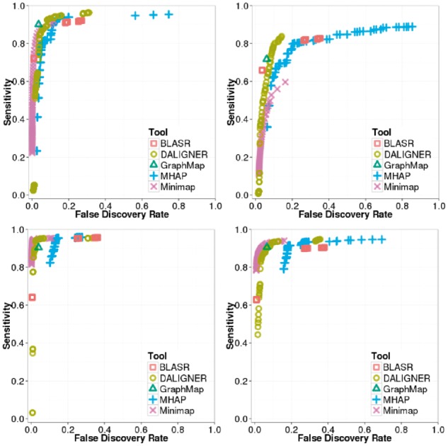
ROC-like plot using BLASR, DALIGNER, GraphMap, MHAP, GraphMap and MHAP. Top left: PB P6-C4 E.coli simulated with PBsim. Top right: PB P6-C4 E.coli dataset. Bottom left: ONT SQK-MAP-006 E.coli simulated with Nanosim. Bottom right: ONT SQK-MAP-006 E.coli dataset

We can see that although many tools have similar sensitivity and FDR depending on the parameterization, the overall trends reveal differences in sensitivity and FDR on each specific datatype. For instance, MHAP can achieve high sensitivity on all datasets, but lacks precision compared to most other methods on the ONT datasets. The only other tool that may have less precision on the ONT datasets is BLASR. DALIGNER proves to have a high sensitivity and precision, but it is not always the winner, especially on the ONT dataset. Minimap has high sensitivity and precision on the ONT datasets, but does not maintain such performance on the PB dataset. Finally, the results for GraphMap were competitive despite using a single parameterization.

These plots reveal that selection of operating parameters very much depends on the balance of project-specific importance attributed to sensitivity and precision, as expected. For instance, the importance of sensitivity is clear as it provides critical starting material for downstream processing. On the other hand, low sensitivity can be tolerated if the downstream method employs multiple iterations of error correction, because as errors are resolved within each iteration, the sensitivity is expected to increase. However, these downstream operations of course may come with a high computing cost.

The F1 score (also F-score or F-measure) represents a common way to combine the two scores we used. It is the harmonic mean between the sensitivity and precision. To better compare these methods, we computed F1 scores for each using a range of parameters, and considered the highest value for each method to be representative of its overall performance. We calculated confidence intervals for the F1 scores using three standard deviations around the observed values, which revealed that reported F1 values were statistically significantly different from each other.

For the simulated PB data, GraphMap has the highest F1 score (despite being designed for ONT data and not PB data) followed by DALIGNER, Minimap, MHAP and BLASR (Table 2). For the real PB data DALIGNER has the highest F1 score followed by GraphMap, MHAP and BLASR. For both the simulated and real ONT datasets, Minimap was the best method, yielding the highest F1 score, followed by GraphMap, MHAP and BLASR (Table 2).

Table 2.

An overview of sensitivity and precision on simulated and real error-prone long read datasets

Tool	Simulated PB E.coli			Simulated ONT E.coli			PB P6-C4 E.coli			ONT SQK-MAP-006 E.coli
	Sens. (%)	Prec. (%)	F1 (%)	Sens. (%)	Prec. (%)	F1 (%)	Sens. (%)	Prec. (%)	F1 (%)	Sens. (%)	Prec. (%)	F1 (%)
BLASR	91.0	81.9	86.2	95.2	75.1	84.0	66.0	96.5	78.3	89.9	73.0	80.6
DALIGNER	92.4	91.9	92.1	94.9	97.6	95.9	83.8	85.8	84.8	92.9	91.0	91.9
MHAP	91.5	88.0	89.8	95.1	86.5	90.6	79.8	79.8	79.8	91.2	82.0	86.3
GraphMap	90.1	96.5	93.1	90.4	96.0	93.1	71.7	94.0	81.4	90.6	93.4	92.0
Minimap	88.9	94.8	91.8	94.6	99.0	96.7	59.6	83.8	69.7	91.2	95.4	93.2

In both the PB and ONT simulated datasets, the best values, shown in bold face, are statistically significantly better than the other values. We derived these values from the best settings of each tool (according to the best F1 score) after a parameter search. We calculated confidence intervals for the sensitivity, specificity and F1 scores using three standard deviations around the observed values. In the worst case, the error never exceeded ±0.1%, ±0.1% and ±0.2% respectively.

Overall, these results suggest that some tools may perform substantially differently on data from different platforms. We hypothesize that, differences in the read length distributions and error type frequencies could be responsible for this behaviour.

5.2 Computational performance

To measure the computational performance of each method, we ran each tool with default parameters (with some exceptions see Supplementary note S2), as well as another run with optimized parameters yielding the highest F1 score (Table 2 and Supplementary note S1) obtained after a parameter sweep on the simulated datasets. We note that GraphMap’s owler mode could not be parameterized, except for choosing the number of threads, so there was no difference in the settings for default and highest F1 score parameterization runs. We ran our tests serially on the same 64-core Intel Xeon CPU E7-8867 v3 @ 2.50 GHz machine with 2.5 TB of memory. We measured the peak memory, CPU and wall clock time across read subsets to show the scalability of each method.

We investigated the scalability of the methods, testing them using 4, 8, 16 or 32 threads of execution on the E. coli datasets (Supplementary Figs S5–S12). Despite specifying the number of threads, each tool often used more or fewer threads than expected (Supplementary Figs S5, S6, S13, S14). In particular, MHAP tended to use more threads than the number we specified.

On all tested E.coli datasets in our study, we observe that Minimap is the most computationally efficient tool, robustly producing overlap regions at least 3–4 times faster than all other methods, even when parameterizing for optimal F1 score (Supplementary Figs S9, S10). Determining the next fastest method is confounded by the effect of parameterization. For instance when considering only our F1 score optimized settings, the execution time of DALIGNER was generally within an order of magnitude or less of the execution time of Minimap. On the other hand, DALIGNER can be 2–5 times slower than MHAP on some datasets under default parameters.

With default settings, DALIGNER performs up to 10 times slower than with F1 score optimized settings. This primarily occurs because the k-mer filtering threshold (-t) in the F1 optimized parameterization not only increases specificity, but also reduces runtime. In contrast, our parameterization to optimize the F1 score in MHAP decreases the speed (by a factor of 3–4). In this case, the culprit was the sketch size (–num-hashes) used; larger sketch sizes increase sensitivity at the cost of time.

Finally, GraphMap is generally the least scalable method, the slowest when considering default parameters only, and only 1–2 times faster than BLASR when considering F1 optimized settings. BLASR is also able to scale better, using more threads than GraphMap (Supplementary Figs S9, S10).

In addition to its impressive computational performance, Minimap uses less memory than almost all methods on tested E.coli datasets (Supplementary Figs S11, S12), staying within an order of magnitude of BLASR on average, despite the latter employing an FM-index. Memory usage in GraphMap seems to scale linearly with the number of reads at a rate nearly 10 times that of the BLASR or Minimap, likely owing to the hash table it uses. The memory usage characteristics of DALIGNER and MHAP are less clear, drastically changing depending on the parameters utilized. Overall MHAP has the worst memory performance even when using default parameters. The cause of the memory increase between optimized F1 and default setting in MHAP is again due to an increase in the sketch size between runs. Because of k-mer multiplicity filtering, DALIGNER’s memory usage is 2–3 times lower when parameterized for an optimized F1 score.

Many of the trends from the C.elegans datasets mirror the performance on the smaller E.coli dataset. Again, computational performance on the larger C.elegans datasets is still dominated by Minimap (Fig. 5, Supplementary Figs S13, S14), being at least 5 times faster than any other method. DALIGNER’s performance seems to generally scale well, especially when k-mer filtering is performed (within an order of magnitude of Minimap). With default settings, MHAP is 2-3 times faster than DALIGNER, but is several orders of magnitude slower, when the F1 score is optimized. The performance of GraphMap shows that it does not scale well to large number of reads (>100 000), and its calculations take an order of magnitude longer than BLASR.

Fig. 5.

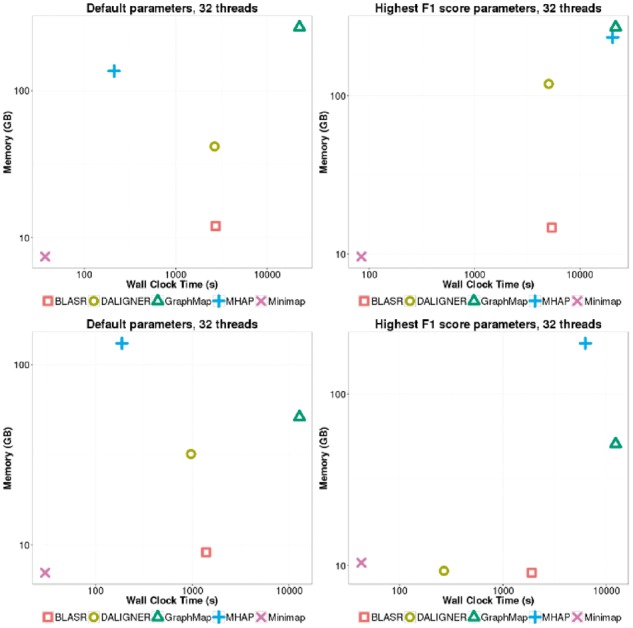
Wallclock time and memory on the PB P6-C4 (top) and simulated ONT (bottom) C.elegans dataset on 100 000 randomly sampled reads. Each tool was parameterized using default settings (left), or using settings from runs yielding the highest F1 score on the simulated E.coli datasets (right)

Of note is the performance of BLASR when run on PB and ONT datasets with default settings, which is roughly on par with that of DALIGNER (Fig. 5, Supplementary Figs S13, S14). When using optimized parameters, BLASR is also at least twice as fast as MHAP (Fig. 5, Supplementary Figs S13, S14). We had expected the computational time for DALIGNER and MHAP to scale better than BLASR on the large C.elegans datasets, as any upfront costs (e.g. MinHash sketch computation) would be amortized on larger datasets. We note that these results seemingly contradict the results found in previous studies (Berlin et al., 2015; Myers, 2014). This may be due to different datasets and technology versions used by the two studies, but to a greater extent this likely highlights the importance of careful parameterization of each tool. Specifically, for DALIGNER, it is important to filter the occurrences of k-mers (-t) in each batch to maintain not only specificity, but also computational performance. For MHAP, increasing the sketch size increases the sensitivity of the initial filter but increases computation.

The trends in memory performance on the C.elegans datasets are generally consistent with E.coli datasets (Supplementary Figs S13, S14). A notable exception however is the memory usage of DALIGNER, which begins leveling off with increased number of reads. Unlike with the E.coli dataset, this dataset is large enough that DALIGNER begins to split the data into batches, reducing its memory usage.

6 Discussion

Our study highlights that there are important considerations to factor in while developing new tools or improving existing ones.

6.1 Modularity

A tool that can report intermediate results may help reduce computation in downstream applications. For example, modularizing overlap candidate detection, overlap validation, and alignment can provide flexibility when used in different pipelines. GraphMap’s owler mode is an example of this, enabling users to generate MHAP-like output for overlap regions, rather than a more detailed alignment on detected regions. Further, compliance to standardized output is highly recommended, including for generating intermediate results. Doing so would not only allow one to perform comparative performance evaluations on a variety of equivalent metrics, but also allow for flexibility in creating new pipelines. Examples of emergent output standards include the Graphical Fragment Assembly (GFA) (https://github.com/pmelsted/GFA-spec) format, PAF (Li, 2016), and the MHAP output format.

6.2 Cache efficiency

Given the concepts presented, and along with our benchmarks performed herein indicates that theoretical performance estimations based on time complexity analysis might not be enough to conclude on what works best. Traditional algorithm complexity analysis suffers from an assumption that all memory access costs are the same. However, on modern computers intermediate levels of fast-access cache exist between the registers of the CPU and main memory. A failed attempt to read or write data in the cache is called a cache miss, causing delays by requiring the algorithm to fetch data from other cache levels or main memory.

Cache efficiency in algorithmic design has become a major consideration, and in some cases will trump many time complexity based motivations for algorithmic development. For instance, though the expected time complexity of DALIGNER has a quadratic component based on the number of occurrences of a k-mer in the dataset, its actual computational performance seems to be much better empirically. The authors claim this is due to the cache efficiency of the method (compared to using an FM-index) (Myers, 2014), and in practice this also seems to be the case, as observed in our comparisons.

The basic concept of a cache efficient algorithm relies on minimizing random access whenever possible, by serializing data accesses in blocks that are small enough to fit into various levels of cache, especially at the levels of cache with the lowest latency. Algorithms that exploit a specific cache configuration utilize an I/O-model (also called the external-memory model) (Aggarwal et al., 1988; Demaine, 2002). Conceptually, these algorithms must have explicit knowledge of the size of each component of the memory hierarchy, and will adjust the size of contiguous blocks of data to minimize data transfers from memory to cache.

In contrast to the I/O model, algorithms that are designed with cache in mind, but do not explicitly rely on known cache size blocks are called cache oblivious (Frigo et al., 1999). Cache oblivious algorithms are beneficial, as they do not rely on the knowledge of the processor architecture; instead they utilize classes of algorithms that are inherently cache efficient such as scanning algorithms (e.g. DALIGNER’s merging step of a sorted list).

6.3 Batching and batch/block sizes

For many of the methods surveyed in this paper, memory usage scales linearly to the number of reads in the set, sometimes exceeding 100 GB on only 100 000 long reads (Fig. 5, Supplementary Fig. S12, S13). Thus, to perform all necessary comparisons on large datasets (i.e. to compute an upper triangular matrix of candidate comparisons) the data must be processed in batches. Generally, it is better to use as few blocks as possible, since the time required to perform all overlaps is quadratic relative to the number of batches. Methods that have a very low memory usage overall will be able to have the computational benefit of splitting the data into fewer batches. Batching is handled in different ways depending on the tool. Some tools have built-in splitting (DALIGNER/DAZZLER database with DBsplit and -I with Minimap), and others have this process built into their associated pipelines (e.g. MHAP and PBcR). Though BLASR may have more scalable memory usage, it will eventually require splitting as the index it uses is limited to 4 GB in size. To encourage the adoption of a tool in different pipeline contexts, built-in batching is a desirable attribute to ensure that memory usage scales with the dataset size.

6.4 Repetitive elements and sequence filtering

Any common regions due to homology or other repetitive elements may confound read-to-read overlaps, and may be difficult to disambiguate from true overlaps. Such repetitive elements may lead to many false positives in overlap detection, and may increase the computational burden, leading to lower quality in downstream assembly. Thus, it is common for overlap methods to employ sequence filtering, by removal or masking of repetitive elements to improve algorithmic performance both in run time and specificity. Many of the methods compared utilize k-mer frequencies to filter highly repetitive k-mers using an absolute or percent k-mer multiplicity (e.g. MHAP). These filtering approaches can be affected by the batch size when filters are seeded based on their multiplicity in each batch, rather than in the entire dataset (e.g. DALIGNER, Minimap). Another common filtering strategy is to prevent the use of low complexity sequences (e.g. DALIGNER, Minimap).

Some overlaps caused by repetitive elements can be useful for some assembly pipelines, such as in the identification of repeat boundaries. Thus, provided that it is computationally tractable, it may be beneficial for future overlap algorithms to assess the likelihood that an overlap is repeat-induced; this metric would ideally be standardized to facilitate modularity between pipelines.

6.5 Tuning for sensitivity and specificity

As we have presented in our review, methods to compute read-to-read overlap vary in their designs and implementations, although they share similar concepts and parameters. For example, many of the methods are k-mer based and, as expected, behave similarly when that parameter is tuned; for instance, increasing k increases specificity but decreases sensitivity especially on sequencing data with high base error. At the current error rates for both PB and ONT technologies, a k of 16 is optimal, but it can be expected to increase as error rates decrease.

Another common theme amongst read overlap tools is that, many methods employ an initial candidate discovery stage, followed with a more specific candidate validation stage. Increasing sensitivity at the cost of specificity at the initial stage is typically tolerated by the second stage. However, because the second stage is often computationally expensive, one must accordingly tune parameters such as –nCandidates in BLASR, which control the number candidates considered for the validation stage.

Growing in popularity is the use of another prominent method, minimizers (e.g. MinHash sketches), to generate a reduced representation of each sequence to help reduce memory usage and speed-up comparisons. In this approach, tuning the corresponding parameters (e.g. –w in Minimap and –num-hashes in MHAP) in a way that more closely traces the original data representation will result in higher sensitivity and sensitivity, but at a greater computational cost.

7 Conclusions

There are many challenges in evaluating algorithms that function on error-prone long reads, such as those from PB and ONT instruments. Although both sequencing technologies have comparable error rates, characteristics of their errors as well as their read length distributions are substantially different. Also, within each technology there are rapid improvements in quality (Jain et al., 2015; Laver et al., 2015), causing disagreement between datasets derived from the same technology.

Despite these issues, we show that Minimap is the most computationally efficient method (in both time and memory) and is the most specific and sensitive method on the ONT datasets tested. We note that Minimap is not as sensitive or as specific as Graphmap, DALIGNER or MHAP on the PB datasets tested. Our results shown that GraphMap and DALIGNER are most specific and sensitive method on PB datasets tested, though DALIGNER scales better computationally. PB being a more mature technology compared to ONT, it is not surprising to see several tools performing well on the platform.

Here, we have provided an overview of leading read-to-read overlap detection methods, comparing their concepts and performances. We think our results will guide researchers to make informed decisions when choosing between these methods. As well, our elucidation to open problems may help developers improve on existing overlap detection tools, or build new ones.

References

- Aggarwal A. et al. (1988) The input/output complexity of sorting and related problems. Commun. ACM, 31, 1116–1127. [Google Scholar]
- Alkan C. et al. (2010) Limitations of next-generation genome sequence assembly. Nat. Methods, 8, 61–65. [DOI] [PMC free article] [PubMed] [Google Scholar]
- Benson G. et al. (2013) Longest common subsequence in k Length Substrings. In: International Conference on Similarity Search and Applications. Springer Berlin Heidelberg, pp. 257–265.
- Berlin K. et al. (2015) Assembling large genomes with single-molecule sequencing and locality-sensitive hashing. Nat. Biotechnol., 33, 623–630. [DOI] [PubMed] [Google Scholar]
- Boža V. et al. (2016) DeepNano: Deep Recurrent Neural Networks for Base Calling in MinION Nanopore Reads. arXiv preprint arXiv:1603.09195. [DOI] [PMC free article] [PubMed]
- Broder A.Z. (1997) On the resemblance and containment of documents. In: Proceedings Compression and Complexity of SEQUENCES 1997 (Cat. No.97TB100171) IEEE, pp. 21–29.
- Burkhardt S. et al. (2002) One-Gapped q-Gram Filters for Levenshtein Distance. In: Annual Symposium on Combinatorial Pattern Matching. Springer Berlin Heidelberg. pp. 225–234
- Carneiro M.O. et al. (2012) Pacific biosciences sequencing technology for genotyping and variation discovery in human data. BMC Genomics, 13, 375.. [DOI] [PMC free article] [PubMed] [Google Scholar]
- Chaisson M.J., Tesler G. (2012) Mapping single molecule sequencing reads using basic local alignment with successive refinement (BLASR): application and theory. BMC Bioinformatics, 13, 238.. [DOI] [PMC free article] [PubMed] [Google Scholar]
- Chin C.S. et al. (2013) Nonhybrid, finished microbial genome assemblies from long-read SMRT sequencing data. Nat. Methods, 10, 563–569. [DOI] [PubMed] [Google Scholar]
- David M. et al. (2016) Nanocall: An Open Source Basecaller for Oxford Nanopore Sequencing Data. bioRxiv, 046086. [DOI] [PMC free article] [PubMed]
- Demaine E.D. (2002) Cache-oblivious algorithms and data structures. Lect. Notes EEF Summer School Massive Data Sets, 8, 1–249. [Google Scholar]
- Eid J. et al. (2009) Real-time DNA sequencing from single polymerase molecules. Science, 323, 133–138. [DOI] [PubMed] [Google Scholar]
- Eisenstein M. (2015) Startups use short-read data to expand long-read sequencing market. Nat. Biotechnol., 33, 433–435. [DOI] [PubMed] [Google Scholar]
- Ewing B. et al. (1998) Base-calling of automated sequencer traces usingPhred. I. Accuracy assessment. Genome Res., 8, 175–185. [DOI] [PubMed] [Google Scholar]
- Ferragina P. et al. (2005) Indexing compressed text. J. ACM, 52, 552–581. [Google Scholar]
- Frigo M. et al. (1999) Cache-oblivious algorithms. In: 40th Annual Symposium on Foundations of Computer Science, 1999. IEEE, pp. 285–297.
- Goodwin S. et al. (2015) Oxford nanopore sequencing, hybrid error correction, and de novo assembly of a eukaryotic genome. Genome Res., 25, 1750–1756. [DOI] [PMC free article] [PubMed] [Google Scholar]
- Jain M. et al. (2015) Improved data analysis for the MinION nanopore sequencer. Nat. Methods, 12, 351–356. [DOI] [PMC free article] [PubMed] [Google Scholar]
- Jiao X. et al. (2013) A benchmark study on error assessment and quality control of CCS reads derived from the PacBio RS. J. Data Min. Genomics Proteomics, 4, 1–5. [DOI] [PMC free article] [PubMed] [Google Scholar]
- Keich U. et al. (2004) On spaced seeds for similarity search. Discrete Appl. Math., 138, 253–263. [Google Scholar]
- Laehnemann D. et al. (2016) Denoising DNA deep sequencing data-high-throughput sequencing errors and their correction. Brief. Bioinform., 17, 154–179. [DOI] [PMC free article] [PubMed] [Google Scholar]
- Laver T. et al. (2015) Assessing the performance of the Oxford Nanopore Technologies MinION. Biomol. Detect. Quantif., 3, 1–8. [DOI] [PMC free article] [PubMed] [Google Scholar]
- Levene M.J. et al. (2003) Zero-mode waveguides for single-molecule analysis at high concentrations. Science, 299, 682–686. [DOI] [PubMed] [Google Scholar]
- Li H. (2016) Minimap and miniasm: fast mapping and de novo assembly for noisy long sequences, Bioinformatics, 25, 1754–1760. [DOI] [PMC free article] [PubMed]
- Li H., Durbin R. (2009) Fast and accurate short read alignment with Burrows-Wheeler transform. Bioinformatics, 25, 1754–1760. [DOI] [PMC free article] [PubMed] [Google Scholar]
- Loman N.J. et al. (2015) A complete bacterial genome assembled de novo using only nanopore sequencing data. Nat. Methods, 12, 733–735. [DOI] [PubMed] [Google Scholar]
- Marçais G., Kingsford C. (2011) A fast, lock-free approach for efficient parallel counting of occurrences of k-mers. Bioinformatics, 27, 764–770. [DOI] [PMC free article] [PubMed] [Google Scholar]
- McCoy R.C. et al. (2014) Illumina TruSeq synthetic long-reads empower de novo assembly and resolve complex, highly-repetitive transposable elements. PLoS One, 9, e106689.. [DOI] [PMC free article] [PubMed] [Google Scholar]
- Morgulis A. et al. (2006) A Fast and Symmetric DUST Implementation to Mask Low-Complexity DNA Sequences. J. Comp. Biol., 13, 1028–1040. [DOI] [PubMed]
- Myers E.W. (2000) A whole-genome assembly of Drosophila. Science, 287, 2196–2204. [DOI] [PubMed] [Google Scholar]
- Myers G. (2014) Efficient local alignment discovery amongst noisy long reads In: International Workshop on Algorithms in Bioinformatics. Springer Berlin Heidelberg, pp. 52–67. [Google Scholar]
- O'Donnell C.R. et al. (2013) Error analysis of idealized nanopore sequencing. Electrophoresis, 34, 2137–2144. [DOI] [PMC free article] [PubMed] [Google Scholar]
- Ono Y. et al. (2013) PBSIM: PacBio reads simulator–toward accurate genome assembly. Bioinformatics, 29, 119–121. [DOI] [PubMed] [Google Scholar]
- Quick J. et al. (2014) A reference bacterial genome dataset generated on the MinION™ portable single-molecule nanopore sequencer. Gigascience, 3, 22.. [DOI] [PMC free article] [PubMed] [Google Scholar]
- Richards S., Murali S.C. (2015) Best practices in insect genome sequencing: what works and what doesn’t. Curr. Opin. Insect Sci., 7, 1–7. [DOI] [PMC free article] [PubMed] [Google Scholar]
- Ross M.G. et al. (2013) Characterizing and measuring bias in sequence data. Genome Biol., 14, R51.. [DOI] [PMC free article] [PubMed] [Google Scholar]
- Simpson J.T., Mihai P. (2015) The theory and practice of genome sequence assembly. Annu. Rev. Genomics Hum. Genet., 16, 153–172. [DOI] [PubMed] [Google Scholar]
- Smith D.R. et al. (2008) Rapid whole-genome mutational profiling using next-generation sequencing technologies. Genome Res., 18, 1638–1642. [DOI] [PMC free article] [PubMed] [Google Scholar]
- Smith T.F., Waterman M.S. (1981) Identification of common molecular subsequences. J. Mol. Biol., 147, 195–197. [DOI] [PubMed] [Google Scholar]
- Sović I. et al. (2016) Fast and sensitive mapping of nanopore sequencing reads with GraphMap. Nat. Commun., 7, 11307.. [DOI] [PMC free article] [PubMed] [Google Scholar]
- Sović I. et al. (2016) Evaluation of hybrid and non-hybrid methods for de novo assembly of nanopore reads, Bioinformatics, 32, 2582–2589. [DOI] [PubMed] [Google Scholar]
- Stoddart D. et al. (2009) Single-nucleotide discrimination in immobilized DNA oligonucleotides with a biological nanopore. Proc. Natl. Acad. Sci. U. S. A., 106, 7702–7707. [DOI] [PMC free article] [PubMed] [Google Scholar]
- Travers K.J. et al. (2010) A flexible and efficient template format for circular consensus sequencing and SNP detection. Nucleic Acids Res., 38, e159.. [DOI] [PMC free article] [PubMed] [Google Scholar]
- Treangen T.J., Salzberg S.L. (2012) Repetitive DNA and next-generation sequencing: computational challenges and solutions. Nat. Rev. Genet., 13, 36–46. [DOI] [PMC free article] [PubMed] [Google Scholar]
- Ummat A., Bashir A. (2014) Resolving complex tandem repeats with long reads. Bioinformatics, 30, 3491–3498. [DOI] [PubMed] [Google Scholar]
- Wang J.R., Jones C.D. (2015) Fast alignment filtering of nanopore sequencing reads using locality-sensitive hashing. In: 2015 IEEE International Conference on Bioinformatics and Biomedicine (BIBM).
- Yang C. et al. (2016) NanoSim: nanopore sequence read simulator based on statistical characterization. bioRxiv, 044545. [DOI] [PMC free article] [PubMed]
Associated Data
This section collects any data citations, data availability statements, or supplementary materials included in this article.