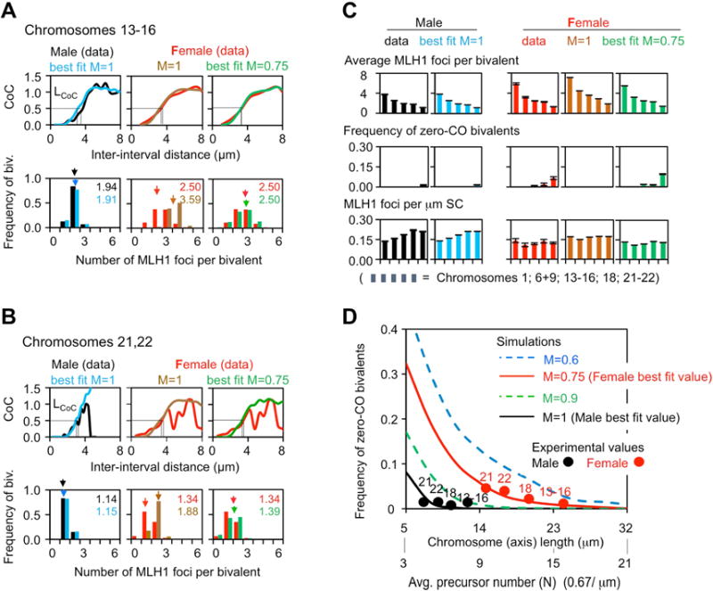
Figure 3. Simulation analysis of male and female CO patterns.

CO patterns from MLH1 focus analysis (male black and female red) were compared with patterns predicted from fill-in-the-holes simulation analyses performed under conditions of interest (text; STAR Methods). (A,B) Descriptions for two groups of similar chromosomes: 13–16 (A) and 21–22 (B). Top: Coefficient of Coincidence (CoC) curves; bottom: frequencies of bivalents with different numbers of COs (and the average). For CoC analysis, each chromosome is divided into a series of intervals. CoC is the ratio of the frequency of “observed” double COs to the frequency of “expected ”double COs, which is defined by the product of the CO frequencies in each of the two component intervals considered individually. A CoC curve plots this ratio, for every pair of intervals, as a function of inter-interval distance. In the presence of CO interference, the frequency of double COs is much lower than expected for closely-spaced intervals, increases to the level expected for independent occurrence (CoC = 1), and then fluctuates around that value due to the tendency for even spacing (STAR Methods and Figure S1). No rigorous statistical test exists to evaluate the difference between two CoC curves. However, a sensitive and reliable quantitative indicator is the inter-interval distance at which CoC = 0.5, “LCoC” (STAR Methods). Examples of non-matching CoC curves are in Figure S3. (C) The goodness-of-fit of each simulated CO number distribution per bivalent as compared to the experimental data was evaluated by the sum of the squares of the differences (SSD): Chromosome 13–16: female M=1, SSD=0.353; M=0.75, SSD=0.004. Chromosomes 21, 22: female M=1, SSD=0.349; M=0.75, SSD=0.025. (D) Simulation-predicted frequencies of zero-CO bivalents as a function of chromosome length (or, equivalently, number of “precursors”, i.e. DSBs) at different levels of maturation efficiency (“M”) (STAR Methods). Note close matches of experimental (filled circles) and predicted (curves) values. See also Figures 4B, S2–S4. MLH1 data in Table S1.
