Abstract
Microarray measurements of gene expression constitute a large fraction of publicly shared biological data, and are available in the Gene Expression Omnibus (GEO). Many studies use GEO data to shape hypotheses and improve statistical power. Within GEO, the Affymetrix HG-U133A and HG-U133 Plus 2.0 are the two most commonly used microarray platforms for human samples; the HG-U133 Plus 2.0 platform contains 54 220 probes and the HG-U133A array contains a proper subset (21 722 probes). When different platforms are involved, the subset of common genes is most easily compared. This approach results in the exclusion of substantial measured data and can limit downstream analysis. To predict the expression values for the genes unique to the HG-U133 Plus 2.0 platform, we constructed a series of gene expression inference models based on genes common to both platforms. Our model predicts gene expression values that are within the variability observed in controlled replicate studies and are highly correlated with measured data. Using six previously published studies, we also demonstrate the improved performance of the enlarged feature space generated by our model in downstream analysis.
Availability and Implementation
The gene inference model described in this paper is available as a R package (affyImpute), which can be downloaded at http://simtk.org/home/affyimpute.
Supplementary information
Supplementary data are available at Bioinformatics online.
1 Introduction
The Gene Expression Omnibus (GEO) is a public repository for genomic data supported by the National Center for Biotechnology Information (NCBI), containing nearly two million samples and growing. GEO enables multiple uses of expression datasets individually and in combination, and is a rich resource for bench researchers and bioinformaticians. Although we recognize that RNA-sequencing is becoming the dominant mode for conducting gene expression analysis, microarray-based studies continue to be important, with over 4000 microarray studies added to GEO within the past year. As of 1st Jan 2016, there are approximately one million human samples (987 744) in GEO, half of which are based on in situ oligonucleotide technology. The Affymetrix HG-U133 Plus 2.0 and HG-U133A are the two most prevalent microarray platforms, collectively comprising one third of all such samples. Data from many widely used landmark projects are based on these two platforms. For instance, the Connectivity Map (Lamb, 2007; Lamb et al., 2006), Genomics of Drug Sensitivity in Cancer (Yang et al., 2013) and the Cancer Cell Line Encyclopedia (CCLE) (Barretina et al., 2012) use the high-throughput version of the HG-U133A array for gene expression analysis, whereas The Cancer Genome Atlas (TCGA) uses the HG-U133 Plus 2.0 platform. Some of these resources are not deposited in GEO, so the number of samples in GEO is in fact an underestimate of the amount of available genomic data from the two platforms. Facilitating the analysis of data between the two platforms will extend the usefulness of these valuable public resources.
The HG-U133A and Plus 2.0 platforms are based on the UniGene Human Database release 133 (media.affymetrix.com/support/tech notes/hgu133_design_technote.pdf), but differ in the number of probe sets and represented genes. The HG-U133A array is actually one half of the Affymetrix HG-U133 set, HG-U133B being the other array which focuses mostly on expressed sequence tags. The newer HG-U133 Plus 2.0 platform adds approximately 10 000 probe sets to the combined HG-U133 set, representing an increase of 6500 genes analyzed (Supplementary Fig. S1). When studies involve the use of data arising from both platforms, typically only probes that are common to both platforms are retained for downstream analysis; since the HG-U133A probe sets are fully contained in HG-U133 Plus 2.0, this means restricting the data to the size of the HG-U133A array.
Although rarely acknowledged, the truncation of data can affect any downstream analysis and is ultimately wasteful. For instance, correlation-based methods used in clustering samples can produce significantly different results when the feature size is reduced. Computational methods such as the Gene Set Enrichment Analysis (GSEA) assigns NA values to genes that were truncated from the HG-U133 Plus 2.0 array, excluding them from all further analysis. Although the truncation of data may have been justifiable back when HG-U133A platform was the most common platform, the increasing proportion of HG-U133 Plus 2.0 samples (Fig. 1) in public repositories suggests that the amount of discard ed data is no longer negligible. In fact, the growth in the number of HG-U133A samples is likely to eventually stagnate: the HG-U133A and B platforms have been discontinued at present, and can only be custom ordered in whole lots from Affymetrix. Nonetheless, the substantial previous investment should be maintained as a usable resource as long as possible.
Fig. 1.
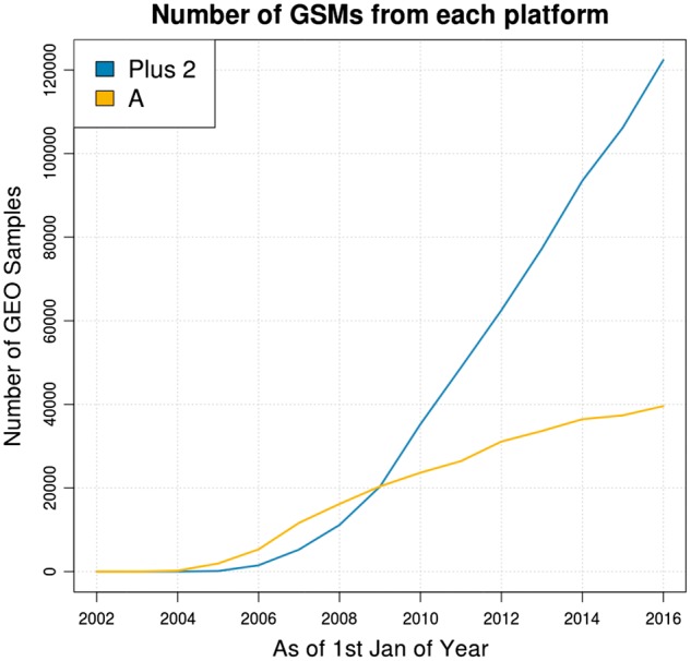
Number of GEO samples from each platform over time. The sample counts were limited to only human samples
There is evidence that measurements from the same probes on the two platforms are directly comparable (media.affymetrix.com/support/technotes/hgu133_p2_technote.pdf), and the vast majority of papers published in the last decade using these two platforms have relied on this. We hypothesize that the high correlation between gene expression values allows us to predict the gene expression values for the genes measured only in the HG-U133 Plus 2.0 platform with high accuracy. In this work, we use the large amount of data in GEO to build prediction models that can bring data measured on the HG-U133A space to the larger feature space in HG-U133 Plus 2.0. We show that we can achieve high accuracy with our predicted gene expression values, and that the increased data dimension improves downstream biological analysis.
2 Methods
All analysis and model building were done using R 3.2.0 (R Core Team, Vienna, Austria).
2.1 Data for model
We restricted our GEO query to human samples and selected all series records (GSEs) as of March 2015 that were based on the Affymetrix HG-U133 Plus 2.0 platform. Each GSE was then mapped to its corresponding samples (GSMs). If a GSM appeared in more than one GSE, we assigned it to the oldest GSE. GSMs without associated microarray CEL files were treated as invalid for our purposes, and only GSEs containing at least three valid samples were retained. In total, 97 049 microarray CEL files, coming from 2753 accepted GSEs, were downloaded. The R packages GEOquery (Davis and Meltzer, 2007) and GEOmetadb (Zhu et al., 2008) were used to perform the above tasks.
The CEL files within each GSE were processed using robust multi-array average (RMA) (Bolstad et al., 2003; Gautier et al., 2004). Technical bias correction was done using the R package bias v0.0.5 (Eklund and Szallasi, 2008). The probe sets were then mapped to Entrez gene identifiers using the R package Jetset v3.1.2 (Li et al., 2011). The mapping from Jetset yielded 20 089 and 12 210 unique Entrez gene identifiers for the HG-U133 Plus 2.0 and HG-U133A platforms respectively, with the latter being a proper subset of the former. Of these, only 10 103 Entrez gene identifiers were obtained from the same probes on both platforms. We refer to these 10 103 genes as the ‘common gene set’ (Fig. 2).
Fig. 2.
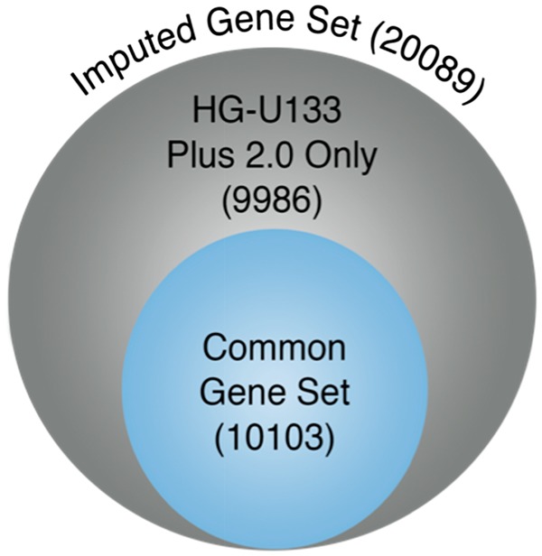
Venn diagram depicting the common and imputed gene sets
2.2 Gene models
We built LASSO models (R package glmnet (Friedman et al., 2010)) independently for each of the 9986 genes found only on the HG-U133 Plus 2.0 platform, using the common gene set as predictors. A set of 20 049 arrays were randomly chosen and held-out as a test set, while the remaining 77 000 arrays were used to train the gene models. Ten-fold cross-validation was performed on the training set to determine the regularization parameter λ. We retained the coefficients corresponding to λmin, the value of λ that gave the minimum mean cross-validated error, and also λ1se, the largest λ for which the error is within one standard error of the minimum error. We refer to the collective set of coefficients as our model, with two possible choices of coefficient matrices based on λmin and λ1se. The analyses presented in this paper were performed using the λ1se coefficient matrix. Both coefficient matrices can be obtained at http://simtk.org/home/affyimpute.
2.3 Analysis of model performance
Predictions of gene expression were done on the held-out test set comprising 20 049 arrays. The predicted gene levels were compared with the measured levels to get the root-mean-squared error (RMSE) for each gene model. To account for the differences in magnitude across the 9986 genes, we used the coefficient of variance of RMSE, CV(RMSE), which is defined as:
where and are the RMSE and mean value of gene respectively.
Separately, we downloaded the Affymetrix HGU-133 Plus 2.0 data from the MicroArray Quality Control (MAQC) Project (GSE5350) (MAQC et al., 2006), which contains four sample types based on the Universal Human Reference RNA (UHRR) from Stratagene and the Human Brain Reference RNA (HBRR) from Ambion: Sample A, 100% UHRR; Sample B, 100% HBRR; Sample C, 75% UHRR:25% HBRR; Sample D, 25% UHRR:75% HBRR. Each sample was tested in six different institutes, with five replicates done in each of the institutes, yielding a total of 30 samples per sample type. Greater detail on the protocol is provided in the original paper from MAQC. We processed the data for each sample type independently as per the methods described in the earlier section (‘Data for Model’). For each sample type, we obtained the unbiased estimate of the coefficient of variation (Haldane, 1955; Sokal and Braumann, 1980) for each of the 9986 genes using the formula:
where is the number of samples of a particular type, and are the standard deviation and mean value of gene i respectively.
2.4 Human disease network genes and MSigDB signatures
We obtained the curated table of diseases and OMIM IDs from Supplementary Table S1 of Goh et al. (2007), and mapped the 1752 unique OMIM IDs to their corresponding Entrez IDs using the mim2gene file from OMIM (www.omim.org).
We downloaded the eight gene set collections from MSigDB v5.1 (Subramanian et al., 2005) based on the Entrez IDs. For each gene signature in a collection (C1: positional, C2: curated, C3: motif, C4: computational, C5: Gene Ontology, G6: oncogenic signatures, C7: immunologic signatures, H: hallmark), the percentage overlap with the genes from each array was computed.
2.5 Evaluation sets
All external evaluation datasets were downloaded separately from GEO and processed using RMA (Bolstad et al., 2003; Gautier et al., 2004). We then mapped the probe sets to Entrez gene identifiers using Jetset and predicted the expression level of genes not measured in the HG-U133A platform using our model. We define the gene set, comprising of the measured genes on the HG-U133A platform and the predicted genes, as the ‘imputed gene set’ (Fig. 2), and the corresponding transformed HG-U133A sample as the ‘imputed sample’.
To evaluate the accuracy of our model, we used three previously published works (GSE17700 (Symmans et al., 2010), GSE23906 (Wen et al., 2010) and GSE3061 (Zhang et al., 2006)) that assessed the concordance of data from both platforms. These three studies consist of samples that were measured using both the HG-U133A and the HG-U133 Plus 2.0 platforms. We compared the 9986 imputed HG-U133 Plus 2.0 genes to those measured on the HG-U133 Plus 2.0 array using Spearman’s correlation. We additionally correlated the imputed sample of 20 089 genes to the measured sample to assess the similarity of using the imputed versus measured values of the imputed gene set in downstream analysis.
We also applied our model to another three studies (GSE11482 (Gadd et al., 2010), GSE3893 (Schuetz et al., 2006) and GSE26712 (Bonome et al., 2008)) to demonstrate the effect of the increased number of features on downstream data analysis. GSE11482 consists of 53 samples representing four different types of pediatric kidney tumors measured on the HG-U133A platform. We performed hierarchical clustering (using 1-Spearman’s correlation as the metric) on the samples restricted to the common gene set as defined previously and also on the imputed samples.
In analyzing GSE3893 and GSE26712, we applied the methods described in the original papers to the samples, filtered by (i) the full probe set used in the original work, (ii) the common gene set and (iii) the imputed gene set. GSE3893 consists of 24 breast cancer samples from 20 tumors with ductal carcinoma in situ (DCIS) and invasive ductal carcinoma (IDC). Ten samples were profiled using the HG-U133A array, and the remaining 14 samples used the HG-U133 Plus 2.0 array. We constructed imputed samples from the HG-U133A samples, and used these alongside the original HG-U133 Plus 2.0 samples in our analysis. For their analysis, Schuetz et al. performed hierarchical clustering using the neighbor-joining method with 1-Pearson’s correlation as the distance metric. We applied the same method using the ape v.3.4 package (Paradis et al., 2004) to the original data and the imputed arrays.
For GSE26712, Bonome et al. derived a gene signature to predict survival in suboptimally debulked ovarian carcinoma patients and validated their signature in an independent dataset from Berchuck et al. (2005). In concordance with their methods, we constructed univariate Cox proportional hazards models for each gene. Genes with p-value less than 0.01 were used to form a gene signature to differentiate long and short survival time in suboptimally debulked ovarian cancer patients. A compound covariate regression model was constructed using the significant genes from GSE26712 and tested on the data from Berchuck et al. Data from both studies were median-adjusted as done in Bonome et al. Validation data was obtained via the R package FULLVcuratedOvarianData (Ganzfried et al., 2013), which contained 28 of the original 29 suboptimally debulked ovarian cancer samples (Berchuck et al., 2005). We evaluated performance on the validation data using the chi-squared test as done in Bonome et al. We assigned short survival, or poor prognosis, patients as the positive case, and we further measured performance using accuracy, precision, recall and the F1 measure.
3 Results
3.1 Analysis of model performance
The distribution of test set CV(RMSE) across the gene models indicates that the vast majority of the gene models had a low CV(RMSE) around 0.05 (Fig. 3). Analysis of the ten genes with the highest test CV(RMSE) showed that the error distributions are heavy tailed, with the median absolute error for each gene being less than 0.5 (Supplementary Fig. S2A). These errors are typically less than 10% of the mean gene expression value (Supplementary Fig. S2B). Although the coefficient of variation for each of the four sample types from the MAQC project were generally slightly lower, the ranges are comparable (Fig. 4). The test set CV(RMSE) had a maximum value of 0.206 whereas the maximum CVs for the MAQC sample types were between 0.181 and 0.226.
Fig. 3.
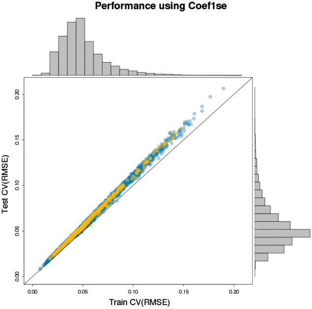
Test and training CV(RMSE). Each colored circle represents a gene model. The marginal histograms show the distribution of errors across the 9986 gene models. The 365 gene models from the Human Disease Network are depicted in orange
Fig. 4.
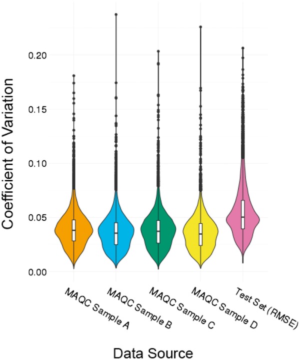
Coefficient of variation of MAQC data (in comparison with test CV(RMSE))
The analysis of genes from the Human Disease Network yielded 1643 unique Entrez IDs, of which 365 were in our set of 9986 predicted genes. The mean and median test CV(RMSE) of the corresponding 365 gene models were 0.0625 and 0.0537, respectively, and the standard deviation was 0.0294.
3.2 Signatures from MSigDB
The default settings of gene set enrichment analysis (GSEA) (Subramanian et al., 2005) are to ignore any signature that has fewer than 25 genes, or more than 500 genes. Table 1 shows the number of gene signatures in each MSigDB collection that are retained when the two platforms are used. There were cases where a gene signature was not retained for testing when the smaller HG-U133A platform was used, but would have been retained if HG-U133 Plus 2.0 were used. For the C2 collection, there were 128 of these cases, accounting for nearly 3% of signatures in the collection. For the other collections, such cases accounted for 0.5–1%, with the notable exceptions of the C7 and H collections which each had zero, and the C1 collection which had 18%.
Table 1.
Gene overlap between MSigDB collections and platforms
| Collection |
||||||||
|---|---|---|---|---|---|---|---|---|
| H | C1 | C2 | C3 | C4 | C5 | C6 | C7 | |
| Total number of valid signatures | 50 | 271 | 2949 | 752 | 702 | 737 | 186 | 1910 |
| Overlap with HG-U133A | 50 | 156 | 2752 | 747 | 680 | 664 | 184 | 1910 |
| Overlap with HG-U133 Plus 2.0 | 50 | 215 | 2880 | 752 | 689 | 715 | 186 | 1910 |
A valid signature contains between 25 and 500 genes.
3.3 Evaluation sets
3.3.1 GSE3061, GSE17700, GSE23906
Our imputed gene samples showed high correlation with the original measured HG-U133 Plus 2.0 gene samples, with mean Spearman correlation coefficients of 0.90 ± 0.012, 0.96 ± 0.005 and 0.94 ± 0.004 for GSE3061, GSE17700 and GSE23906, respectively. The corresponding heatmaps for the sample-wise comparison for these three studies are shown in Supplementary Figures S3–S5. Comparing only the 9986 predicted genes showed similar performance with correlation coefficients of 0.89 ± 0.012, 0.95 ± 0.006 and 0.92 ± 0.009 for the three respective studies. Overall, sample correlation coefficients ranged from 0.87 to 0.97, and correlation coefficients for the subset of predicted genes ranged from 0.87 to 0.95. Supplementary Figure S3B shows that predicted genes lie close to the identity line, indicating that the imputed sample closely mimics the measured sample at the individual gene level.
3.3.2 GSE3893
In replicating the hierarchical clustering on the nine sets of patient tumors in GSE3893 (Fig. 5A), we recreated the original dendrogram in Figure 2 of Schuetz et al. (Fig. 5B). Figure 5C shows the hierarchical clustering when we use the imputed samples. Notably, the estrogen receptor (ER) positive and ER negative subclusters are preserved, and IDC and DCIS samples from the same tumor remain linked. Though the dendrogram structures closely resemble each other, the use of the imputed sample s resulted in tumor 2 clustering with tumors 8 and 3 in the ER positive subgroup instead of with tumors 4, 6 and 7.
Fig. 5.
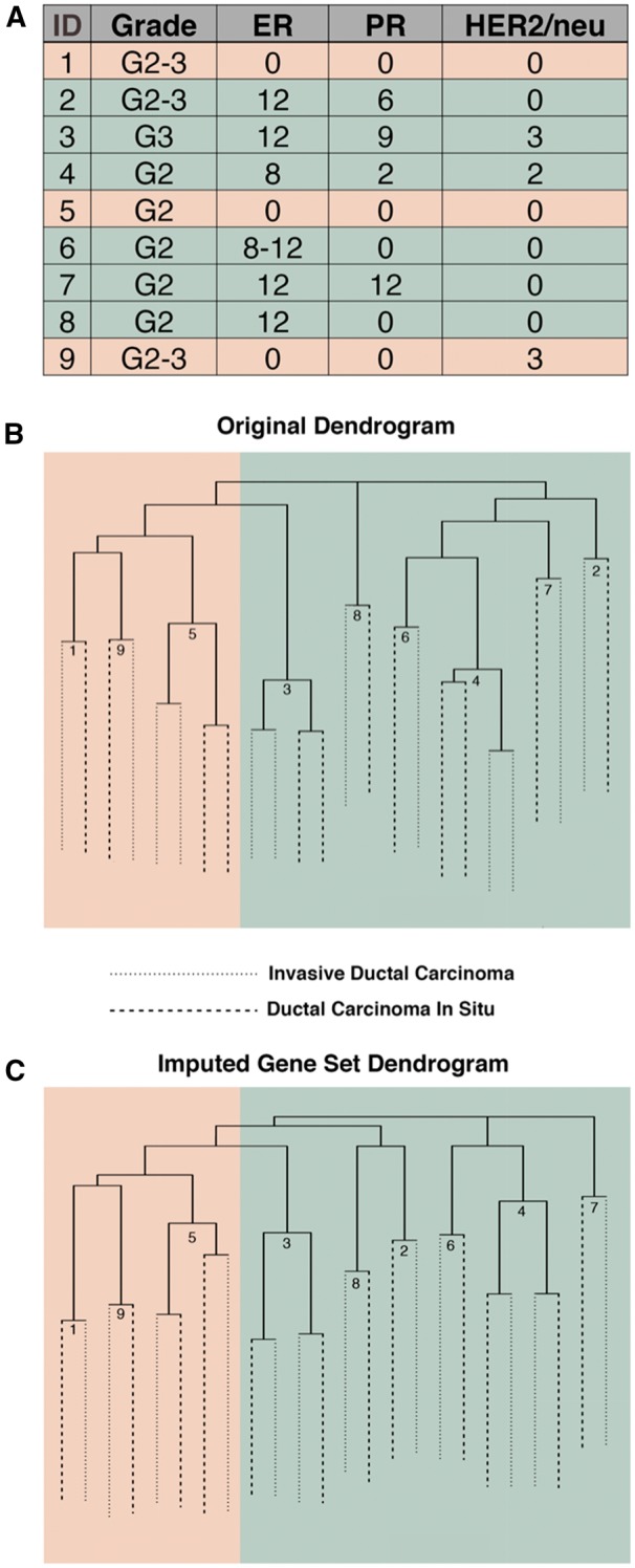
Tumor grade and estrogen receptor (ER), progesterone receptor (PR) and HER2/neu immunoreactive scores for patients in GSE3893 (A). Hierarchical clustering of breast cancer tumors from GSE3893 using the original HG-U133A probes (B) and the imputed HG-U133 Plus 2.0 array (C)
3.3.3 GSE11482
When hierarchical clustering was done using only the common gene set, we observed four distinct clusters of kidney tumors, one corresponding to each tumor type (Fig. 6). However, one of the cellular mesoblastic nephroma (CMN) samples erroneously associated with the Wilms tumors (WT). Using the imputed genes produced four homogeneous clusters while maintaining the general substructure within clusters observed originally. There is a slight restructuring in the upper branches of the tree, where CMN is now more closely associated with clear cell sarcoma of the kidney (CCSK) than the other two tumor types.
Fig. 6.
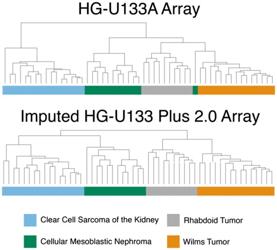
Hierarchical clustering of kidney tumors using the HG-U133A array and the imputed HG-U133 Plus 2.0 array
3.3.4 GSE26712
Bonome et al. reported 572 HG-U133A probes to be significantly associated with survival time in the suboptimally debulked ovarian cancer patients. Our univariate Cox models yielded 323 and 588 significant genes in the common and imputed gene sets, respectively. We found that a cutoff score of 0 using the original 572 probes divided the training data into 50 patients with good prognosis and 45 patients with poor prognosis, matching the data presented in Figure 2 of Bonome et al.Table 2 shows the classification results from applying our regression models to the validation data for each gene set, together with the original results as described in Bonome et al. Limiting the analysis of the imputed genes to the most significant 572 yielded the same classification results as using the entire set of 588 genes.
Table 2.
Performance results of gene signature models in distinguishing long from short survival on external validation data
| Gene set | Accuracy | Precision | Recall | F1 Measure | Chi-squared P-value |
|---|---|---|---|---|---|
| Original Probes (N = 572) | 0.759 | 0.789 | 0.833 | 0.811 | 0.029 |
| Common Genes (N = 323) | 0.643 | 0.786 | 0.611 | 0.689 | 0.236 |
| Imputed Genes (N = 588) | 0.786 | 0.800 | 0.889 | 0.842 | 0.021 |
4 Discussion
GEO represents a large trove of data for mining and inference and has enabled many valuable secondary analyses (termed by some as ‘research parasitism’ (Longo and Drazen, 2016)). In this work, we take advantage of a large collection of publicly available arrays to develop a statistical model that combines two of the most popular microarray platforms for downstream analysis. The expression levels of many human genes are highly correlated with one another (Daigle et al., 2010), and has been leveraged by previous methods (Liew et al., 2011; Troyanskaya et al., 2001) that impute sporadic missing data within the same platform. We extend this concept to perform large-scale imputation across platforms, which cannot be accomplished using the existing methods. Specifically, we used a regularized linear model (LASSO) to obtain the desired gene weights.
Mapping probe sets from microarrays to gene names remains a contentious issue. The selection of probes on the HG-U133 platforms was based on build 133 of the UniGene Human Database (the current build is 236), and Affymetrix provides probe set definitions to map them to genes. However, as our understanding of genes and their transcripts have grown, many of the old definitions have been challenged. As early as 2005, Dai et al. (2005) pointed out that the original definitions provided by Affymetrix were inaccurate and proposed an update based on more recent genomic and transcriptomic databases. Sandberg and Larsson subsequently showed that these custom chip definition files (CDFs) achieved better performance than Affymetrix’s original CDFs (Sandberg and Larsson, 2007). The use of custom CDFs, however, is not without its own flaws. Although nearly all of the probe sets on the Affymetrix platform consist of eleven probes, the number of probes in each probe set as defined by custom CDFs can vary greatly, resulting in larger standard errors. Jaksik et al. (2014) also showed that there is high intra-probe set variance when custom CDFs are used, and suggested that the lack of consideration for probe proximity when defining custom CDFs may be one of the underlying reasons. An alternative to custom CDFs is to retain the original probe sets, but choose the ‘optimal’ probe set for each gene. This approach was adopted in the Jetset method (Li et al., 2011), where a pseudo metric based on probe specificity, splice isoform coverage, and robustness against transcript degradation was used to rate each probe set. Since only the best probe set is chosen for each gene, the Jetset method also negates the issue of having multiple probe sets being mapped to the same gene, or vice versa. Similar to work done by Haibe-Kains et al. when comparing data from the two Affymetrix platforms (Haibe-Kains et al., 2013), we used Jetset to select the best probe set for each gene and performed subsequent analysis on the selected probe sets rather than the full array.
In gene set enrichment analysis, gene signatures can be tested for enrichment in the data. The Molecular Signature Database collects such gene signatures and groups them into eight main collections. In practice, a user may choose to provide a self-defined signature, or scan across a subset of the collection(s). The C2 collection, which consists of 4726 curated gene sets, is a popular choice. Supplementary Figures S6–S13 show the amount of overlap the microarray platforms have with each gene signature in the respective collections. It is clear that the HG-U133 Plus 2.0 has greater coverage across the gene signatures, as compared to the smaller HG-U133A platform (Table 1). Although GSEA will proceed even if the coverage of a gene signature is not complete (as long as the number of genes retained is more than 25), a better coverage of the gene signature will improve statistical inference. More importantly, we note that there are some signatures that would have been rejected due to an overlap of fewer than 25 genes with the HG-U133A platform, but are retained for testing when the HG-U133 Plus 2.0 platform is used. Although it is common practice to limit GSEA to common genes/probes in cross-platform studies, our work suggests that this is no longer necessary.
To benchmark the model’s performance, we compared the variation in our gene predictions to observed variations in controlled studies containing replicates. The MAQC project provides data well suited for this purpose, with four different sample types tested under a fixed protocol across six institutions. The calculated coefficients of variation (CVs) represent the natural variation in microarray measurements of well-defined RNA compositions under a controlled protocol. This is a high standard for benchmarking our model’s CV(RMSE)s, given that the CV(RMSE)s were obtained across a diverse range of studies, and were based on different sample types and experimental protocols. We reported low test errors for our model across the genes, with a mean CV(RMSE) of 0.05, whereas the average CV of the MAQC sample types was slightly lower, at 0.037. The distribution of the CV(RMSE) also has a heavier right tail than that of the CVs. However, the range of our CV(RMSE) values were well within that of the four MAQC sample types, indicating that even the worst performing gene model is within the limits of variation observed in controlled replicates. Additionally, it is clear that CV is dependent on sample type, where a higher proportion of HBRR is correlated with a higher CV (Fig. 4). Given the heterogeneity of tissue samples in GEO, it is unsurprising that the distribution of our CV(RMSE) is more diffuse than the CV of the four MAQC samples.
The CV(RMSE) values observed when using the λmin coefficients were marginally lower (Supplementary Fig. S14), but with slightly worse performance in our analysis on external data (data not shown). For these reasons, we chose to base our analyses on the λ1se coefficients. Using our λ1se criterion, 61.9% of coefficients are non-zero. Further reduction could be realized by choosing an arbitrary, larger value for λ, but the incurred errors increase non-linearly (Supplementary Fig. S15). As our model is intended to be used with other bioinformatics approaches in downstream analysis, we chose to keep to a principled method of retaining coefficients using λ1se rather than artificially enforcing a pre-determined level of sparsity.
In our evaluation of the errors, we recognized that not all genes are equally informative with regards to clinical studies. In particular, downstream analysis is likely to be more severely impacted when error is incurred in key genes as opposed to nonessential genes. To address this, we obtained a set of known disease genes from the Human Disease Network, and found that 365 of those genes were in our predicted gene set. Our test errors on those 365 genes were found to be small, with about 90% having a CV(RMSE) less than 0.10 (Fig. 3).
We demonstrated our model’s utility in multiple previously published studies and showed that the performance was at least comparable if not superior to the original analysis. We observed very high correspondence between the 9986 predicted genes and their measured counterparts (Supplementary Fig. S3B), indicating that our model was able to closely capture key relationships between genes. Additionally, the high correlation between the imputed and measured HG-U133 Plus 2.0 gene samples implies that the former can be a suitable surrogate for the latter in downstream analysis.
For GSE3893, Schuetz et al. limited their analysis of the HG-U133 Plus 2.0 samples to the probe sets found on the HG-U133A platform, and observed distinct subclusters corresponding to ER positive and ER negative samples (Fig. 5B). We showed that using the larger imputed gene set maintains the desired separation and generally reproduced the pairing of patient tumor samples (Fig. 5C). This suggests that using our enlarged feature space does not eliminate key underlying biological signal.
We also demonstrated the applicability of our method in studies involving multiple categories. GSE11482 contains four types of pediatric renal tumors, and hierarchical clustering using only the common gene set fails to achieve a perfect delineation of the four tumor types. The imputed gene set, however, results in the correct assignment of all samples to their tumor type while maintaining the general tree structure. Of note, the imputed gene set also led to CMN being more closely associated with CCSK than the other two tumor classes. It has been previously proposed that CCSK is the malignant counterpart of CMN based on ontological methods (Haas et al., 1984), and our result suggests that there may be an underlying genetic basis for the perceived similarity.
The ovarian cancer study reported by Bonome et al. is one of the landmark papers in ovarian cancer. Using their data, we sought to answer two questions: (i) how well does the prognostic signature perform when implemented within the current cross-platform framework, where only common genes are retained and (ii) how does the use of a larger feature set based on our imputation affect the result. It is immediately evident that the common gene set signature is roughly half the size of the original signature reported by Bonome et al. and is less accurate in its prediction (Table 2). We find that the truncation of data to the common genes limited by the HG-U133A array, as commonly practiced in cross-platform studies, results in lackluster performance and should be discontinued. Encouragingly, the use of the imputed gene set resulted in a signature comparable in size to the original probe set signature and in fact achieved better performance across our reported metrics.
Funding
This work supported by the National Institutes of Health [GM102365, LM05652, GM61374]; and Pfizer [IC2014-1387]. W.Z. is supported by the National Science Scholarship from A*STAR, Singapore.
Conflict of Interest: none declared.
Supplementary Material
References
- Barretina J. et al. (2012) The Cancer Cell Line Encyclopedia enables predictive modelling of anticancer drug sensitivity. Nature, 483, 603–307. [DOI] [PMC free article] [PubMed] [Google Scholar]
- Berchuck A. et al. (2005) Patterns of gene expression that characterize long-term survival in advanced stage serous ovarian cancers. Clin. Cancer Res., 11, 3686–3696. [DOI] [PubMed] [Google Scholar]
- Bolstad B.M. et al. (2003) A comparison of normalization methods for high density oligonucleotide array data based on variance and bias. Bioinformatics, 19, 185–193. [DOI] [PubMed] [Google Scholar]
- Bonome T. et al. (2008) A gene signature predicting for survival in suboptimally debulked patients with ovarian cancer. Cancer Res., 68, 5478–5486. [DOI] [PMC free article] [PubMed] [Google Scholar]
- Dai M. et al. (2005) Evolving gene/transcript definitions significantly alter the interpretation of GeneChip data. Nucleic Acids Res., 33, e175. [DOI] [PMC free article] [PubMed] [Google Scholar]
- Daigle B.J., Jr et al. (2010) Using pre-existing microarray datasets to increase experimental power: application to insulin resistance. PLoS Comput. Biol., 6, e1000718. [DOI] [PMC free article] [PubMed] [Google Scholar]
- Davis S., Meltzer P.S. (2007) GEOquery: a bridge between the Gene Expression Omnibus (GEO) and BioConductor. Bioinformatics, 23, 1846–1847. [DOI] [PubMed] [Google Scholar]
- Eklund A.C., Szallasi Z. (2008) Correction of technical bias in clinical microarray data improves concordance with known biological information. Genome Biol., 9, 1–8. [DOI] [PMC free article] [PubMed] [Google Scholar]
- Friedman J.H. et al. (2010) Regularization Paths for Generalized Linear Models via Coordinate Descent. J. Stat. Softw., 1, 1–22. [PMC free article] [PubMed] [Google Scholar]
- Gadd S. et al. (2010) Rhabdoid tumor: gene expression clues to pathogenesis and potential therapeutic targets. Lab. Investig. J. Tech. Methods Pathol., 90, 724–738. [DOI] [PMC free article] [PubMed] [Google Scholar]
- Ganzfried B.F. et al. (2013) curatedOvarianData: clinically annotated data for the ovarian cancer transcriptome. Database J. Biol. Datab. Curation, 2013, bat013. [DOI] [PMC free article] [PubMed] [Google Scholar]
- Gautier L. et al. (2004) affy—analysis of Affymetrix GeneChip data at the probe level. Bioinformatics, 20, 307–315. [DOI] [PubMed] [Google Scholar]
- Goh K.I. et al. (2007) The human disease network. Proc. Natl. Acad. Sci. U. S. A., 104, 8685–8690. [DOI] [PMC free article] [PubMed] [Google Scholar]
- Haas J.E. et al. (1984) Clear cell sarcoma of the kidney with emphasis on ultrastructural studies. Cancer, 54, 2978–2987. [DOI] [PubMed] [Google Scholar]
- Haibe-Kains B. et al. (2013) Inconsistency in large pharmacogenomic studies. Nature, 504, 389–393. [DOI] [PMC free article] [PubMed] [Google Scholar]
- Haldane J.B.S. (1955) The Measurement of Variation. Evolution, 9, 484-484. [Google Scholar]
- Jaksik R. et al. (2014) Sources of high variance between probe signals in affymetrix short oligonucleotide microarrays. Sensors, 14, 532. [DOI] [PMC free article] [PubMed] [Google Scholar]
- Lamb J. (2007) The Connectivity Map: a new tool for biomedical research. Nat. Rev. Cancer, 7, 54–60. [DOI] [PubMed] [Google Scholar]
- Lamb J. et al. (2006) The connectivity map: using gene-expression signatures to connect small molecules, genes, and disease. Science, 313, 1929–1935. [DOI] [PubMed] [Google Scholar]
- Li Q. et al. (2011) Jetset: selecting the optimal microarray probe set to represent a gene. BMC Bioinformatics, 12, 1–7. [DOI] [PMC free article] [PubMed] [Google Scholar]
- Liew A.W.C. et al. (2011) Missing value imputation for gene expression data: computational techniques to recover missing data from available information. Brief. Bioinf., 12, 498–513. [DOI] [PubMed] [Google Scholar]
- Longo D.L., Drazen J.M. (2016) Data sharing. N. Engl. J. Med., 374, 276–277. [DOI] [PubMed] [Google Scholar]
- MAQC, Consortium et al. (2006) The MicroArray Quality Control (MAQC) project shows inter- and intraplatform reproducibility of gene expression measurements. Nat Biotechnol., 24, 1151–1161. [DOI] [PMC free article] [PubMed] [Google Scholar]
- Paradis E. et al. (2004) APE: Analyses of Phylogenetics and Evolution in R language. Bioinformatics, 20, 289–290. [DOI] [PubMed] [Google Scholar]
- Sandberg R., Larsson O. (2007) Improved precision and accuracy for microarrays using updated probe set definitions. BMC Bioinformatics, 8, 1–8. [DOI] [PMC free article] [PubMed] [Google Scholar]
- Schuetz C.S. et al. (2006) Progression-specific genes identified by expression profiling of matched ductal carcinomas in situ and invasive breast tumors, combining laser capture microdissection and oligonucleotide microarray analysis. Cancer Res., 66, 5278–5286. [DOI] [PubMed] [Google Scholar]
- Sokal R.R., Braumann C.A. (1980) Significance tests for coefficients of variation and variability profiles. Syst. Zool., 29, 50–66. [Google Scholar]
- Subramanian A. et al. (2005) Gene set enrichment analysis: a knowledge-based approach for interpreting genome-wide expression profiles. Proc. Natl. Acad. Sci. U. S. A., 102, 15545–15550. [DOI] [PMC free article] [PubMed] [Google Scholar]
- Symmans W.F. et al. (2010) Genomic index of sensitivity to endocrine therapy for breast cancer. J. Clin. Oncol., 28, 4111–4119. [DOI] [PMC free article] [PubMed] [Google Scholar]
- Troyanskaya O. et al. (2001) Missing value estimation methods for DNA microarrays. Bioinformatics, 17, 520–525. [DOI] [PubMed] [Google Scholar]
- Wen Z. et al. (2010) Evaluation of gene expression data generated from expired Affymetrix GeneChip(®) microarrays using MAQC reference RNA samples. BMC Bioinformatics, 11, S10–S10. [DOI] [PMC free article] [PubMed] [Google Scholar]
- Yang W. et al. (2013) Genomics of Drug Sensitivity in Cancer (GDSC): a resource for therapeutic biomarker discovery in cancer cells. Nucleic Acids Res., 41, D955–D961. [DOI] [PMC free article] [PubMed] [Google Scholar]
- Zhang L. et al. (2006) Identical probes on different high-density oligonucleotide microarrays can produce different measurements of gene expression. BMC Genomics, 7, 153-153.. [DOI] [PMC free article] [PubMed] [Google Scholar]
- Zhu Y. et al. (2008) GEOmetadb: powerful alternative search engine for the Gene Expression Omnibus. Bioinformatics, 24, 2798–2800. [DOI] [PMC free article] [PubMed] [Google Scholar]
Associated Data
This section collects any data citations, data availability statements, or supplementary materials included in this article.


