Toward deterministic and semi-automated SPADE analysis

Abstract

SPADE stands for spanning-tree progression analysis for density-normalized events. It combines down-sampling, clustering and a minimum-spanning tree to provide an intuitive visualization of high-dimensional single-cell data, which assists with the interpretation of the cellular heterogeneity underlying the data. SPADE has been widely used for analysis of high-content flow cytometry data and CyTOF data. The downsampling and clustering components of SPADE are both stochastic, which lead to stochasticity in the tree visualization it generates. Running SPADE twice on the same data may generate two different tree structures. Although they typically lead to the same biological interpretation of subpopulations present in the data, robustness of the algorithm can be improved. Another avenue of improvement is the interpretation of the SPADE tree, which involves visual inspection of multiple colored versions of the tree based on expression of measured markers. This is essentially manual gating on the SPADE tree, and can benefit from automated algorithms. This paper presents improvements of SPADE in both aspects above, leading to a deterministic SPADE algorithm and a software implementation for semi-automated interpretation.

1 Introduction

Flow cytometry is a powerful technology that provides multi-parametric single-cell measurements of a heterogeneous population of cells [1,2]. The flow cytometry data for one biological sample is usually in the form of a tall thin matrix, where each row corresponds to an individual cell and each column corresponds to one protein marker. Each element in the data matrix is the expression of a protein marker on/in an individual cell. Such single-cell data enables quantification of cellular heterogeneity [3, 4], discovery of novel subpopulations [5, 6], identification of rare cell types [7, 8], and correlation between single-cell characteristics and clinical features [9,10].

Rapid development of this technology has enabled simultaneous measurements of more and more protein markers [11,12]. As a result, the dimension and complexity of flow cytometry data have quickly grown beyond the capability of conventional manual gating analysis, which is subjective and labor intensive [13,14]. The data challenge has motivated development of various automated clustering algorithms for flow cytometry. Examples include variations of k-means [15–17], mixture models [18–21], density-based clustering [22–27], spectral analysis [28] and hierarchical Bayesian [29]. Furthermore, efforts have been spent on the FlowCAP project (Flow Cytometry: Critical Assessment of Population Identification Methods), which provided benchmark datasets to compare the performance of computational analysis algorithms [30].

An alternative strategy to improve upon manual gating is data visualization via nonlinear dimension reduction and data reduction. The basic idea is to derive low-dimensional (2D or 3D) visualizations that preserve the high-dimensional structure in the data as much as possible. Subsequently, manual gating and automated clustering can be can be performed on the low-dimensional visualizations. Such algorithms include SPADE [4] and tSNE [31, 32], both generating 2D visualizations that are typically represent more information compared to biaxial gating plots. However, interpretation of output visualizations of these algorithms is not without its difficulties. For example, due to the stochasticity in the SPADE algorithm, running it twice on the same dataset can produce different tree visualizations. Although the subpopulations represented in the SPADE trees are stable, the robustness of the tree structure can be improved. Another difficulty is the identification of subpopulations from the visualizations. SPADE and tSNE typically present multiple colored versions of their visualizations colored by individual markers, and rely on experts visual inspection to interpret which parts of the visualization correspond to what phenotypes. This is essentially manual gating on the visualizations, which is much less labor intensive compared to conventional manual gating on biaxial plots, but still a non-trivial amount of effort.

This paper presents several improvements of the SPADE algorithm. To improve the robustness of SPADE, a deterministic density-dependent downsampling algorithm is developed, and the clustering component of SPADE is replaced by a deterministic k-means clustering algorithm [33]. These two improvements completely remove the stochasticity in SPADE, making it a deterministic algorithm. To assist with the biological interpretation of the SPADE tree (i.e., which parts of the tree correspond to what phenotypes), a tree partitioning algorithm is integrated into a Matlab-based software implementation of deterministic SPADE. The algorithm automatically suggests the tree partitioning with the largest phenotype differences in high-dimensional space and requires the users to accept or reject, thus, providing semi-automated assistance to the interpretation of the SPADE tree.

2 Methods

2.1 Brief Review of SPADE

SPADE can be applied to analyze flow cytometry data of multiple biological samples with identical or overlapping protein markers measured. Based on the overlapping markers, or a selected subset of them, SPADE considers the data as a point cloud of cells, and derives a tree structure to approximate the shape of the point cloud. The tree structure reveals the cellular heterogeneity landscape underlying the data, capturing cell subpopulations that exist in at least one of the samples.

Starting from flow cytometry data of multiple samples and a selected set of protein markers, SPADE first performs density-dependent downsampling on each sample separately to obtain approximately equal number of cells from each sample, and then pools the downsampled cells together. In order to perform density-dependent downsampling on one sample, SPADE computes the local density of each cell (i.e., the number of neighbors in a small neighborhood), and randomly removes each cell with probability proportional to its local density. The purpose of density-dependent downsampling is to suppress the presence of abundant cell types, so that rare cell types are more likely to be captured in the subsequent components of SPADE. Separately downsampling each sample before pooling normalizes the contribution of samples with large or small numbers of cells. The drawback of this downsampling algorithm is the stochasticity it introduces, which propagates to subsequent components.

After downsampling, SPADE clusters the pooled downsampled cells. The key idea is to over-cluster, where the number of desired clusters is typically in the order of 100 to 300, much larger than the number of expected cell populations in the data. When over-clustered, no subpopulation is captured by a single cluster, but each resulting cluster is likely to be “pure” with cells from only one subpopulation. In the existing implementations of SPADE [4, 34, 35], the clustering algorithm is either a speed-up variation of agglomerative hierarchical clustering or the k-means algorithm, both of which contain randomness.

SPADE then constructs a minimum spanning tree (MST) to connect the clusters. Since MST aims to connect the clusters with minimum total edge length, the tree structure approximates the skeleton of the point cloud formed by the data. Since MST is known to be unstable under noise perturbation [36], the stochasticity in the downsampling and clustering components leads to the stochasticity in the tree structure. This is the reason why running SPADE twice on the same data can lead to different tree structures. Although they typically represent the same cell subpopulations, robustness of the algorithm can be improved.

After SPADE generates the tree structure, efforts are needed to derive biological interpretation of the tree, i.e., which parts of the tree correspond to what cell types. The interpretation is typically performed by visual inspection of multiple colored versions of the SPADE tree, each version colored by one measured protein marker. In high-content flow cytometry and CyTOF analysis, the number of colored trees is in the order of dozens. Visual interpretation is less labor intensive compared to conventional manual gating, but still requires a nontrivial amount of effort.

2.2 Deterministic SPADE

The robustness issue of the SPADE tree stems from the stochasticity in its downsampling and clustering components. One strategy for improvement is to remove the stochasticity by deterministic algorithms, leading to a deterministic SPADE algorithm.

Deterministic density-dependent downsampling

The stochastic downsampling algorithm in SPADE [4] computes the local density of each cell, and randomly removes each cell with probability proportional to its local density. A dense and abundant subpopulation will be downsampled heavily such that a small proportion is chosen randomly to serve as the representative cells, whereas a sparse and rare subpopulation is less affected with a much larger proportion surviving the downsampling process. Such differential treatment between dense and sparse subpopulations, in terms of the proportions of cells being representatives, is the essence of density-dependent downsampling. The stochasticity arises from the random choice of representative cells. To remove the stochasticity, one can choose the representatives deterministically, and a natural idea is tochoose cells with relatively high local density as the representatives.

The deterministic downsampling algorithm also starts with computing the local density of each cell. The local density LD_i of cell I is the number of neighboring cell in a small neighborhood. The neighborhood size is heuristically chosen to be 5 times the median of nearest neighbor distances, same as the stochastic downsampling algorithm in SPADE [4]. Given a user-defined outlier density OD and desired target number of cells T_N, a weight W_I is computed for each cell:

$$w_i=\{\begin{array}{ll}0,\hfill & \text{if}{LD}_i\le OD\hfill \\ 1,\hfill & \text{if}OD<{LD}_i\le TD\hfill \\ \frac{TD}{{LD}_i},\hfill & \text{if}{LD}_i>TD\hfill \end{array}$$ (1)

• where, TD is chosen such that ${\sum }_{i=1}^N{w}_i=T_N$.

If one would like to downsample the data to T_N number of cells, the weights describe how much each cell in the original data should contribute to the targeted downsampled data. Cells with extremely small number of neighbors (LD_i ≤ OD) are considered as outliers that do not contribute to the downsampled data. For cells whose local density is smaller than a target density (OD < LD _i ≤ TD), each contribute as one cell in the downsampled data. Cells with large local density are counted as a fraction inversely proportional to the local density. The target density (TD) is chosen such that the sum of the weightsamounts to the desired number of cells, and can be computed by line search.

After the weights are computed, downsampling is performed in an iterative process, with one down-sampled cell selected in each iteration. In the first iteration, all cells are initialized to be available. The cell with the highest local density is selected as a downsampled cell. All cells are ordered according to their distances to the selected cell, and a running cumulative sum of the weights is computed. Top cells up to the cumulative sum reaches 1 are marked as unavailable. In the second and subsequent iterations, the available cell with the highest local density is selected as a downsampled cell. All cells are re-ordered according to their distances to the selected cell to compute the cumulative sum of the weights. The algorithm marks unavailable the top cells up to either the cumulative sum reaches 1, or the first unavailable cell is encountered, which ever happens earlier. The downsampling algorithm terminates when all cells are marked unavailable.

This algorithm draws inspiration from both the density-dependent downsampling algorithm in SPADE [4] and the faithful downsampling algorithm in SamSPECTRAL [28]. The algorithm views the data as a point cloud, selects the highest density point, and punches a hole with size adaptive to the selected point. The size of the hole depends on the local density of the selected cell, and is also constrained not to overlap with existing holes. At the end of this process, the collection of the selected cells are the downsampled data, which exhibits similar distribution as the stochastic downsamping algorithm in SPADE. Moreover, this downsample algorithm is deterministic.

Deterministic k-means clustering

The clustering component of SPADE operates on the downsampled data, and aims to over-partition the downsampled cells into small clusters. This can be achieved by incorporating a deterministic k-means algorithm [33], where the basic idea is to initialize the algorithm with a deterministic procedure and perform the standard k-means updating iterations.

The deterministic k-means initialization is essentially a divisive hierarchical clustering process that aims to partition the data into a desired number of clusters with approximately equal size. At the beginning of the process, all cells are treated as one cluster, on which principle component analysis (PCA) is applied. All cells in this cluster are projected onto the first principle component. Using the median of the coefficient of the first principle component as threshold, the cluster is divided into two. Among the two resulting clusters, the one with larger overall variance is further divided into two clusters in the same way in the second iteration. Similarly in each subsequent iteration of the process, the cluster with the largest variance is further divided into two, until the desired number of clusters is obtained. After this deterministic initialization process, standard k-means algorithm can be applied to refine the clusters.

2.3 Semi-automated Interpretation

The output tree visualization of SPADE typically captures various cell subpopulations in the data. To derive biological interpretations of what subpopulations are represented by which parts of the tree, colored versions of the tree are visualized. Each version is colored by one measured protein marker, and the color of each node is defined by the mean expression of the marker for cells in the corresponding cluster. In datasets where dozens of markers are measured, visual interpretation requires a nontrivial amount of effort, and can benefit from automated graph partitioning algorithms.

Since removing one edge always partitions a tree into two subtrees, partitioning of the SPADE tree can simply be achieved by sequential removal of edges. For the initial SPADE tree, its variance is defined as the sum of variances of protein markers used to construct the tree, and the variances are computed based on all the downsampled cells. After one edge is removed, the variance of each resulting subtree is similarly computed as the sum of variances of protein markers across the downsampled cells belonging to nodes of the subtree. The difference in variance before and after removing the edge is defined as the variance reduction associated to the edge. After the variance reductions of all edges are computed, the one with the maximum variance reduction is removed first. After that, the variance reduction of each remaining edge is re-calculated to determine which edge should be removed next. The process continues until a stopping criterion is met.

The above variance definition for a subtree is essentially the sum of marginal univariate variances computed based on downsampled cells. The selected edge to remove typically results in subtrees that exhibit large expression difference in one or more protein markers. Alternative choices of variance definitions have been explored. For example, the variance can be defined in a multivariate fashion, such as the norm or determinant of the covariance matrix; the univariate or multivariate variance can be computed based on the original data or the downsampled data. However, multivariate variance often leads to subtrees that do not exhibit clear marginal different in expression of any marker, and variance computed from the original data tends to split abundant populations while ignoring rare populations on the tree. Therefore, the partitioning algorithm is implemented using the univariate variance based on downsampled data.

Reasonable choices of stopping criteria include: a desired number of partitioning is performed; or a minimum threshold of variance reduction cannot be met; or no marker exhibits significant statistical difference between the two subtrees after a partitioning. However, all of those stopping criteria require some kind of threshold whose value can vary from dataset to dataset. There probably does not exist a universal stopping criterion that will always be appropriate for various datasets. Therefore, the tree partitioning algorithm is implemented in a semi-automated fashion, allowing biology experts to interact with the partitioning process. After the algorithm suggests a partitioning and presents the reasons supporting the suggestion, it is up to the biology experts to accept or reject the suggestion. The software also allows users to select a certain region of the tree and suggests the best partition in the selected region. More details are described in the Results section.

3 Results

The deterministic SPADE and the semi-automated interpretation are implemented into a MATLAB-based software with graphical user interface. Source code of the software is available for researchers who may want to customize the SPADE analysis, or build their own algorithms using components of SPADE. In addition, pre-compiled standalones of the software are provided for researchers who do not have access to MATLAB license. Both the source code and the standalones, as well as software documentations, are available at Github https://github.com/pqiu/Deterministic-SPADE and the author’s website http://pengqiu.gatech.edu/software/SPADE/.

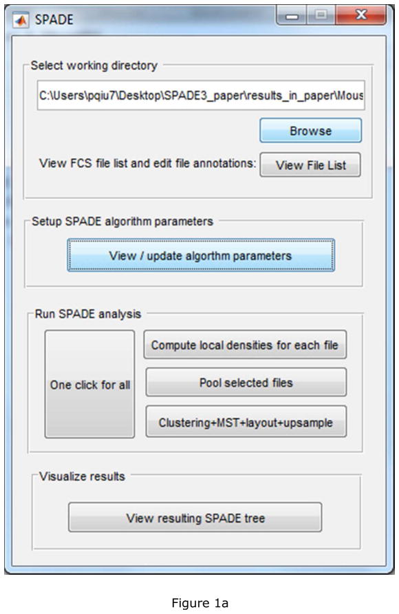
To showcase the algorithm improvements and software implementation, a mouse bone marrow dataset is analyzed. The data contains measurements of 8 protein markers on half a million cells, and the markers are able to delineate major cell subpopulations in mouse bone marrow. The data is available at http://pengqiu.gatech.edu/software/SPADE/data/mouseBM.fcs. Data stored in the fcs file is already compensated and transformed by hyperbolic inverse sine transformation. The software starts with the main control window shown in Figure 1(a). After the “Browse” button is used to select the directory that contains the FCS [37] data to be analyzed, another window will pop-up to display the list of recognized data files in the selected folder.

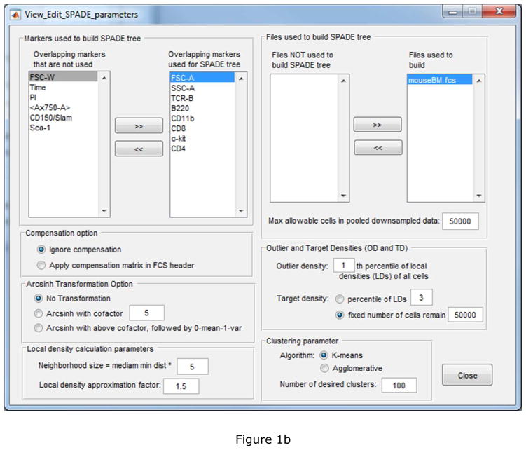
Figure 1.

Screenshots of the deterministic SPADE software: (a) main control window, (b) parameter setting window, and parameters used for the mouse bone marrow data.

Figure 1(b) shows the parameter setting interface for users to conveniently set and update parameters for SPADE analysis. (1) Typically, markers used to build the SPADE tree are markers that would have been used if one were to perform manual gating analysis. (2) By default, all data files are used to build the tree, unless the user would like to reserve some data files for validation and comparison. (3) For FCS data files generated by conventional flow cytometry, users should choose to apply compensation and hyperbolic inverse sine (arcsinh) transformation with cofactor of 150. For CyTOF data, the appropriate setting is to ignore compensation and arcsinh transformation with cofactor of 5. For data generated by other FCS file format converters, the appropriate setting depends on whether the raw data or the compensated data is store in the data files. (4) The default downsampling setting is to remove the bottom 1% outlier cells with the lowest local density, and downsample to 20000 cells for each data file separately. The target number of cells is typically less than $\frac{1}{10}$ of the number of cells in each data file. (5) When a large collection of data files are analyzed together, the total number of pooled downsampled cells can be extremely large, making the subsequent SPADE components computationally expensive and intractable. To guard against that, the maximum allowable cells parameter is defined. If the pooled downsampled data exceeds that parameter, SPADE performs another round of deterministic density-dependent downsampling to reduce the pooled downsampled data to the maximum allowed number of cells, and then proceeds to the subsequent components. (6) One key idea in SPADE is to over-cluster the data, so that the resulting tree is able to capture the underlying differentiation hierarchy among the cells. For high-content flow cytometry and CyTOF data, the number of desired clusters is typically around 100 ~ 300, much larger than the expected number of cell types in the data.

After setting the parameters as show in Figure 1(b), SPADE can be performed step-by-step by sequentially clicking the three buttons in the third section of the main control window. In addition, the one-click-for-all button conveniently performs the entire SPADE analysis pipeline. Run time of the analysis depends on the size of the data files. Typically, the density-dependent downsampling component is the most time consuming. For this mouse bone marrow dataset with 8 selected markers and 500,000 cells, deterministic density-dependent downsampling took roughly 20 minutes, whereas the rest of SPADE took less than 1 minute, on a PC desktop with Intel i7 CPU @ 3.40 GHz. This is approximately double the run time compared to the original SPADE algorithm. The run time increases linearly with respect to the number of markers, and between linearly and quadratically with respect to the number of cells, depending on how the cells are distributed.

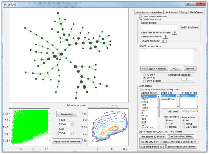
The bottom button in the main control window brings up Figure 2, a highly interactive visualization interface to display the SPADE tree. The tree can be colored by marker expression to visualize which parts of the tree are positive for what protein marker [4], or expression ratio across different samples for markers not used to build the tree [38], or cell frequency percentages to show distribution changes among different samples [10]. The default colorbar shows the range from 5th to 95th percentiles of the variation in the data, and the range can be manually adjusted.

Figure 2.

Screenshot of SPADE visualization interface.

Tree nodes can be selected and moved by mouse, allowing users to manually adjust the automatically generated layout of the tree. Cells belonging to the selected nodes can be highlighted in the biaxial plots, visualizing how the selected nodes would look like in conventional gating plots. Numerical indices of the selected nodes are listed next to the add-to-annotation button, which remembers the selected nodes and draws a bubble around them. This function enables users to manually annotate and interpret the SPADE tree using the software.

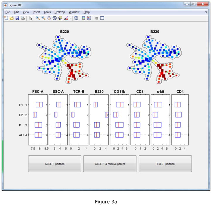
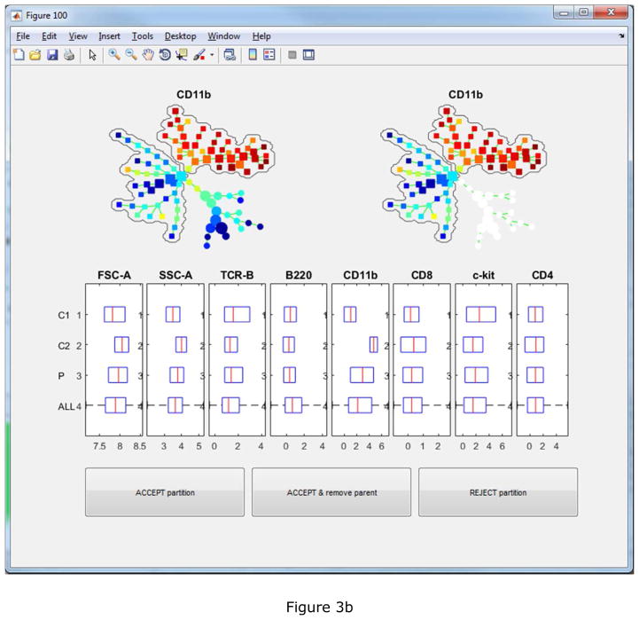
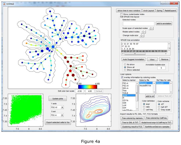
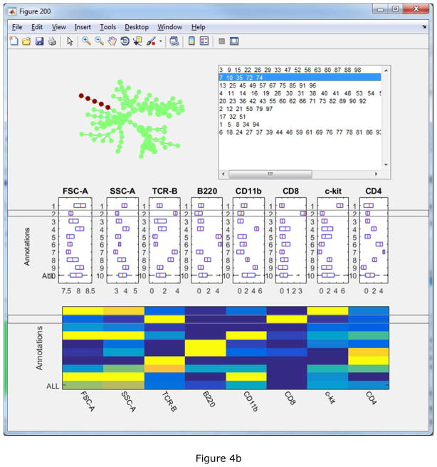
To facilitate the interpretation and annotation, the edge removal algorithm described above is implemented in the auto-suggest-annotation button. The algorithm will examine the mouse-selected region of the tree, or the entire tree if nothing is selected, and automatically suggest the best partitioning based on all markers used to build the tree. The reasons of the suggested partitioning are displayed in another window, where the users can choose to accept or reject it. In this example dataset, the first suggested partitioning is shown in Figure 3(a). The boxplots show that the two resulting pieces (“C1” and “C2”) differ in FSC-A, SSC-A, TCR-B and B220. “P” represents the combination of the two pieces and ”ALL” represents the entire tree. The SPADE trees is colored by B220, the marker that shows the strongest difference. Two bubbles are drawn to visualize the partitioning. When the second partitioning is suggested, the two SPADE tree visualizations will look different as shown in Figure 3(b). In the upper right tree, only nodes in the partitioned part of the tree are colored by CD11b, which contributes most to the second suggested partitioning. After eight rounds of the semi-automated annotation algorithm, the SPADE tree is partitioned into nine pieces, as shown in Figure 4(a) colored by average expression of B220 for each tree node. The boxplots and heatmap in Figure 4(b) summarizes the mean marker expressions across the annotations. For example, the heatmap shows that the second annotation is positive for TCR-B and CD8, indicating that the second annotation represents the CD8+ T cells. The fifth and sixth annotations are both positive for B220, but differ in CD4 expression, indicating that they represent B cells and dendritic cells respectively.

Figure 3.

The first two automated partitioning suggestions. Boxplots show which markers support the suggested partitioning. Bubbles are drawn to visualize the partitioning. The tree is colored by the marker that contributes the most to the suggestion. In the upper-left tree, all nodes are colored. In the upper-right tree, only nodes involved in the suggested partitioning are colored.

Figure 4.

Semi-automated partitioning result: (a) visualization interface displaying the partitioning, (b) interactive boxplot and heatmap summarizing the marker expression combination of the annotations.

In the bottom right section of the visualization interface, several functions are implemented to export SPADE results to formats useful for other analytical tools. The SPADE tree, and its colored and annotated versions, can be exported to PDF format to generate publication quality figures. The layout of the tree can be exported to GML format compatible with Cytoscape [39]. The mean marker expressions and percentage frequencies of the nodes and annotations can be exported into tab-delimited TXT files for statical analysis in MATLAB and R. The clustering results can be appended in to FCS files which can be visualized by FlowJo and other flow cytometry analysis software [37]. When multiple samples are analyzed jointly, the Earth Mover’s Distance (EMD) between each pair of samples is calculated, forming a distance matrix that can be used in machine learning analysis [10].

4 Discussion

The deterministic downsampling and clustering algorithms lead to deterministic SPADE. Compared to the original SPADE algorithm, deterministic SPADE should in most cases generate similar results. In the previous analysis of the above mouse bone marrow data, manual annotations of the original SPADE tree identified 7 cell populations that were highly consistent with manual gating [4]. The tree partitioning algorithm of deterministic SPADE generated 9 annotations. As shown in the bottom panel of Figure 4(b), the 3rd annotated population is negative for all markers. The 4th and 9th annotations represent myeloid cells with slightly different CD4 expression. The remaining 6 annotations capture the same populations as in the original analysis (c-kit+: 1st, B cells: 5th, Dendritic cells: 6th, T cell subtypes: 2nd 7th and 8th). Table 1 shows that the deterministic SPADE annotations are highly consistent with the manual gates in [4], and the level of consistency is similar to the original SPADE algorithm.

Table 1.

Comparison of deterministic SPADE and manual gating, expressed in terms of the number of overlapping cells between each manual gate and each annotated SPADE tree region.

		Manual gates
		B cell – 150,314	T cell – 14,699	CD4+ – 2,808	CD8+ – 6,055	Myeloid – 209,079	HSPC – 418
Annotated deterministic SPADE	B cell – 150,375	144,616 (96.2%)	8 (<0.1%)	0	0	2,286 (1.1%)	0
	Dendritic – 6,517	5,687 (3.8%)	0	0	0	282 (0.1%)	0
	T cell – 17,158	0	12,796 (87.1%)	2,806 (99.9%)	6,047 (99.9%)	2,435 (1.2%)	0
	CD4+ – 2,964	0	2,897 (19.7%)	2,791 (99.4%)	0	22 (<0.1%)	0
	CD8+ – 7,753	0	7,478 (50.9%)	0 6,040	(99.8%)	36 (<0.1%)	0
	Myeloid – 204,687	0	87 (0.6%)	0	0	202,300 (96.8%)	0
	c-kit+ – 17,924	7 (<0.1%)	852 (5.8%)	2 (<0.1%)	8 (<0.1%)	1,725 (0.8%)	402 (96.2%)

The total number of cells in each gate and each annotated region are listed. The percentages are defined as the ratio between the number of overlapping cells and the total number of cells in the corresponding manual gate, thereby representing the percent of cells in a gate that are assigned to each SPADE region. Large values in shaded entries indicate the consistency between manual gating and deterministic SPADE.

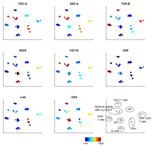
To evaluate the overall robustness of deterministic SPADE and automated annotation, 100 subsampled datasets were generated, each containing a random subset of 90% of the cells. Deterministic SPADE was applied to each dataset separately. For each resulting tree, 8 iterations of the tree partitioning algorithm were applied to generate 9 annotations, similar to the setting in Figure 4(a), and the centers of the annotations were computed. With the deterministic algorithms, the tree structure can still vary among the 100 analysis. However, the annotations are robust. Figure 5 shows the tSNE visualization of these 900 annotation centers, colored by various markers. The annotation centers form 9 groups, each corresponding to a distinct annotation in Figure 4(b). This result shows that the deterministic SPADE algorithm is able to generate robust biological interpretations, as well as the robustness of the tree partitioning algorithm.

Figure 5.

Robustness of deterministic SPADE and tree partitioning algorithms. 100 random subsamples of the mouse bone marrow dataset were analyzed, with 9 automatically generated annotations in each analysis. In the tSNE visualization, the centers of the 9*100 annotations formed 9 groups corresponding to distinct populations, which showed the robustness of the annotations.

The source code of the improved algorithm is provided for researchers who would like to build their own variation of the analysis pipeline, or build their own algorithms that can use certain components of SPADE. One such example is a combination of tSNE and SPADE, applying tSNE for dimension reduction and then SPADE for clustering and tree-based visualization [40]. The software is not designed to perform such a combination, but the source code can be rearranged to perform the analysis and generate result files that can be loaded into the SPADE software, for visualization and interpretation purposes. The software implementation and graphical user interface make it convenient to perform SPADE analysis, visualize and interact with the resulting tree, and connect to other analytic tools. Moreover, the semi-automated annotation algorithm significantly reduces the time and effort required for biological interpretation of the SPADE analysis.

References

- 1.Perfetto SP, Chattopadhyay PK, Roederer M. Seventeen-colour flow cytometry: unravelling the immune system. Nat Rev Immunol. 2004;4:648–655. doi: 10.1038/nri1416. [DOI] [PubMed] [Google Scholar]
- 2.Chattopadhyay PK, Hogerkorp CM, Roederer M. A chromatic explosion: the development and future of multiparameter flow cytometry. Immunology. 2008;125:441–449. doi: 10.1111/j.1365-2567.2008.02989.x. [DOI] [PMC free article] [PubMed] [Google Scholar]
- 3.Lu Y, Xue Q, Eisele MR, Sulistijo ES, Brower K, et al. Highly multiplexed profiling of single-cell effector functions reveals deep functional heterogeneity in response to pathogenic ligands. Proceedings of the National Academy of Sciences. 2015;112:E607–E615. doi: 10.1073/pnas.1416756112. [DOI] [PMC free article] [PubMed] [Google Scholar]
- 4.Qiu P, Simonds E, Bendall S, Gibbs K, Jr, Bruggner R, et al. Extracting a cellular hierarchy from high-dimensional cytometry data with SPADE. Nature Biotechnology. 2011;29:886–891. doi: 10.1038/nbt.1991. [DOI] [PMC free article] [PubMed] [Google Scholar]
- 5.Singh S, Clarke I, Terasaki M, Bonn V, Hawkins C, et al. Identification of a cancer stem cell in human brain tumors. Cancer Res. 2003;63:5821–8. [PubMed] [Google Scholar]
- 6.Bursch LS, Wang L, Igyarto B, Kissenpfennig A, Malissen B, et al. Identification of a novel population of langerin+ dendritic cells. The Journal of experimental medicine. 2007;204:3147–3156. doi: 10.1084/jem.20071966. [DOI] [PMC free article] [PubMed] [Google Scholar]
- 7.Betts M, Brenchley J, Price D, De Rosa S, Douek D, et al. Sensitive and viable identification of antigen-specific cd8+ t cells by a flow cytometric assay for degranulation. J Immunol Methods. 2003;281:65–78. doi: 10.1016/s0022-1759(03)00265-5. [DOI] [PubMed] [Google Scholar]
- 8.Qiu P. Computational prediction of manually gated rare cells in flow cytometry data. Cytometry Part A. 2015;87:594–602. doi: 10.1002/cyto.a.22654. [DOI] [PMC free article] [PubMed] [Google Scholar]
- 9.Irish JM, Myklebust JH, Alizadeh AA, Houot R, Sharman JP, et al. B-cell signaling networks reveal a negative prognostic human lymphoma cell subset that emerges during tumor progression. Proceedings of the National Academy of Sciences. 2010;107:12747–12754. doi: 10.1073/pnas.1002057107. [DOI] [PMC free article] [PubMed] [Google Scholar]
- 10.Qiu P. Inferring phenotypic properties from single-cell characteristics. PLoS One. 2012;7:e37038. doi: 10.1371/journal.pone.0037038. [DOI] [PMC free article] [PubMed] [Google Scholar]
- 11.Chattopadhyay P, Price D, Harper T, Betts M, Yu J, et al. Quantum dot semiconductor nanocrystals for immunophenotyping by polychromatic flow cytometry. Nature Medicine. 2006;12:972–977. doi: 10.1038/nm1371. [DOI] [PubMed] [Google Scholar]
- 12.Bendall SC, Nolan GP, Roederer M, Chattopadhyay PK. A deep profiler’s guide to cytometry. Trends in immunology. 2012;33:323–332. doi: 10.1016/j.it.2012.02.010. [DOI] [PMC free article] [PubMed] [Google Scholar]
- 13.Herzenberg L, Tung J, Moore W, Herzenberg L, Parks D. Interpreting flow cytometry data: a guide for the perplexed. Nature Immunology. 2006;7:681–685. doi: 10.1038/ni0706-681. [DOI] [PubMed] [Google Scholar]
- 14.Maecker HT, Rinfret A, D’Souza P, Darden J, Roig E, et al. Standardization of cytokine flow cytometry assays. BMC Immunol. 2005;6:13. doi: 10.1186/1471-2172-6-13. [DOI] [PMC free article] [PubMed] [Google Scholar]
- 15.Murphy RF. Automated identification of subpopulations in flow cytometric list mode data using cluster analysis. Cytometry. 1985;6:302–309. doi: 10.1002/cyto.990060405. [DOI] [PubMed] [Google Scholar]
- 16.Aghaeepour N, Nikolic R, Hoos H, RRB Rapid cell population identification in flow cytometry data. Cytometry A. 2011;79:6–13. doi: 10.1002/cyto.a.21007. [DOI] [PMC free article] [PubMed] [Google Scholar]
- 17.Ge Y, Sealfon S. flowPeaks: a fast unsupervised clustering for flow cytometry data via K-means and density peak finding. Bioinformatics. 2012 doi: 10.1093/bioinformatics/bts300. Epub. [DOI] [PMC free article] [PubMed] [Google Scholar]
- 18.Lo K, Brinkman R, Gottardo R. Automated gating of flow cytometry data via robust model-based clustering. Cytometry A. 2008;73:321–332. doi: 10.1002/cyto.a.20531. [DOI] [PubMed] [Google Scholar]
- 19.Boedigheimer M, Ferbas J. Mixture modeling approach to flow cytometry data. Cytometry A. 2008;73:421–429. doi: 10.1002/cyto.a.20553. [DOI] [PubMed] [Google Scholar]
- 20.Chan C, Feng F, Ottinger J, Foster D, West M, et al. Statistical mixture modeling for cell subtype identification in flow cytometry. Cytometry A. 2008;73:693–701. doi: 10.1002/cyto.a.20583. [DOI] [PMC free article] [PubMed] [Google Scholar]
- 21.Pyne S, Hu X, Kang K, Rossin E, Lin T, et al. Automated high-dimensional flow cytometric data anlysis. Proceedings of the National Academy of Science. 2009;106:8519–8524. doi: 10.1073/pnas.0903028106. [DOI] [PMC free article] [PubMed] [Google Scholar]
- 22.Walther G, Zimmerman N, Moore W, Parks D, Meehan S, et al. Automatic clustering of flow cytometry data with density-based merging. Advances in Bioinformatics. 2009 doi: 10.1155/2009/686759. [DOI] [PMC free article] [PubMed] [Google Scholar]
- 23.Qian Y, Wei C, Lee F, Campbell J, Halliley J, et al. Elucidation of seventeen human peripheral blood B-cell subsets and quantification of the tetanus response using a density-based method for the automated identification of cell populations in multidimensional flow cytometry data. Cytometry Part B: Clinical Cytometry. 2010;78B:S69–S82. doi: 10.1002/cyto.b.20554. [DOI] [PMC free article] [PubMed] [Google Scholar]
- 24.Naumann U, Luta G, Wand M. The curvhdr method for gating flow cytometry samples. BMC Bioinformatics. 2010:11. doi: 10.1186/1471-2105-11-44. [DOI] [PMC free article] [PubMed] [Google Scholar]
- 25.Sugar I, Sealfon S. Misty mountain clustering: application to fast unsupervised flow cytometry gating. BMC Bioinformatics. 2010:11. doi: 10.1186/1471-2105-11-502. [DOI] [PMC free article] [PubMed] [Google Scholar]
- 26.Naim I, Datta S, Rebhahn J, Cavenaugh J, Mosmann T, et al. Swift-scalable clustering for automated identification of rare cell populations in large, high-dimensional flow cytometry datasets, part 1: algorithm design. Cytometry A. 2014;85:408–21. doi: 10.1002/cyto.a.22446. [DOI] [PMC free article] [PubMed] [Google Scholar]
- 27.Mosmann T, Naim I, Rebhahn J, Datta S, Cavenaugh J, et al. Swift-scalable clustering for automated identification of rare cell populations in large, high-dimensional flow cytometry datasets, part 2: biological evaluation. Cytometry A. 2014;85:422–33. doi: 10.1002/cyto.a.22445. [DOI] [PMC free article] [PubMed] [Google Scholar]
- 28.Zare H, Shooshtari P, Gupta A, Brinkman R. Data reduction for spectral clustering to analyze high throughput flow cytometry data. BMC Bioinformatics. 2010;11:403. doi: 10.1186/1471-2105-11-403. [DOI] [PMC free article] [PubMed] [Google Scholar]
- 29.Cron A, Gouttefangeas C, Frelinger J, Lin L, Singh S, et al. Hierarchical modeling for rare event detection and cell subset alignment across flow cytometry samples. PLoS Comput Biol. 2013;9:e1003130. doi: 10.1371/journal.pcbi.1003130. [DOI] [PMC free article] [PubMed] [Google Scholar]
- 30.Aghaeepour N, Finak G, Hoos H, et al. FlowCAP Consortium, DREAM Consortium. Critical assessment of automated flow cytometry data analysis techniques. Nature methods. 2013;10:228–238. doi: 10.1038/nmeth.2365. [DOI] [PMC free article] [PubMed] [Google Scholar]
- 31.Van der Maaten L, Hinton G. Visualizing data using t-sne. Journal of Machine Learning Research. 2008;9:85. [Google Scholar]
- 32.Amir eA, Davis K, Tadmor M, Simonds E, Levine J, et al. viSNE enables visualization of high dimensional single-cell data and reveals phenotypic heterogeneity of leukemia. Nat Biotechnol. 2013;31:545–52. doi: 10.1038/nbt.2594. [DOI] [PMC free article] [PubMed] [Google Scholar]
- 33.Su T, Dy J. A deterministic method for initializing k-means clustering. Tools with Artificial Intelligence, 2004. ICTAI 2004. 16th IEEE International Conference on; IEEE; 2004. pp. 784–786. [Google Scholar]
- 34.Linderman MD, Bjornson Z, Simonds EF, Qiu P, Bruggner RV, et al. Cytospade: high-performance analysis and visualization of high-dimensional cytometry data. Bioinformatics. 2012;28:2400–2401. doi: 10.1093/bioinformatics/bts425. [DOI] [PMC free article] [PubMed] [Google Scholar]
- 35.Kotecha N, Krutzik PO, Irish JM. Web-based analysis and publication of flow cytometry experiments. Curr Protoc Cytom. 2010;53:1–10. doi: 10.1002/0471142956.cy1017s53. [DOI] [PMC free article] [PubMed] [Google Scholar]
- 36.Graham RL, Hell P. On the history of the minimum spanning tree problem. Annals of the History of Computing. 1985;7:43–57. [Google Scholar]
- 37.Seamer L, Bagwell C, Barden L, Redelman D, Salzman G, et al. Proposed new data file standard for flow cytometry, version fcs 3.0. Cytometry. 1997;28:118–22. doi: 10.1002/(sici)1097-0320(19970601)28:2<118::aid-cyto3>3.0.co;2-b. [DOI] [PubMed] [Google Scholar]
- 38.Bendall S, Simonds E, Qiu P, Amir E, Krutzik P, et al. Single cell mass cytometry of differential immune and drug responses across the human hematopoietic continuum. Science. 2011;332:687–696. doi: 10.1126/science.1198704. [DOI] [PMC free article] [PubMed] [Google Scholar]
- 39.Shannon P, Markiel A, Ozier O, Baliga N, Wang J, et al. Cytoscape: a software environment for integrated models of biomolecular interaction networks. Genome research. 2003;13:2498–2504. doi: 10.1101/gr.1239303. [DOI] [PMC free article] [PubMed] [Google Scholar]
- 40.Diggins KE, Ferrell PB, Irish JM. Methods for discovery and characterization of cell subsets in high dimensional mass cytometry data. Methods. 2015;82:55–63. doi: 10.1016/j.ymeth.2015.05.008. [DOI] [PMC free article] [PubMed] [Google Scholar]