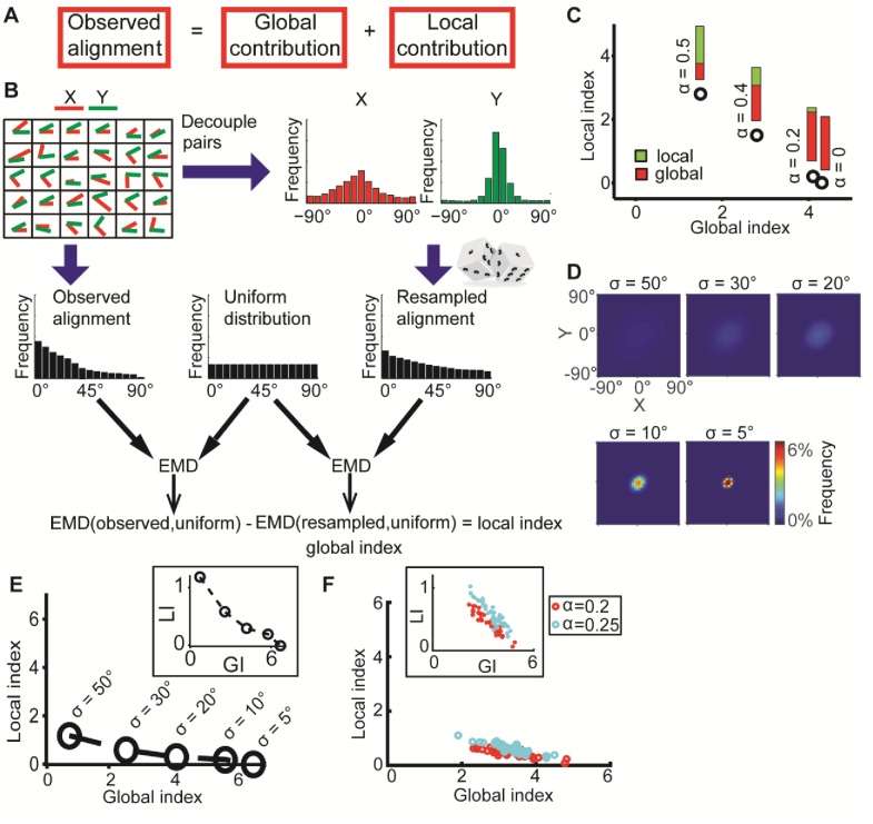
Figure 2. DeBias algorithm.

(A) Underlying assumption: the observed relation between two variables is a cumulative process of a global bias and a local interaction component. (B) Quantifying local and global indices: sample from the marginal distributions X, Y to construct the resampled distribution. The global index (GI) is calculated as the Earth Movers Distance (EMD) between the uniform and the resampled distributions. The local index (LI) is calculated as the subtraction of the GI from the EMD between the uniform and the observed distribution. (C) Local and global indices calculated for the examples from Figure 1C. Black circles represent the (GI,LI) value for the corresponding example in Figure 1C, bars represent the relative contribution of the local (green) and global (red) index to the observed alignment. (D-E) Simulation using a constant interaction parameter α = 0.2 and varying standard deviations of X, Y, σ = 50° to 5°. (D) Joint distributions. Correlation between X and Y is (subjectively) becoming less obvious for increasing global bias (decreasing σ). (E) GI and LI are negatively correlated: decreased σ enhances GI and reduces LI. The change in GI is ~4 fold larger compared to the change in LI indicating that the GI has a limited effect on LI values. Inset: stretched LI emphasizes the negative correlation. (F) Both LI and GI are needed to discriminate between simulations with different interaction parameters. α = 0.2 (red) or 0.25 (cyan), σ is drawn from a normal distribution (mean = 25°, standard deviation = 4°). Number of simulations = 40, for each parameter setting. Inset: stretched LI emphasizes the discrimination. Number of histogram bins, K = 15, for all simulations.

DOI: http://dx.doi.org/10.7554/eLife.22323.004

Figure 2—figure supplement 1. Simulations demonstrating the negative local interactions induce negative local indices.

Simulations were performed as in Figure 1B: X, Y truncated normal distributions with mean 0 and σ = σ_X = σ_Y; ζ = αθ, but with α < 0 as the negative interaction. Shown are GI and LI values for four simulations with increased global bias (i.e., smaller standard deviation σ_X, σ_Y) and increased negative local interaction (left-to-right), all scenarios have similar observed mean alignment of ~19° (corresponding to the simulations in Figure 1C). 

DOI: http://dx.doi.org/10.7554/eLife.22323.005