Dynamic cellular finite-element method for modelling large-scale cell migration and proliferation under the control of mechanical and biochemical cues: a study of re-epithelialization

Abstract

Computational modelling of cells can reveal insight into the mechanisms of the important processes of tissue development. However, current cell models have limitations and are challenged to model detailed changes in cellular shapes and physical mechanics when thousands of migrating and interacting cells need to be modelled. Here we describe a novel dynamic cellular finite-element model (DyCelFEM), which accounts for changes in cellular shapes and mechanics. It also models the full range of cell motion, from movements of individual cells to collective cell migrations. The transmission of mechanical forces regulated by intercellular adhesions and their ruptures are also accounted for. Intra-cellular protein signalling networks controlling cell behaviours are embedded in individual cells. We employ DyCelFEM to examine specific effects of biochemical and mechanical cues in regulating cell migration and proliferation, and in controlling tissue patterning using a simplified re-epithelialization model of wound tissue. Our results suggest that biochemical cues are better at guiding cell migration with improved directionality and persistence, while mechanical cues are better at coordinating collective cell migration. Overall, DyCelFEM can be used to study developmental processes when a large population of migrating cells under mechanical and biochemical controls experience complex changes in cell shapes and mechanics.

1. Introduction

Cells are the basic functional elements of living bodies. Cell–cell and cell–environment interactions largely maintain biological tissues [1]. Many experiments have been performed to understand the mechanisms behind cellular interactions, cell behaviours and tissue patterning [2]. However, many subcellular processes such as cytoskeleton generated physical forces and cell–cell transmitted mechanical forces are difficult to access experimentally [3]. Computational modelling of cell–cell and cell–environment interactions, therefore, provide useful means of investigations that complement experimental studies to answer questions such as how cellular border forces between cell and environment control the closure of epithelial gaps [3], and how cell shape influences the field of traction force [4].

A number of computational cell models have been developed [5–18]. These models can be broadly categorized into continuum and discrete models. Continuum models are based on differential equations to model the spatial–temporal changes of protein density in cells, and changes of cell populations in a tissue. In these models, individual cells and interactions are not considered explicitly [5–7]. Discrete models such as the cellular Potts model [8–10], vertex model [11,12,19–21], centric model [13], subcellular element model [14], immersed boundary model [15] and finite-element model [16,17] are based on discretized elementary units to model cell morphology and motility. These models can describe cell shape and intercellular interactions explicitly. However, there are many limitations. The cellular Potts model represents each cell as a set of lattice sites [22]. The underlying physical forces and cellular mechanics are difficult to recover from spatial changes of lattice sites. The vertex model describes the changes in cell shape based on minimizing energy under forces acting on cell boundary junctions [11]. The specific cell shape contributing to the mechanical energy of cell interior is usually not considered [11]. The centric model can only describe the shape of a cell as one or two simple spheres [13]. The subcellular element model can describe cell shape in high resolution. However, the distances between intra/intercellular elements are artificially maintained through an arbitrarily imposed Morse potential [14], which is not physically realistic [23]. The immersed boundary model can also describe cell shapes in detail. However, the physical boundary of the cell body may not fully conform to the grid underneath [24], which lead to irregular boundary points in the solution. The finite-element cell model can describe both cell shape and cell mechanics accurately [16,25]. However, this method permits only limited changes in cell shape and allows limited flexibility of cell movement, and therefore is restricted to cellular and tissue processes that do not involve free movement of individual cells. Owing to these limitations, accurate modelling of physiological processes involving large scale and collective cell migration at a detailed cellular level remains a challenging task.

Here we describe a novel dynamic cellular finite-element model (DyCelFEM), which has a number of advantages over existing discrete cell models. It can accurately describe the full span of cell movement, from the free movement of individual cells to large scale collective cell migration. In addition, changes in shapes of moving cells under the control of cell mechanics are fully accounted for. Furthermore, the transmission of mechanical force regulated by intercellular adhesion and its rupture are also explicitly modelled. As biochemical signals strongly influence cell behaviour and tissue patterning [26], intracellular networks of protein signalling are also embedded inside individual cells in our model. Our DyCelFEM model is therefore suited to study biological processes involving large-scale collective cell motion under the regulation of biochemical signals and mechanical forces, with accurate description of cell shapes and cell mechanics.

In this study, we apply DyCelFEM to investigate the effects of biochemical and mechanical cues on migration and proliferation of a population of keratinocyte cells and on tissue patterning using a simplified re-epithelialization model of wound tissue. We examine the directionality and persistence of cell migration, and cell–cell coordination during re-epithelialization under different guidance control mechanisms of cell migration. Our results suggest that the influence of biochemical cues are restricted to areas close to the wound bed, while mechanical cues influence the tissue globally. Furthermore, biochemical cues are better at guiding cell migration with improved directionality and persistence, while mechanical cues are better at coordinating collective cell migration. These findings provide useful information towards understanding the full mechanism of wound healing.

2. Model and methods

2.1. Geometry, discretization, deformation energy and dynamic changes of cells

2.1.1. Geometry and discretization of the cell

In our model, a two-dimensional cell Ω is defined by its boundary ∂Ω, which is represented by an oriented polygon connecting a set of boundary vertices V_∂Ω ≡{v_i ∈ ∂Ω ⊂ ℝ²}. The cell boundary ∂Ω is a closed chain of oriented edges (e_1,2, e_2,3, … , e_n,1), where edge e_i,i+1 connects modulus n consecutive boundary vertices v_i and v_i+1 in the anticlockwise orientation. We denote the location of a vertex v_i as x_i. We first compute the Delaunay triangulation D_Ω of the cell Ω using only boundary vertices V_∂Ω. We then test if the radius of the circumsphere of any triangle in D_Ω is larger than a threshold. If so, a new vertex is inserted at the circumcenter of this triangle and D_Ω is updated accordingly [27]. This is repeated until all new triangles have their circumsphere radius smaller than a threshold. The cell Ω is therefore represented by a simplicial complex K_Ω, composed of a set of boundary vertices and inserted interior vertices V_Ω = V_∂Ω ∪V_Int, a set of edges E_Ω = {e_{i, j} | v_i, v_j ∈ V_Ω} and a set of triangles T_Ω = {τ_{i, j, k} | v_i, v_j, v_k ∈ V_Ω} (figure 1a,b; see more details on in the electronic supplementary material, text S1).

Figure 1.

Geometry, discretization and dynamic changes of cells. (a) The boundary of each cell is defined by a anticlockwise oriented polygon containing a number of boundary vertices. (b) Triangular mesh tiling up each cell. (c) Cell growth from time t to t + Δt. The displacement vector Δv_i of vertex v_i after cell growth with given incremental cell volume Δ|Ω| can be obtained by solving equations (2.3) and (2.6) that relates Δv_i to Δ|Ω| through the Jacobian determinant. (d) When the volume of a cell Ω is doubled, cell proliferation occurs and it is then divided into two daughter cells Ω₁ and Ω₂ along the shortest axis of Ω. (e) Cell migration from time t to t + Δt. The protrusion force driving cell migration on each boundary vertex v_i on the leading edge is calculated, where f_af is the parameter of protrusion force from t to t + Δt. (f) Contraction forces (in red) resulting from cell elasticity are generated in response to the protrusion force on the leading edges. The attached vertices in adhesion linkage v_1,i and v_2,j (in green) from two cells in contact with one another are separated if the contraction force generated is larger than the threshold of adhesion rupture force. The purple and light green triangles are triangular elements to build sub-stiffness matrices for v_1,i and v_2,j, respectively, to recover the contraction force.

2.1.2. Deformation energy of the cell

We use u(x) to represent the deformation vector of the cell at x, strain tensor ε(x) to describe the local deformation at x and the stress tensor σ to represent the forces at x. During cell motility, we assume that the recovery of cell shape is incomplete due to the plastic deformation originating from bond ruptures within the cytoskeleton as shown in [28]. For simplicity, we assume cell is linearly elastic during each time step and is plastic between time steps. Therefore, we re-calculate the triangular mesh T_Ω for each cell Ω after each time step and reset the stress to zero after location update (see discussion on the reason that viscoelasticity can be neglected in electronic supplementary material, text S1).

The overall free energy E_Ω of cell Ω is given by the sum of elastic energy E_el, contractile energy E_co, adhesion energy E_ad and force energy E_f.

The elastic energy takes the form . The contractile energy arising from the contractility of the cell takes the form , where σ_a is a homogeneous contractile pressure resulting from active bulk process [4]. Using Gauss' divergence theorem, it can be further written as .

The adhesion between the cell and substratum contributes to the total energy of the cell. We follow [4] and assume that the adhesion force F_a generated from the substratum on the cell is proportional to the displacement u according to Hooke's Law of F_a = Yu. The L₂ norm of the displacement field gives the adhesion energy E_a as , where Y is a constant parameter proportional to the stiffness of substratum and to the strength of focal adhesion between cell and the substratum [4].

The boundary adhesion energy between neighbouring cells is proportional to the size of the contacting surfaces following [29]. Specifically, the adhesion energy between a cell Ω and the set of its neighbouring cells {Ω_i} takes the form of , where n(x) is the surface normal vector at x, and f_a is a constant adhesion force per unit length along the cell–cell boundary. This constant adhesion force occurs when the adhesive contact is formed on the cell–cell boundary and disappears when the adhesive contact is removed from the cell–cell boundary. Therefore, adhesion strength between cells depends on the geometry of the cell–cell boundary.

The force energy E_f due to the growth forces f_g(x) and protrusive migration force f_m(x) occurring in Ω can be written as . Therefore, the overall free energy E_Ω of the cell Ω can be written as

2.1

The deformed cell reaches its balance state when the strain energy of the cell E_Ω reaches a minimum, at which we have ∂E_Ω(u)/∂u = 0.

For each triangular element τ_i,j,k ∈ T_Ω of Ω, equation (2.1) can be written using the stiffness matrix method as a linear equation

where K_τ is the stiffness matrix of τ_i,j,k, u_τ is the displacement of τ_i,j,k and f_τ is the integrated force vector on τ_i,j,k (see electronic supplementary material, S1 for details of the derivation).

We then gather the element stiffness matrices of all triangular meshes in all cells and assemble them into a global stiffness matrix K. The adhesion energy term in equation (2.2) contributes to K by adding a scaled identity matrix, which prevents the system of equation (2.2) from being singular. The linear relationship between the concatenated vector u of all vertices of the cells and the external force vector f on all vertices is then given by

2.2

The behaviour of the whole collection of cells in the stationary state at a specific time step can then be obtained by solving this non-singular linear equation. For vertex v_i at x_i, its new location is then updated as x_i′ = x_i + u(v_i). As migrating cells rapidly reconstruct their cytoskeleton and adhesive structures [30], we re-calculate the triangle mesh T_Ω for each cell Ω and reset the stress to zero after location update. In our model, the time step Δt is fixed as 30 min (see electronic supplementary material, text S7 for discussion on the size of the time step).

2.1.3. Dynamic changes in cell geometry during cell growth, proliferation and migration

While the cell is moving, the positions of discretized vertices of cells change with time. We distribute forces driving cell motion onto the vertices of cells. The displacement vectors of the vertices can then be obtained by solving equation (2.2).

Cell growth. At each time interval, we consider an idealized growth force f_g that would drive a cell Ω to grow by an incremental volume Δ|Ω|, in the absence of its neighbouring cells. We assume that the direction of the growth force f_g,i at the boundary vertex v_i is along the direction of the normal vector n_i at v_i. We also assume that the strength |f_g,i| is proportional to the length of edges associated with v_i and is

2.3

where γ is a scalar. We then calculate γ by relating the volume change Δ|Ω| and the displacement vectors u(x) at locations x through the Jacobian determinant , where F(x) is the deformation gradient. We have

2.4

where I is the identity matrix. ∂u(x)/∂x for x ∈ τ_i,j,k can be interpolated as and , where b_i = x_j,2 − x_k,2 and c_i = x_j,1 − x_k,1 (see the electronic supplementary material for details). Equation (2.4) then can be written as:

2.5

As the displacement vectors u_g = {u₁, … ,u_n} of vertices in cell Ω are determined by u_g = K⁻¹_gf_g, where K_g is the stiffness matrix of Ω given by the geometry of the cell, combined with the scaled identity matrix incorporating the adhesion between the cell and the substrate and f_g is the integrated force vector of f_g,i given by equation (2.3). Then equation (2.5) can be rewritten as

2.6

Then the growth force f_g that gives the incremental volume change Δ|Ω| can be obtained by solving the coupled equations (2.3) and (2.6).

Cell proliferation. Cell proliferation occurs when the volume of the mother cell Ω is doubled. We divide Ω into two daughter cells Ω₁ and Ω₂ by adding a set of paired vertices along the shortest axis of Ω (figure 1c, between diagonal paired vertices).

Cell migration. To model cell migration, we distribute the protrusive migration forces f_m onto the vertices of the leading edges. Here leading edges are edges whose outward normal n and the unit vector of migration direction ν has the positive inner product: n · ν > 0. For each boundary vertex v_i on a leading edge, the protrusive migration force f_m,i driving v_i to migrate is calculated as

2.7

where f_af is the parameter of protrusion force per unit length, e_i−1,i and e_i,i+1 are edges connected to v_i (figure 1e).

2.2. Cell–cell adhesion and its rupture

Here we implicitly model cell–cell adhesions as adhesion linkages between two attached vertices from two neighbouring cells. Cell–cell adhesion occurs if the bodies of two cells would otherwise overlap. The attachment of adhesion linkage is added to each pair of vertices on the contacting surfaces, and the overlap is repaired by the Cell-merge primitive. The adhesion linkage then generates adhesion force f_a on the pair of attached vertices as shown in equation (2.1). In response to the protrusive migration force on the leading edges of a migrating cell, elastic force in the opposite direction occurs at the rear edges of the cell, which arises strictly from cell elasticity in our model. Once this elastic force exerted on an adhesive linkage between two vertices on two contacting cells surpasses a threshold f_θ of rupture force, the adhesion linkage between these vertices is severed.

We compute this elastic force at each vertex in the contacting surface of a cell with its neighbours in response to cell motion. For vertex v_1,i from cell Ω₁ on the contacting surface with cell Ω₂, we can recover this elastic force vector using the sub-stiffness matrix associated with v_1,i (figure 1f):

2.8

where K_1,i is the sub-stiffness matrix constructed using the set of triangles, namely, T_v1,i≡∪_v1,i∈τkτ_k, where each triangle τ_k ∈ Ω₁ contains vertex v_1,i (purple triangles in figure 1f). Here u_1,i is the displacement vector, which includes the displacement of vertex v_1,i and displacements of all of its surrounding vertices contained in T_v1,i. Currently, we do not consider additional active contractile processes when calculating forces for cell rupture. Therefore, u_1,i here is calculated using an adapted free energy excluding the contractile energy . For vertex v_2,j on cell Ω₂ attached to Ω₁, we recover the elastic force similarly. If , where n_1,i and n_2,j are unit normal vectors of v_1,i and v_2,j, we eliminate the attachment of adhesion linkage between vertices v_1,i and v_2,j (figure 1f). Here f_θ is the rupture force threshold per unit length, l is the half-length of the shared edge(s) between v_1,i and v_2,j.

2.3. Primitives for topologic and geometric changes

Here we use five primitives to model topologic and geometric changes for cells undergoing movement:

• — P1. Cell-merge: The intersecting surfaces of two colliding cells are identified and then replaced by contacting surfaces. Cell–cell adhesion is then added to each pair of attached vertices on the contacting surfaces (figure 2a).

• — P2. Cell-separation: The kinematic attachment of an adhesion linkage between a pair of attached vertices is then removed when it experiences contraction force larger than the threshold (figure 2b).

• — P3. Edge-subdivision: An edge longer than the threshold is then subdivided into two edges (figure 2c).

• — P4. Edge-simplification: An edge shorter than the threshold is then removed (figure 2d).

• — P5. Sliver-removal: A skinny triangle with an angle smaller than the threshold appears is then removed (figure 2e).

Figure 2.

Primitives for cell geometric and topologic changes. (a) P1. Cell-merge: The overlapping surfaces (red vertices) of the two colliding cells are detected by examining the intersection of their bounding boxes and then repaired. (b) P2. Cell-separation: previously attached vertices on the contact surfaces of two different cells are separated from each other. (c) P3. Edge-subdivision: an edge longer than the threshold is subdivided into two edges. (d) P4. Edge-simplification: an edge shorter than the threshold is removed. (e) P5. Sliver-removal: a skinny triangle with an angle smaller than the threshold is removed.

These primitives can exhaust all possible topologic changes of cells. In addition to the cell topologic change, it is also important to detect collisions of colliding cells. Details on implementation of collision detection and realization of topologic change using these primitives can be found in electronic supplementary material, text S2.

2.4. Model of wound tissue and re-epithelialization

2.4.1. Geometry of wound bed and tissue regions

We use a simplified wound tissue to study the re-epithelialization process (figure 3a). In our model, wound tissue is composed of keratinocyte cells and wound elements. The wound elements include both fibrin clots and fibroblasts, with the elastic property of the wound element determined mostly by the fibrin clot, the major component of the wound site [31] (see electronic supplementary material, table S2 for the parameter values of cell and element elasticity). The combination of all wound elements is called the wound bed. The wound bed size is set to 800 × 300 μm (figure 3a) in our model. We follow a previous study [32] and divide the locations of keratinocytes into four regions according to their distance to the wound edge: Regions I, II, III, and IV have distance 0–80 μm, 80–160 μm, 160–240 μm and greater than 240 μm to the wound edge, respectively (figure 3a). Results reported here were obtained using this model wound tissue consisting of 8741/929 cells/wound elements and 3 × 10⁵ vertices at the end of simulation. With a Pentium Dual CPU of 1.60 GHz and 4.00 GB RAM, each time step can be simulated in about 12 s.

Figure 3.

Model of wound tissue and re-epithelialization. (a) Top view of the skin wound tissue. Blue: keratinocytes; green: wound element. The size of the wound bed: 800 × 300 μm. The locations of keratinocytes are divided into four regions according to their distances to the wound edge: Regions I: 0–80 μm, II: 80–160 μm, III: 160–240 μm and IV: greater 240 μm. (b) Schematic of the intracellular signalling network. The synthesis and regulation relationship between the cell elements and the growth factors are represented by arrows. Detailed relationships are listed in electronic supplementary material, table S1. (c) In chemokinesis, the growth factor gradient (blue arrow) activates cell migration but cells move in random directions (green arrow). In chemotaxis, the migration direction is taken as the largest growth factor gradient (brown arrow), plus a random deviating angle sampled from the normal distribution of of angles (yellow arrow). (d) In cohesotaxis, a cell migrates along the direction of the vectors of local intercellular elastic force. The elastic force vectors (red arrows) on each vertex (red vertices) of the cell boundary with a neighbouring cell are summed, and the overall vector (orange arrow), plus a random deviating vector whose angle is sampled from the normal distribution of angles (purple arrow), gives the migration direction. (e) Wound closure ratio r(t_N) is given by the number of remaining discrete wound element units in the wound bed at time t_N divided by the total number of discrete wound element units before re-epithelialization. (f) Migration direction angle α(t_n) is the angle between the direction of migration (yellow arrow) and the direction of the cell to the nearest wound edge (red arrow). (g) Migration persistence p(t_N) is the ratio of the distance from the current position of the cell at time t_N to its original position (red line segment), divided by the length of the traversed path (yellow curve). (h) Normalized pair separation distance d_i,j(t_N) is the separation distance between a pair of cells at time t_N which were initially neighbours (orange line), normalized by the average length of cell traversed path (yellow curve).

2.4.2. Intracellular signalling network

During the re-epithelialization process, keratinocyte proliferation and migration are known to be controlled by an intracellular signalling network [26]. We use a simplified network taken from Menon et al. [33] (figure 3b) involving three growth factors, namely, keratinocyte growth factor (KGF), epidermal growth factor (EGF) and the transforming growth factor-β (TGF-β), which are known to be the most important growth factors for the re-epithelialization process [26] (see electronic supplementary material, table S1 for details).

Diffusion, synthesis and degradation of growth factors. Following Menon et al. [33], the change in local concentration y_i of a growth factor i is determined by its diffusion, synthesis and degradation:

2.9

where D_i is the diffusion coefficient of y_i, λ_s,i is the synthesis rate of y_i and λ_d,i is its degradation rate (see electronic supplementary material, table S2 for coefficient values). Details of the discretization of the diffusion equation can be found in our model in electronic supplementary material, text S3.

2.4.3. Cell behaviours during re-epithelialization

In our simplified model, keratinocytes can proliferate, migrate, apoptosize or become quiescent. This is controlled by a minimalistic network consisting of three growth factors (KGF, EGF and TGF-β, figure 3b). At a particular time step, the ith behaviour is stochastically chosen with probability

2.10

where i = 1,2,3 and 4 stands for proliferation, migration, apoptosis and quiescence, respectively. Following Menon et al. [33], the value of B₁ for proliferation is set to B₁ = α₁((1 + β_1,EGFd_EGF)(1 + β_1,KGFd_KGF)/(1 + β_1,TGF−βd_TGFβ)), where α₁ is a scaling factor, β_1,j is the coefficient for factor j, and d_j is its concentration density. The value of B₂ for migration is set to B₂ = α₂(1 + β_1,EGFd_EGF). We also set B₃ = α₃ for apoptosis and B₄ = α₄ for quiescence (see electronic supplementary material, table S3 for coefficient values). In this model, elevated EGF and KGF would both increase the proportion of cells that proliferate, while elevated TGF-β would reduce proliferation.

2.4.4. Guidance mechanisms of cell migration

Cell migration is usually triggered by a directional cue from the environment. Experimental studies revealed that there exist three guidance mechanisms to determine migrating direction of a cell. Under chemokinesis, biochemical soluble factors stimulate a cell and initiate migration, but do not provide the direction of migration [34]. Under chemotaxis, the direction of cell migration is dictated by the biochemical gradient of soluble factors [34]. Under cohesotaxis, the direction of cell migration is determined by the intercellular force gradients [35]. While all these different guidance mechanisms may contribute to the complex process of collective cell migration, the exact roles of each individual control mechanism in regulating behaviours of cells during collective cell migration is not well understood. In our study, we assume that EGF is the trigging molecule for cell migration under both chemokinesis and chemotaxis for simplicity. Under chemokinesis, a keratinocyte begins to migrate upon activation triggered by a local EGF gradient between this cell and any of its neighbours. The direction of migration is randomly chosen from a uniform distribution of angles. Under chemotaxis, a keratinocyte begins to migrate if there exists a local EGF gradient between a cell and any of its neighbouring cells. The migrating direction is chosen along that of the highest EGF gradient, plus a random deviation angle sampled from a normal distribution of angles [36] (figure 3c). Under cohesotaxis, a keratinocyte begins to migrate if there exists local elastic force with its neighbouring cells. The migrating direction is along the vector sum of the elastic force from its neighbours, plus a random deviation angle sampled from a normal distribution of angles (figure 3d).

2.4.5. Measurements of re-epithelialization and cell migration

Measuring the re-epithelialization rate. We introduce a new measure called wound closure r(t_N) to quantify the re-epithelialization rate:

2.11

where n_w(t_n) is the number of remaining discrete wound element units in the wound bed at time t_N, n_w(t₀) is the total number of discrete wound element units in the wound bed before re-epithelialization (figure 3e). Initially, r(t₀) = 0. When re-epithelialization is completed, r(t_N) = 1.

Measuring collective cell migration during re-epithelialization. We introduce a new measure, migration direction angle α(t_n), to specify the direction of cell migration. It is used along with migration persistence p(t_N) and normalized separation distance d_i,j(t_N) introduced in a previous study [32].

The migration direction angle α(t_n) measures the angle between the direction of a migrating cell and its direction to the nearest wound edge at time t_n (figure 3f):

2.12

where u_c is the unit vector of the direction of cell migration, u_w is the unit vector of direction from the cell mass centre to its nearest wound edge, sgn(x) is the sign of x (figure 3f). The smaller α(t_n) is, the more accurate the migration direction is.

Migration persistence p(t_N) measures the ratio of the distance between the start and the endpoints over the length of the traversed path at time t_N [32] (figure 3g):

2.13

where t₀ is the initial time, x(t_i) is the position of the cell at time step t_i. The larger p(t_n) is, the more persistent the cell migration is.

The normalized separation distance d_i,j(t_N) between (i,j)-cell pair measures the diverging distance of the initially neighbouring cell pair (i,j) at time t_N [32] (figure 3h):

2.14

The numerator measures the separation distance between cells i and j at time t_N, and the denominator measures the averaged path length of cells i and j at time t_N. The smaller d_i,j(t_N) is, the better collective cell–cell coordination for this pair of cells is during cell migration.

3. Results

3.1. Patterns of collective cell migration under different guidance mechanisms of cell migration

Biochemical and mechanical cues play important roles in guiding cell migration, but how cells respond to these cues and navigate in a dynamically changing and noisy environment remains a puzzling question [35]. We first compare the patterns of cell migration under the three different guidance mechanisms of cell migration. We characterize the patterns by quantifying the direction angle α(t_n), the migration persistence p(t_N), and the separation distance d_i,j(t_N) of cell migration. In our model, the biochemical cue under both chemotaxis and chemokinesis is provided by the signalling of EGF synthesized from the wound elements and transmitted into keratinocytes through diffusion. Owing to the limited ranges of diffusion, the EGF signal can reach only Regions I and II (see electronic supplementary material, figure S1). Therefore, migrating cells triggered by the EGF signal under both chemotaxis and chemokinesis were only observed in Regions I and II. For both chemotaxis and chemokinesis, p(t_N) and d_i,j(t_N) are only measured in these two regions.

3.1.1. Biochemical cues increase the directional accuracy of cell migration

We examined the direction angle α(t_n) of cell migration under different guidance mechanisms to assess directional accuracy. The larger the fractions of cells with α(t_n)≤30° and with α(t_n) ≤ 60° (figure 4a) are, the more accurate the directionality of cell migration is. Cells under chemotaxis achieved the most accurate directionality: 40 ± 1% and 68 ± 3% of the total migrating cells had α(t_n) ≤ 30° and α(t_n) ≤ 60°, respectively (figure 4a). Cells under cohesotaxis have less accurate directionality: 28 ± 2% and 51 ± 3% of the total migrating keratinocytes had α(t_n) ≤ 30° and α(t_n) ≤ 60°, respectively (figure 4a). As expected, cells under chemokinesis migrated in random direction, with only 16 ± 1%, and 33 ± 1% of the total migrating cells with α(t_n) ≤ 30° and α(t_n) ≤ 60°, respectively, both at the levels expected for random directionality distributed uniformly between 0° and 360° (figure 4a). Overall, cells under guidance of the biochemical cue migrated with much better directionality.

Figure 4.

Cell migration directionality, persistence and separation distance under different guidance mechanisms. (a) Radar chart of the distribution of direction angle of migrating keratinocyte α(t_n) accumulated during re-epithelialization. The complete angle range (0°, 360°) is divided into 12 intervals. Each spoke of the radar chart shows the proportion of α(t_n) within that specific interval. (b,c) The persistence ratio p(t_N) and the normalized cell separation distance d_i,j(t_N) of migrating keratinocytes under the three guidance mechanisms in regions at varying distances from the wound edge: Regions I: 0–80 μm, II: 80–160 μm, III: 160–240 μm and IV: greater than 240 μm. Data regarding migration persistence and the normalized separation distance from the in vitro study of Ng et al. [32] using a matrix of different stiffness (3 and 65 kPa) are also plotted. The error bars depict the standard deviations of three simulation runs. The p-values from the t-tests on the simulation results of α(t_n), p(t_N) and d_i,j(t_N) are 9.7 × 10⁻⁵, 5.3 × 10⁻⁵ and 1.6 × 10⁻³, respectively. (Online version in colour.)

3.1.2. Biochemical cues increase cell migration persistence

We then examined the migration persistence p(t_N) of cells under different guidance mechanisms. Cells with larger p(t_N) have higher persistent migration. Under both chemotaxis and cohesotaxis, cells close to the wound edge migrated with higher persistence than cells far from the wound edge. Under chemotaxis, the persistences decreased slightly from p(t_N) = 79 ± 1% in Region I to p(t_N) = 73 ± 1% in Region II, with the overall high persistence (p(t_N) > 70%) maintained throughout Regions I and II where biochemical signals were present (figure 4b). Under cohesotaxis, the persistence decreased from p(t_N) = 73 ± 2% in Region I to p(t_N) = 66 ± 2% in Region II, and then decreased significantly to only p(t_N) = 45 ± 3% in Region IV, as the distance of cells from the wound edge increased (figure 4b). Chemokinesis differed from both chemotaxis and cohesotaxis, as cells migrated with very low persistence (p(t_N) ≤ 50% in both Region I and Region II) because of the random nature of the migrating direction (figure 4b). The value of p(t_N) measured from the in vitro study of Ng et al. [32] is also plotted to show that our simulation results are in the same order of magnitude (figure 4b). Overall, cells under guidance of the biochemical cue migrated with the highest persistence.

3.1.3. Mechanical cues improve coordination of collective cell migration

We then measured the normalized cell pair separation distance d_i,j(t_N) under different guidance mechanisms. Better collective cell migration has smaller d_i,j(t_N). Under both chemotaxis and chemokinesis, d_i,j(t_N) became larger as the distance to the wound edge increased. Under chemotaxis, the separation distance d_i,j(t_N) increased significantly from 0.14 ± 0.01 in Region I to 0.22 ± 0.01 in Region II (figure 4c). Under chemokinesis, d_i,j(t_N) increased slightly from 0.08 ± 0.01 in Region I to 0.10 ± 0.01 in Region II (figure 4c). However, under cohesotaxis the separation distance decreased as the distance from the wound edge increased: d_i,j(t_N) decreased from 0.15 ± 0.01 in Region I to 0.11 ± 0.01 in Region IV (figure 4c). Our simulation results are in general agreement with experiments of Ng et al. [32] (figure 4c). These results demonstrated that mechanical cues can coordinate collective cell migration better, with lower separation distance between migrating cell pairs.

3.2. Spatio-temporal patterns of cell proliferation under biochemical and mechanical cues

Cell proliferation is fundamental to many essential cellular physiological processes. It is regulated by chemical signals and mechanical stimuli [37]. In addition, the proliferation of individual cells is also influenced by its neighbouring cells. A previous study reported that contact inhibition of cell movement affects cell growth rates during tissue development [37]. Therefore, characterizing and modelling of cell proliferation also requires consideration of the effects of other cells, including those that may be in migration.

In this section, we examine through simulation how specific patterns of cell proliferation in a population of cells arise under different guidance mechanisms of biochemical and mechanical cues. We divided the whole tissue of size 1600 × 700 μm into 56 blocks, each of size 200 × 100 μm. Blocks directly covering the wound bed belong to the central region (12 blocks); blocks immediately neighbouring the wound bed belong to the surrounding region (18 blocks). The time-course of re-epithelialization is divided into four intervals, namely, 0–12, 13–24, 25–36 and 37–48 h, after the initiation of re-epithelialization. The proliferation index of keratinocyte ρ_i(j) in region i at time interval j is then calculated as ρ_i(j) = n_d,i(j)/n_i(j), where n_d,i(j) is the number of dividing keratinocytes that generate new cells inside region i during time interval j, n_i(j) is the average number of keratinocytes inside region i during time interval j.

The spatial pattern of distribution of proliferating keratinocytes differs in tissue under chemotaxis and tissue under cohesotaxis (figure 5a,b). Under chemotaxis, proliferating keratinocytes were highly concentrated in the region surrounding the wound (figure 5a), but were more scattered throughout the tissue under cohesotaxis (figure 5b). Compared with cohesotaxis, the spatial proliferating pattern under chemotaxis exhibits a burst of cell proliferation at the wound margin during re-epithelialization. This is similar to a previous experimental study [38].

Figure 5.

Spatio-temporal patterns of keratinocyte proliferation under biochemical and mechanical cues. (a,b) Distributions of dividing keratinocytes under biochemical cue (chemotaxis) and mechanical cue (cohesotaxis). Dividing cells are coloured according to division time. Orange: 0–12 h, green: 12–24 h, blue: 24–36 h and purple: 36–48 h. Black box indicates the initial wound edge. (c,e,g) The proliferation index ρ_i(j) of the central region and the surrounding region over time under chemotaxis, with normal, inhibited (3 × synthesis rate of TGF-β), and accelerated keratinocyte proliferation (0.3 × synthesis rate of TGF-β), respectively. (d,f,h) The keratinocyte proliferation index ρ_i(j) of the central region and the surrounding region over time under cohesotaxis, with normal, inhibited (3 × synthesis rate of TGF-β), and accelerated keratinocyte proliferation (0.3 × synthesis rate of TGF-β), respectively. The error bars depict the standard deviations of three simulation runs.

The spatio-temporal patterns of the proliferation in figure 5 also demonstrate the effects of contact inhibition. In our model, cell growth is inhibited due to volume exclusion if a cell is in contact with the surrounding cells. When cells migrate, such inhibition is relieved. Under biochemical cues, there is far less cell proliferation in the distant regions (figure 5a), as cell migration occurs only in regions close to the wound bed. By contrast, proliferating cells are more evenly distributed under mechanical cues, where cell migration occurs in all regions across the wound tissue (figure 5b).

In addition, the temporal patterns of keratinocyte proliferation also differ under chemotaxis and cohesotaxis (figure 5c,d). Under chemotaxis, the proliferation index ρ_i(j) in the central region remained at an elevated level after 24 h but decreased significantly in the surrounding region after 24 h (figure 5c). ρ_i(j) in the central region reached 21.4 ± 1.1% during the first 24 h and remained as 24.6 ± 1.0% after 24 h. ρ_i(j) in the surrounding region reached 14.8 ± 0.9% during the first 24 h, but decreased to 8.7 ± 1.0% after 24 h. Under cohesotaxis, the proliferation index ρ_i(j) in both the central and surrounding regions had similar patterns (figure 5d). ρ_i(j) in the central region increased from 5.2 ± 0.2% to 19.2 ± 1.0% in the first 24 h, and then decreased to 16.2 ± 0.6% after 24 h. ρ_i(j) in the surrounding region increased from 1.0 ± 0.1% to 13.1 ± 0.8% in the first 24 h, and then decreased to 9.1 ± 0.6% after 24 h. These temporal patterns of proliferation were also maintained at an accelerated proliferation level (modelled by decreasing the synthesis rate of TGF-β), and at inhibited proliferation level (modelled by increasing the synthesis rate of TGF-β) under either chemotaxis (figure 5e,g) or cohesotaxis (figure 5f,h).

The temporal pattern of keratinocyte proliferation under chemotaxis showed that the proliferation index in the central wound region remained at a high level, while proliferation in the surrounding region decreased significantly (figure 5c). This is similar to the results of a recent experimental study [39].

Overall, our simulation using a simplified re-epithelialization model suggests that different guidance cues may influence the pattern of cell proliferation. The general agreement between our simulation results and experimental observations raise the possibility that biochemical cues are likely the dominant factors influencing the migration of keratinocytes in the region surrounding a wound.

3.3. Effects of different guidance mechanisms on the re-epithelialization timeline and cell migration speed

Timely re-epithelialization is important for tissue regeneration, as chronic re-epithelialization may lead to fatal illness such as organ fibrosis and carcinogenesis [40]. In previous sections, we compared measurements of cell migration (e.g. α(t_n), p(t_N) and d_i,j(t_N)) and cell proliferation (e.g. ρ_i(j)) at the cell level under different guidance mechanisms. Here we compare the process of overall re-epithelialization at the tissue level by examining how different guidance mechanisms influence the timeline of re-epithelialization. Experimental study on normal re-epithelialization showed that the wound closure rate is around 300 μm d⁻¹ [39]. It would take 24∼48 h to achieve complete wound closure for the wound size we used. In our simulation, the time duration for full wound closure, namely when the wound closure ratio r(t_N) increased from 0.0 to 1.0, was 57 ± 1 h for chemotaxis, 52 ± 1 h for cohesotaxis and 186 ± 4 h for chemokinesis (figure 6a–c; see electronic supplementary material, videos S1–3). The wound closure time for both chemotaxis and cohesotaxis were within the range of physiological time as measured in [39] and the progression of wound closure ratio is also similar to the results from an in vitro study [39] (more details are available in electronic supplementary material, text S6). But the wound closure time was four to five times longer than the observed physiological time under chemokinesis (figure 7a). These results indicated that directional cues to guide cell migration is necessary for timely wound closure.

Figure 6.

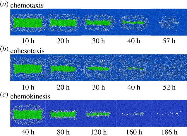
Snapshots of wound tissue under different guidance mechanisms of cell migration. (a–c) Snapshots of tissue during re-epithelialization under the three different guidance mechanisms. Blue: keratinocytes; green: wound elements and light blue: migrating keratinocytes.

Figure 7.

Re-epithelialization rate and cell migration speed under different guidance mechanisms. (a) Wound closure ratio r(t_N) over time under the three different guidance mechanisms. (b) Average migration speed s(t_N) of keratinocytes during re-epithelialization in regions at varying distances from the wound edge: Regions I: 0–80 μm, II: 80–160 μm, III: 160–240 μm, IV: greater than 240 μm. The error bars depict the standard deviations of three simulation runs.

We also measured the migration speed s(t_N), which is defined as the total length of the migrating trajectory over migrating time. Cells under cohesotaxis exhibited the highest migration speed in Region I, with s(t_N) = 3.4 ± 0.1 μm h⁻¹. By contrast, the migration speed under chemotaxis in Region I was only s(t_N) = 2.8 ± 0.1 μm h⁻¹. Under both chemotaxis and cohesotaxis, the migration speed in Region I is comparable with the physiological range of the observed speed of single keratinocyte migration of ∼5 μm h⁻¹ [41,42]. Under chemokinesis, however, the migration speed was only s(t_N) = 0.9 ± 0.1 μm h⁻¹, which was much slower than that of other mechanisms with guidance of a directional cue (figure 7b).

These results indicate that directional cues to guide cell migration are essential for wound tissue to achieve the rapid cell migration that is necessary for in-time re-epithelialization.

4. Discussion

In this study, we developed a novel computational model called DyCelFEM. It accounts for detailed changes in cellular shapes and mechanics of a large population of interacting cells. It can model the full range of cell motion, from free movement of individual cells to large scale collective cell migration. Furthermore, the transmission of mechanical forces via intercellular adhesion and its rupture is also modelled. In addition, our preliminary results suggest that an accurate account of cell morphology such as changes of cell–cell boundaries is important for timely re-epithelialization (data not shown). With the intracellular protein signalling networks embedded in individual cells, biochemical control of cell behaviours can also be modelled. Overall, the DyCelFEM model can be used to study biological processes involving 10³⁻⁴ of migrating cells subject to dynamic changes in shape and mechanics.

We applied the DyCelFEM method to examine the effects of biochemical and mechanical cues in regulating cell migration and in controlling tissue patterning during the re-epithelialization process using a simplified wound tissue model. Our results show that biochemical cues have local influence over the tissue (figure 6a), while mechanical cues have more global impact on the tissue. This is similar to observations from a previous study where the migrating cue taken from the intercellular force regulated by merlin protein showed long-distance influence on the cells [43]. In addition, biochemical cues are better at guiding cell migration with improved directionality and higher persistence (figure 4a,b), while mechanical cues are better at coordinating collective migration of cells (figure 4c). Based on comparison with in vitro studies [38,39], our results suggest that biochemical cues likely play dominant roles in guiding the migration of cells located in the regions surrounding wounds.

A previous study has also shown that small wounds can be closed without cell proliferation [44]. This can be simulated by setting α₁ in equation (2.10) to zero. Our results showed that under non-proliferative conditions, wound closure with both chemotaxis and cohesotaxis cues can be faster if the proportion of migrating cells increases. However, there are large lesioned and unsealed gaps remaining upon completion of re-epithelialization, as there are insufficient fresh cells to fill the wound bed. Overall, our results suggest that cell proliferation is essential for full closure of large wounds (see electronic supplementary material, text S8 for more details).

In this study, we examined the roles of mechanical and chemical cues separately. In reality, these two types of cue are coupled and entangled, and cooperatively regulate overall cell behaviour. For example, chemotactic cues can modulates integrins and influence adhesion of cells to the substrate [45]. Adhesion to the substrate can in turn influence signalling networks, which then alter cell–cell adhesion [32]. There are examples where mechanical cues can promote the directionality and persistence of cell migration, and biochemical signalling can influence cell mechanics and the collective behaviour of cells. For example, it was reported that mechanical cues from changes in collagen topography in the ECM can improve the persistence of cancer cell migration [46]. In addition, the merlin protein can serve as a mechanochemical transducer to help coordinate collective cell migration [43]. To understand such complex phenomena, more detailed networks of paracrine signalling and feedback loops between cells and their environmental matrix need to be developed and incorporated in our model. In summary, further improvement in the DyCelFEM model, additional in vivo and in silico studies are necessary to draw further conclusions on the roles of biochemical and mechanical cues in specific in vivo settings.

There are a number of limitations of our wound model. First, we did not consider the purse-string mechanism of wound healing. Cell crawling and acto-myosin cable contraction in a purse-string manner are the two well-known mechanisms driving epithelial wound closure [47]. While the former plays dominant roles in the closure of small defects (about 20 cells) [48], our study focus on closure of wounds of larger size where the mechanism of cell crawling driven by protrusion takes the dominant role [44]. Therefore, the purse-string mechanism is not considered in our current model (see more details in electronic supplementary material, text S5). Second, we did not consider realistic adhesion-coupling between cells. A possible improvement would be to model the adhesion between cells as springs with the adhesion force depending on the displacement of the two vertices of the adhesive contact. Currently, the scale of vertex displacement in our model is at the level of micrometres, which is much larger than the scale of cellular adhesion, which is usually at the level of nanometres [49]. Therefore, we simplify and treat cell–cell adhesion in our model using constant force. Third, our model is also limited as there is no feedback loops from cell–ECM interactions on cadherin-based cell–cell interactions and migration depends only on cell–cell adhesion. Although cells in counterproductive migration, where cells move away from the wound bed, are seen (figure 4a, intervals between 150° and 210°), neither large-scale movement nor extensive swirling are observed. However, these limitations can be removed with further development of DyCelFEM.

Authors' contributions

Conceived and designed the experiments: J.Z., Y.C., L.A.D. and J.L. Performed the experiments: J.Z. and Y.C. Analysed the data: J.Z., Y.C. and J.L. Wrote the paper: J.Z., Y.C., L.A.D. and J.L.

Competing interests

We declare we have no competing interests.

Funding

We would like to acknowledge NIH grant no. GM079804, GM50875 and NSF grant no. MCB-1415589 for financial support.

References

- 1.Alberts B, Johnson A, Lewis J, Morgan D, Raff M, Roberts K, Walter P. 2008. Molecular biology of the cell. New York, NY: Garland. [Google Scholar]
- 2.Weber GF, Bjerke MA, DeSimone DW. 2012. A mechanoresponsive cadherin–keratin complex directs polarized protrusive behavior and collective cell migration. Dev. Cell 22, 104–115. ( 10.1016/j.devcel.2011.10.013) [DOI] [PMC free article] [PubMed] [Google Scholar]
- 3.Brugués A. et al. 2014. Forces driving epithelial wound healing. Nat. Phys. 10, 683–690. ( 10.1038/nphys3040) [DOI] [PMC free article] [PubMed] [Google Scholar]
- 4.Oakes PW, Banerjee S, Marchetti CM, Gardel M. 2014. Geometry regulates traction stresses in adherent cells. Biophys. J. 107, 825–833. ( 10.1016/j.bpj.2014.06.045) [DOI] [PMC free article] [PubMed] [Google Scholar]
- 5.Arciero JC, Mi Q, Branca MF, Hackam DJ, Swigon D. 2011. Continuum model of collective cell migration in wound healing and colony expansion. Biophys. J. 100, 535–543. ( 10.1016/j.bpj.2010.11.083) [DOI] [PMC free article] [PubMed] [Google Scholar]
- 6.Lee P, Wolgemuth CW. 2011. Crawling cells can close wounds without purse strings or signaling. PLoS Comput. Biol. 7, e1002007 ( 10.1371/journal.pcbi.1002007) [DOI] [PMC free article] [PubMed] [Google Scholar]
- 7.Cochet-Escartin O, Ranft J, Silberzan P, Marcq P. 2014. Border forces and friction control epithelial closure dynamics. Biophys. J. 106, 65–73. ( 10.1016/j.bpj.2013.11.015) [DOI] [PMC free article] [PubMed] [Google Scholar]
- 8.Chen N, Glazier JA, Izaguirre JA, Alber MS. 2007. A parallel implementation of the cellular potts model for simulation of cell-based morphogenesis. Comput. Phys. Commun. 176, 670–681. ( 10.1016/j.cpc.2007.03.007) [DOI] [PMC free article] [PubMed] [Google Scholar]
- 9.Xu Z, Chen N, Kamocka M, Malgorzata M, Rosen E, Alber M. 2008. A multiscale model of thrombus development. J. R. Soc. Interface 5, 705–722. ( 10.1098/rsif.2007.1202) [DOI] [PMC free article] [PubMed] [Google Scholar]
- 10.Albert PJ, Schwarz US. 2016. Dynamics of cell ensembles on adhesive micropatterns: bridging the gap between single cell spreading and collective cell migration. PLoS Comput. Biol. 12, e1004863 ( 10.1371/journal.pcbi.1004863) [DOI] [PMC free article] [PubMed] [Google Scholar]
- 11.Nagai T, Honda H. 2009. Computer simulation of wound closure in epithelial tissues: cell–basal-lamina adhesion. Phys. Rev. E 80, 061903 ( 10.1103/physreve.80.061903) [DOI] [PubMed] [Google Scholar]
- 12.Vitorino P, Hammer M, Kim J, Meyer T. 2011. A steering model of endothelial sheet migration recapitulates monolayer integrity and directed collective migration. Mol. Cell. Biol. 31, 342–350. ( 10.1128/mcb.00800-10) [DOI] [PMC free article] [PubMed] [Google Scholar]
- 13.Basan M, Elgeti J, Hannezo E, Rappel WJ, Levine H. 2013. Alignment of cellular motility forces with tissue flow as a mechanism for efficient wound healing. Proc. Natl Acad. Sci. USA 110, 2452–2459. ( 10.1073/pnas.1219937110) [DOI] [PMC free article] [PubMed] [Google Scholar]
- 14.Newman T. 2005. Multicellular systems using subcellular elements. Math. Biosci. Eng. 2, 613–624. [DOI] [PubMed] [Google Scholar]
- 15.Rejniak KA. 2007. An immersed boundary framework for modelling the growth of individual cells: an application to the early tumour development. J. Theor. Biol. 247, 186–204. ( 10.1016/j.jtbi.2007.02.019) [DOI] [PubMed] [Google Scholar]
- 16.Hutson MS, Veldhuis J, Ma X, Lynch HE, Cranston PG, Wayne Brodland G. 2009. Combining laser microsurgery and finite element modeling to assess cell-level epithelial mechanics. Biophys. J. 97, 3075–3085. ( 10.1016/j.bpj.2009.09.034) [DOI] [PMC free article] [PubMed] [Google Scholar]
- 17.Vermolen F, Gefen A. 2015. Semi-stochastic cell-level computational modelling of cellular forces: application to contractures in burns and cyclic loading. Biomech. Model. Mechanobiol. 14, 1181–1195. ( 10.1007/s10237-015-0664-2) [DOI] [PubMed] [Google Scholar]
- 18.Osborne JM, Fletcher AG, Pitt-Francis JM, Maini PK, Gavaghan DJ. 2016. Comparing individual-based approaches to modelling the self-organization of multicellular tissues. bioRxiv, 074351 ( 10.1101/074351) [DOI] [PMC free article] [PubMed] [Google Scholar]
- 19.Kachalo S, Naveeed H, Cao Y, Zhao J, Liang J. 2015. Mechanical model of geometric cell and topological algorithm for cell dynamics from single-cell to formation of monolayered tissues with pattern. PLoS ONE 10, e0126484 ( 10.1371/journal.pone.0126484) [DOI] [PMC free article] [PubMed] [Google Scholar]
- 20.Li Y, Naveed H, Kachalo S, Xu LX, Liang J. 2014. Mechanisms of regulating tissue elongation in drosophila wing: Impact of oriented cell divisions, oriented mechanical forces, and reduced cell size. PLoS ONE 9, e086725 ( 10.1371/journal.pone.0086725) [DOI] [PMC free article] [PubMed] [Google Scholar]
- 21.Li Y, Naveed H, Kachalo S, Xu LX, Liang J. 2012. Mechanisms of Regulating Cell Topology in Proliferating Epithelia: Impact of Division Plane, Mechanical Forces, and Cell Memory. PLoS ONE 7, e43108 ( 10.1371/journal.pone.0043108) [DOI] [PMC free article] [PubMed] [Google Scholar]
- 22.Graner F, Glazier JA. 1992. Simulation of biological cell sorting using a two-dimensional extended potts model. Phys. Rev. Lett. 69, 2013 ( 10.1103/physrevlett.69.2013) [DOI] [PubMed] [Google Scholar]
- 23.Schiff LI. 1968. Quantum mechanics, 3rd edn New York, NY: M cGraw-Hill. [Google Scholar]
- 24.Tayllamin B, Mendez S, Moreno R, Chau M, Nicoud F. 2010. Comparison of body-fitted and immersed boundary methods for biomechanical applications. In Proc. of the Fifth European Conf. on Computational Fluid Dynamics, ECCOMAS CFD 2010, Lisbon, Portugal, 14–17 June (eds JCF Pereira, A Sequeira), pp. 1–20. [Google Scholar]
- 25.Brodland GW, Viens D, Veldhuis JH. 2007. A new cell-based FE model for the mechanics of embryonic epithelia. Comput. Methods Biomech. Biomed. Eng. 10, 121–128. ( 10.1080/10255840601124704) [DOI] [PubMed] [Google Scholar]
- 26.Larjava H, Häkkinen L, Koivisto L. 2011. Re-epithelialization of wounds. Endod. Top. 24, 59–93. ( 10.1111/etp.12007) [DOI] [Google Scholar]
- 27.Edelsbrunner H. 2001. Geometry and topology for mesh generation. Cambridge monographs on applied and computational mathematics Cambridge, UK: Cambridge University Press. [Google Scholar]
- 28.Bonakdar N, Gerum R, Kuhn M, Sporrer M, Lippert A, Schneider W, Aifantis K, Fabry B. 2016. Mechanical plasticity of cells. Nat. Mater. 15, 1090–1094. ( 10.1038/nmat4689) [DOI] [PubMed] [Google Scholar]
- 29.Dong S, Long Z, Tang L, Jiang Y, Yan Y. 2014. Simulation of growth and division of 3D cells based on finite element method. Int. J. Appl. Mech. 6, 1450041 ( 10.1142/S1758825114500410) [DOI] [Google Scholar]
- 30.Keren K, Pincus Z, Allen GM, Barnhart EL, Marriott G, Mogilner A, Theriot JA. 2008. Mechanism of shape determination in motile cells. Nature 453, 475–480. ( 10.1038/nature06952) [DOI] [PMC free article] [PubMed] [Google Scholar]
- 31.Zielinski R, Mihai C, Kniss D, Ghadiali SN. 2013. Finite element analysis of traction force microscopy: influence of cell mechanics, adhesion, and morphology. J. Biomech. Eng. 135, 071009 ( 10.1115/1.4024467) [DOI] [PMC free article] [PubMed] [Google Scholar]
- 32.Ng MR, Besser A, Danuser G, Brugge JS. 2012. Substrate stiffness regulates cadherin-dependent collective migration through myosin-II contractility. J. Cell Biol. 199, 545–563. ( 10.1083/jcb.201207148) [DOI] [PMC free article] [PubMed] [Google Scholar]
- 33.Menon SN, Flegg JA, McCue SW, Schugart RC, Dawson RA, Sean McElwain DL. 2012. Modelling the interaction of keratinocytes and fibroblasts during normal and abnormal wound healing processes. Proc. R. Soc. B. 279, 3329–3338. ( 10.1098/rspb.2012.0319) [DOI] [PMC free article] [PubMed] [Google Scholar]
- 34.Petrie RJ, Doyle AD, Yamada KM. 2009. Random versus directionally persistent cell migration. Nat. Rev. Mol. Cell Biol. 10, 538–549. ( 10.1038/nrm2729) [DOI] [PMC free article] [PubMed] [Google Scholar]
- 35.Roca-Cusachs P, Sunyer R, Trepat X. 2013. Mechanical guidance of cell migration: lessons from chemotaxis. Curr. Opin. Cell Biol. 25, 543–549. ( 10.1016/j.ceb.2013.04.010) [DOI] [PubMed] [Google Scholar]
- 36.Vedel S, Tay S, Johnston DM, Bruus H, Quake SR. 2013. Migration of cells in a social context. Proc. Natl Acad. Sci. USA 110, 129–134. ( 10.1073/pnas.1204291110) [DOI] [PMC free article] [PubMed] [Google Scholar]
- 37.Tremel A, Cai A, Tirtaatmadia N, Hughes BD, Stevens GW, Landman KA, O'Connor AJ. 2008. Cell migration and proliferation during monolayer formation and wound healing. Chem. Eng. Sci. 64, 247–253. ( 10.1016/j.ces.2008.10.008) [DOI] [Google Scholar]
- 38.Garlick JA. 2007. Engineering skin to study human disease–tissue models for cancer biology and wound repair. In Tissue engineering II, pp. 207–239. Berlin, Germany: Springer. [DOI] [PubMed] [Google Scholar]
- 39.Safferling K, Sütterlin T, Westphal K, Ernst C, Breuhahn K, James M, Jäger D, Halama N, Grabe N. 2013. Wound healing revised: a novel reepithelialization mechanism revealed by in vitro and in silico models. J. Cell Biol. 203, 691–709. ( 10.1083/jcb.201212020) [DOI] [PMC free article] [PubMed] [Google Scholar]
- 40.Epstein FH, Singer AJ, Clark RA. 1999. Cutaneous wound healing. N. Engl. J. Med. 341, 738–746. ( 10.1056/NEJM199909023411006) [DOI] [PubMed] [Google Scholar]
- 41.Kirfel G, Rigort A, Borm B, Schulte C, Herzog V. 2003. Structural and compositional analysis of the keratinocyte migration track. Cell Motil. Cytoskelet. 55, 1–13. ( 10.1002/cm.10106) [DOI] [PubMed] [Google Scholar]
- 42.Laplante AF, Germain L, Auger FA, Moulin V. 2015. Mechanisms of wound reepithelialization: hints from a tissue-engineered reconstructed skin to long-standing questions. FASEB J. 15, 2377–2389. ( 10.1096/fj.01-0250com) [DOI] [PubMed] [Google Scholar]
- 43.Das T, Safferling K, Rausch S, Grabe N, Boehm H, Spatz JP. 2015. A molecular mechanotransduction pathway regulates collective migration of epithelial cells. Nat. Cell Biol. 17, 276–287. ( 10.1038/ncb3115) [DOI] [PubMed] [Google Scholar]
- 44.Ravasio A. et al. 2015. Gap geometry dictates epithelial closure efficiency. Nat. Commun. 6, 7683 ( 10.1038/ncomms8683) [DOI] [PMC free article] [PubMed] [Google Scholar]
- 45.Weber G, Bjerke MA, DeSimone DW. 2011. Integrins and cadherins join forces to form adhesive networks. J. Cell Sci. 124, 1183–1193. ( 10.1242/jcs.064618) [DOI] [PMC free article] [PubMed] [Google Scholar]
- 46.Riching K. et al. 2014. 3D collagen alignment limits protrusions to enhance breast cancer cell persistence. Biophys. J. 107, 2546–2558. ( 10.1016/j.bpj.2014.10.035) [DOI] [PMC free article] [PubMed] [Google Scholar]
- 47.Begnaud S, Chen T, Delacour D, Mege RM, Ladoux B. 2016. Mechanics of epithelial tissues during gap closure. Curr. Opin. Cell Biol. 42, 52–62. ( 10.1016/j.ceb.2016.04.006) [DOI] [PMC free article] [PubMed] [Google Scholar]
- 48.Vedula SRK. et al. 2015. Mechanics of epithelial closure over non-adherent environments. Nat. Commun. 6, 6111 ( 10.1038/ncomms7111) [DOI] [PMC free article] [PubMed] [Google Scholar]
- 49.Hynes R. 1992. Integrins: versatility, modulation, and signaling in cell adhesion. Cell 69, 11–25. ( 10.1016/0092-8674(92)90115-S) [DOI] [PubMed] [Google Scholar]
Associated Data
This section collects any data citations, data availability statements, or supplementary materials included in this article.