GW-SEM: A Statistical Package to Conduct Genome-Wide Structural Equation Modeling

Abstract

Improving the accuracy of phenotyping through the use of advanced psychometric tools will increase the power to find significant associations with genetic variants and expand the range of possible hypotheses that can be tested on a genome-wide scale. Multivariate methods, such as Structural Equation Modeling (SEM), are valuable in the phenotypic analysis of psychiatric and substance use phenotypes, but these methods have not been integrated into standard genome-wide association analyses because fitting a SEM at each single nucleotide polymorphism (SNP) along the genome was hitherto considered to be too computationally demanding. By developing a method that can efficiently fit SEMs, it is possible to expand the set of models that can be tested. This is particularly necessary in psychiatric and behavioral genetics, where the statistical methods are often handicapped by phenotypes with a large components of stochastic variance. Due to the enormous amount of data that genome-wide scans produce, the statistical methods used to analyze the data are relatively elementary and do not directly correspond with the rich theoretical development, and lack the potential to test more complex hypotheses about the measurement of, and interaction between, comorbid traits. In this paper, we present a method to test the association of a SNP with multiple phenotypes or a latent construct on a genome-wide basis using a Diagonally Weighted Least Squares (DWLS) estimator for four common SEMs: a one-factor model, a one-factor residuals model, a two-factor model, and a latent growth model. We demonstrate that the DWLS parameters and p-values strongly correspond with the more traditional Full Information Maximum Likelihood parameters and p-values. We also present the timing of simulations and power analyses and a comparison with and existing multivariate GWAS software package.

Introduction

With the proliferation of genome wide association data and the development of high-speed, low-cost whole genome and exome sequencing, the availability of high quality genomic data has rapidly and greatly increased (Paltoo et al., 2014). The initial benefit of genome wide association studies (GWAS) was seen in the areas of common physical diseases such as heart disease, auto-immune disorders and diabetes (Visscher, Brown, McCarthy, & Yang, 2012). These disorders have largely unambiguous symptoms that make them relatively easy to measure with high levels of precision. More recently, there have been genetic associations for psychiatric disorders, such as schizophrenia (Schizophrenia Psychiatric Genome-Wide Association Study (GWAS) Consortium, 2011) or cigarette smoking (Lips et al., 2010; Liu et al., 2010; Saccone et al., 2009), major depressive disorder (CONVERGE consortium, 2015; Hyde et al., 2016), neuroticism (Okbay et al., 2016; Smith et al., 2016), and bipolar disorder (Muhleisen et al., 2014). Early GWASs of psychiatric phenotypes were based on the assumption that there existed single variants with large effect sizes that influenced complex traits. Years of collaboration that amassed very large datasets have subsequently shown that assumption to be false: most complex phenotypes are highly polygenic. Hundreds, if not thousands, of genetic variants with very small effect sizes contribute to variation in complex, multidimensional, imprecisely measured phenotypes. Today, very large sample sizes continue to be needed to compensate for the low statistical power to detect genetic associations for these complex traits. Increasing the precision by which phenotypes are measured, using the Structural Equation Modeling (SEM) techniques proposed herein, should enhance our ability to find significant associations and will expand the possible hypotheses that can be tested on a genome wide basis.

While some multivariate GWAS (MV-GWAS) methods allow for the association of a SNP with multiple phenotypes, they do not closely correspond with the analytical techniques used in multivariate or developmental analyses of the respective phenotypes. This disconnect limits the extent to which identified genetic associations can improve our understanding of the etiology and progression of a disorder. For example, current MV-GWAS methods rely on various statistical techniques such as multivariate regression (multiple DV’s), canonical correlation analysis and MANOVA (MV-PLINK – Ferreira & Purcell, 2009), simultaneously regressing the SNP on multiple phenotypes (MultiPhen – OReilly et al., 2012), imputation based methods (MV-SNPTEST – Marchini, Howie, Myers, McVean, & Donnelly, 2007, MV-BIMBAM – Stephens, 2013; Servin & Stephens, 2007, and PHENIX – Dahl et al., 2016), principal components analysis (PCHAT – Klei, Luca, Devlin, & Roeder, 2008), multivariate linear mixed modeling (GEMMA – Zhou & Stephens, 2014, 2012; mvLMM – Furlotte & Eskin, 2015; Wombat – Meyer & Tier, 2012), or meta-analytic procedures (TATES – van der Sluis, Posthuma, & Dolan, 2013). SEM methods have been applied genome-wide with twin and family models using FIML estimators (Medland & Neale, 2010; Medland et al., 2009; Fardo, 2014; Kent et al., 2009; Choh et al, 2014) in Classic MX (Neale, 1994) or SOLAR (Blangero et al., 2000), which is particularly relevant because twin and family models utilize SEM techniques and each family members has a unique phenotype and as such could be considered multivariate SEM GWAS. While these diverse MV-GWAS methods estimate the relationship between a SNP and multiple phenotypes, to increase the efficiency of optimization it is necessary to restrict the potential flexibility of each method, and therefore the variety of hypotheses that can be tested. Moreover, these methods may be unfamiliar to substantive researchers who lack broad training in statistics and genomics. As such, they may not be germane to commonly encountered scenarios in psychiatric genetics. Nevertheless, these existing multivariate GWAS techniques typically yield greater statistical power than univariate methods that rely on sum- or factor-score approaches, and this benefit can be retained in GW-SEM.

Because these MV-GWAS methods do not necessarily dovetail with the phenotypic (non-genetic) methods, many researchers summarize multivariate data into sum- or factor-scores that can be analyzed with existing univariate GWAS methods (Purcell et al., 2007; Laird, 2011; Abecasis, Cherny, Cookson, & Cardon, 2002). While this univariate approach is very rapid and may approximate a MV-GWAS under some circumstances, a trait or disorder may be better modeled as a latent factor that would be only approximated by a sum-score or a diagnosis. Further, factor score indeterminacy may produce erroneous scores, or bias the standard errors of the parameters thereby inflating the test statistics and Type I Error rates (Grice, 2001). More importantly, constructing these scores negates any possibility for testing alternative, and truly multivariate, hypotheses that may inform our understanding of the phenotype. While preliminary methods for exploring the effects of SNPs on phenotypes can provide important insights into genetic associations, the statistical tools necessary to deliver additional insights can be improved.

Finally, existing GWAS methods typically treat ordinal variables as either continuous or binary. Treating ordinal items as continuous can result in biased parameters estimates and incorrect standard errors and model test statistics (Muthen, 1984; Agresti, 2002; Johnson & Creech, 1983). Alternatively, treating ordinal items as binary reduces the power to detect significant associations. Therefore, treating ordinal items appropriately will reduce the bias in the parameter estimates while maximizing power.

GW-SEM utilizes Structural Equation Modeling (SEM), a common method in psychology and psychiatry. The approach closely corresponds to the conceptualization of phenotypes derived from DSM-V diagnoses of psychiatric and substance use disorders. This interpretation of a diagnosis implies that one’s liability on a latent trait can be indexed by a number of specific symptoms or behaviors (e.g., nicotine dependence leads individuals to smoke more cigarettes per day, have a harder time abstaining in socially inappropriate circumstances, and to experience more intense cravings for nicotine). This idea, known more broadly as the common factor model, depicted in in Fig. 1a, is the natural extension of the current GWAS methods for multiple phenotypes. The common factor model is a special case of a larger set of Structural Equation Models (SEMs) that are routinely applied to phenotypes in the psychiatric genetics literature. For example, multiple factor models are routinely used to examine comorbidity between phenotypes (Doyle, Murphy, & Shevlin, 2016; Carragher et al., 2016; Krueger, 1999), and Latent Growth Models (LGMs) are widely used to examine developmental trajectories (S. C. Duncan, Duncan, & Strycker, 2006; T. E. Duncan et al., 1997; Neale & McArdle, 2000).

Figure 1. Schematic Representations of the Structural Equation Models that can be fit using the GW-SEM package.

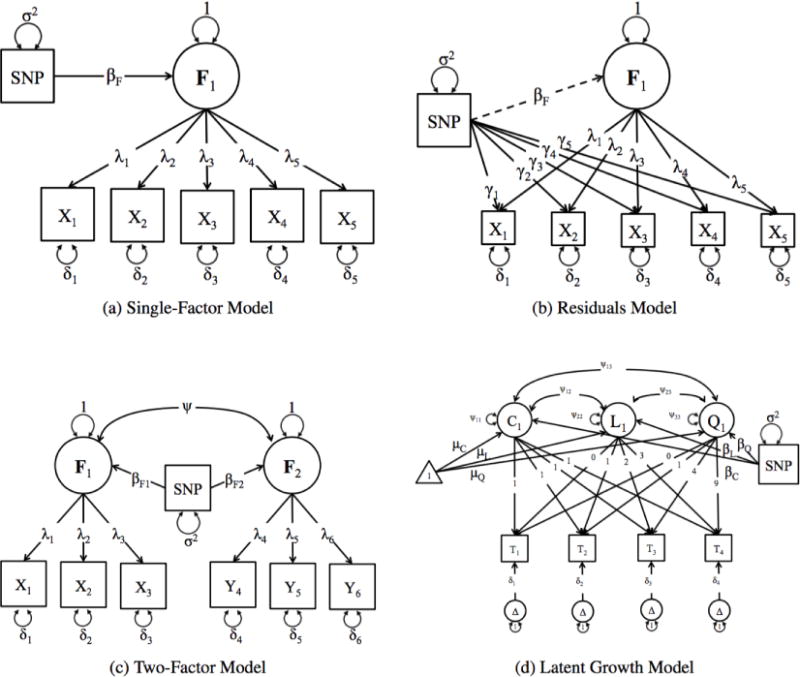
Fig. 1a presents the one-factor model, in which a latent factor (F₁) causes the observed items (x_k). The association between the latent factor and the observed indicators are estimated by the factor loadings (λ_k). The residual variances (δ_k) indicate the variance in x_k that is not shared with the latent factor. The regression of the latent factor on the SNP (for all SNPs in the analysis) is depicted by β_F. Fig. 1b presents the residuals model, which has very similar parameters to the one-factor model, with the notable difference that the individual items are regressed on each SNP (γ_k). Fig. 1c presents the two-factor model. In this model, both latent factors (F₁ & F₂) are regressed on every SNP (β_F1 & β_F2) and the latent factors are allowed to correlate (ψ). Finally, Fig. 1d presents the latent growth model, where the factor loadings are fixed to specified values, and the means (μ_F), variances and covariances (Ψ) of the latent growth parameters are estimated. Each latent growth factor is then regressed on each SNP (β_F).

Furthermore, comorbidity within and between psychiatric and substance use disorders is often substantial (Kessler, Chiu, Demler, & Walters, 2005; Cross-Disorder Group of the Psychiatric Genomics Consortium, 2013), implying that the genetic factors associated with one phenotype (e.g. smoking) may be shared with other logically distinct but correlated phenotypes (e.g. schizophrenia). These pleiotropic expectations must take the correlation between the phenotypes into consideration in order to accurately estimate the association between a SNP and either phenotype. This type of pleiotropy (two latent factors regressed on a single SNP) cannot be directly specified in current GWA methods. To test such hypotheses requires a GWAS method that directly uses SEM.

There are several reasons why SEM methods are not commonly used in a genome-wide context. First, GWAS utilze an immense amount of data for each subject. While this may seem beneficial, from a data analysis perspective colossal datasets pose massive challenges for analysis. Consequently, any statistical procedure that is employed must be either hypothesis driven, such as candidate gene studies, or extremely fast so as to process millions of analyses in a reasonable amount of time. Methods that are computationally intensive are not feasible when millions of tests are conducted. This limitation is only going to become more difficult to deal with as GWAS data becomes more available through data sharing agreements such as The Database of Genotypes and Phenotypes (DbGaP).

Second, each additional parameter that is added to a statistical model exponentially increases the computational complexity. Thus, univariate models are computationally efficient, but as the model gets more complex (by increasing the number of variables) computation time increases. This is especially true when numerical optimization is required to estimate model parameters. While certain statistical shortcuts can make it relatively easy to calculate associations, many do not generalize to the multivariate case.

Specifically, many CFA models rely on Maximum Likelihood (ML) Estimators that are computationally intensive. While ML estimators have excellent statistical properties (they are asymptotically unbiased and have minimum variance of asymptotically unbiased estimators), converging to ML solutions via numerical optimization can be computationally demanding. This is especially true for ordinal indicators that are so pervasive in psychiatric, substance use and psychological assessments. There have been several attempts to estimate genetic associations with latent factors within an SEM context using ML (Medland and Neale, 2010; Medland et al., 2009, Fardo et al., 2014; Kent et al., 2009; Choh et al, 2014). ML algorithms, however, are computationally intensive (taking 30 seconds per SNP) and may be prone to optimization failures. These limitations make conducting SEM analyses on a genome wide scale impractical for many researchers.

Finally, as alluded to above, most phenotypes, especially those in psychology and psychiatry, have binary (Yes or No) or ordinal (None, A Little, Some, A Lot) response options, which greatly increases the numerical complexity of optimization. Under the normal threshold model, the likelihood must be calculated using numerical integration of the multivariate normal distribution (or by repeated integration of the conditional normal distribution while integrating over the factors; Bock & Aitkin, 1981). The complexity increases exponentially with either the number of items or the number of factors. This difficulty in part led to the development of asymptotic weighted least squares estimators by Browne and others (Browne, 1984; Joreskog & Sorbom, 1993).

While the challenges noted above are serious, several solutions exist that can attenuate the most difficult ones. While the ‘Big Data’ problem will get worse as genotyping becomes cheaper, the solution to this problem is partially solved by relying on alternative estimators. One alternative is to rely on Least Squares (LS) estimation procedures (especially diagonally weighted least squares, DWLS), which greatly reduce the computational complexity. Given sufficiently rapid methods, it becomes possible to fit a SEM millions of times, one for each measured SNP. Furthermore, while adding parameters to a model increases processing time with any estimation procedure, it does not necessarily become prohibitive if the model converges rapidly.

Model Fitting and Optimization

In this section we discuss the details of the estimation process, along with the algebra for calculating the weights and the estimation of the SEM. All of the code is written for the R computing environment (R Development Core Team, 2008) and OpenMx (Neale et al., in press; S. M. Boker et al., 2015; S. Boker et al., 2011) is used to fit the models.

Briefly, a 4-step procedure is followed. In the first, the SNP invariant covariances and weights are computed. Second, the covariances between the items/covariates and each SNP and the associated weights are calculated. Third, the individual SNP covariances are appended to the SNP invariant covariance matrix. Finally, the specific model from Fig. 1 is fit to the covariance matrix using a DWLS estimation procedure. GW-SEM requires the user to provide a phenotype and genotype file, with individuals on the rows and items or SNPs on the columns, respectively. The genotype data must be properly QC’d prior to analysis. Then, by selecting one of the models from Fig. 1, the model is fit to the data. GW-SEM therefore provides a rapid, accurate and user-friendly method that can be applied to SEM with continuous, binary and ordinal items, along with genome-wide data. The data for GW-SEM may be either hard-called or dosage format data, however they will need to be formatted so that SNPs are on the columns and individuals are on the rows (See the tutorial for more details).

The first step in the GW-SEM algorithm is to calculate the SNP-invariant variance-covariance matrix and the associated weights. These are the variances and covariances of the indicators of the latent factor(s) and any covariates (such as age, sex or population stratification principal components), and the corresponding weights. Because these statistics are included in the SEM for every SNP, it is possible to calculate them once and re-use them in the analysis of every SNP. Different data types (continuous, ordinal and binary) may be used in an analysis, so SNP-invariant matrices are constructed from pairwise maximum-likelihood covariances between the variables. The function is designed to automatically detect the data type, and estimate the appropriate covariance for any pair of variables. These are covariances for pairs of continuous variables, tetrachoric/polychoric correlations for pairs of ordinal variables, and point-biserial covariances for mixed continuous-binary pairs of variables. Standard errors of the MLE’s are calculated during the same process. Finally, the weight matrix is constructed as follows:

$$W=\frac{\sqrt{N_j-1}}{{\mathit{SE}}_j}$$ (1)

where N_j is the number of observations contributing to the j^th covariance, and SE_j is the standard error of the j^th covariance. Covariances with larger samples and/or smaller standard errors will have larger weights. This accounts for missing data patterns by using pairwise estimates of each variance, covariance, mean and threshold. As with most statistical procedures, data that are not missing at random may result in biased estimates. Thus, in contrast to other packages that use list-wise deletion (removing an entire observation if there is any missing value), the current package uses all of the available information, and is appropriate when the data are missing at random (Little & Rubin, 1989). This is particularly important for multivariate models, because an individual’s probability of missing a single variable increases with the number of variables per person. Further, for longitudinal models, this pair-wise procedure can greatly reduce the impact of attrition across time.

The next step is to estimate the SNP-item and SNP-covariate covariances. The covariances between the SNPs and both the items and the covariates must be estimated for each SNP. This step effectively conducts a univariate GWAS for each item and covariate; it is the longest and most computationally intensive part of the algorithm. To minimize the number of objects stored in the R environment, and therefore increase processing speed, this function accesses data that are not loaded into the R environment, but instead stored as *.txt files. As the raw files have the potential to be extremely large (even if the genotype data is separated into multiple files), all of the data management is done using unix functions. Subsets of SNPs are copied to much smaller temporary files and these temporary files are loaded into R. The covariance of each SNP with each item and covariate is then calculated, as is the mean and variance of the SNP. The number of analyses that are conducted are extremely large, storing the results in R would also hinder processing speed, so the estimated SNP-item and SNP-covariate covariances, weights and standard errors are written to external files. The covariances, standard errors and weights are calculated the same way as was done in step 1.

The final steps of the model is when the SEM is actually fit to the data. The DWLS fit function is:

$$\mathit{DWLS}=\frac{1}{2}\mathrm{tr}\left[{\left({\sum }_{\mathit{Obs}}-{\sum }_{\theta }\right)}^{2}W\right]$$ (2)

where Σ_θ is the expected covariance matrix, Σ_Obs is the observed covariance matrix, W is matrix of weights.

The expected covariance matrix, Σ_θ, is calculated using the standard Reticular Action Model (RAM: McArdle & McDonald, 1984; McArdle & Boker, 1990), which produces the same expectations as the LISREL model (Joreskog & Sorbom, 1989, 2001; Joreskog & Sorbom, 1996; Joreskog & Sorbom, 1996). The two approaches differ with respect to the size and number of the matrices involved in the calculation; the RAM model has 4 larger matrices, while the LISREL model has up to 13 smaller matrices. The algebra for the RAM expected covariance matrix is:

$${\sum }_{\theta }=F(I-A)S{(I-A)}^T{F}^T$$ (3)

where F is a filter matrix k (the number of observed variables) × m (the number of observed + latent variables), I is an m × m identity matrix, A is an m × m matrix with the Asymmetric (single-headed) paths, and S is an m × m matrix with the Symmetric (double-headed) paths. Accordingly, the residual variances and variances of exogenous variables are in the S matrix, while the factor loadings and regression paths are in the A matrix. Because the scripts are publicly available, the simplicity of the RAM matrices makes it possible for advanced users to edit the code and construct alternative SEM functions that are not included in the current software.

The observed covariance matrix is constructed using the SNP-invariant covariances obtained in step 1, and the SNP-item and SNP-covariate covariances obtained in step 2. For each SNP, the observed SNP-item and SNP-covariate covariances and the SNP variance are appended to the SNP-invariant covariance matrix, thereby providing a complete observed variance-covariance matrix. The weight matrix is constructed similarly.

While there is some debate about the reliability of LS estimators, previous research has demonstrated that DWLS and ML parameters are equally accurate when the data is continuous and multivariate normal, but that DWLS estimators may be slightly more accurate with categorical or non-normal data (Mindrila, 2010; Li, 2015). We directly address these questions below. For the current algorithm, the important difference between DWLS and FIML estimators is speed of optimization.

The expected relationships between the Items and Covariates

The observed covariances between the items and the covariates are estimated in the same way as covariances among the items, but the relationships between the items and the covariates in the expected covariance matrix are modeled in a very specific way, as there are multiple possible associations between the items and covariates. For the current models, the items are directly regressed on the covariates. This is in contrast to the alternative method where the latent variables were regressed on the covariates. While there are clear benefits to both strategies, the chosen method is slightly more conservative in that it uses additional parameters to capture these associations. Specifically, for each covariate, j, the model estimates k (the number of items) regression parameters, resulting in j × k estimates. In the alternative specification, one regression parameter is estimated for each covariate, resulting in j regression parameters. The alternative specification, however, imposes the assumption that the covariates are associated with the items proportional to their factor loadings, an assumption that is avoided in the current specification.

Essential Features of GW-SEM

GW-SEM is a method to fit a SEM on a genome-wide basis. The new software provides algorithms to fit 4 SEMs, presented in Fig. 1. Because the code is entirely open source, users to can modify and extend the methods to other types of SEM and for other types of data (e.g. fMRI data).

Comparison between DWLS and FIML

The diagonally weighted least squares estimator may not have the same desirable properties as full information maximum likelihood (FIML) estimators, making it necessary to compare the estimators via simulation. Although DWLS estimators appear to be asymptotically unbiased (DiStefano & Morgan, 2014), it is necessary to demonstrate unbiasedness for the current estimator. In doing so, it is possible to compare the efficiency and convergence of the DWLS and FIML estimators.

To compare the DWLS and the FIML methods, data were simulated for a one-factor model with four ordinal indicators and one covariate for 10,000 observations, along with 10,000 independent SNPs generated under the null hypothesis of no association. The factor loadings of the items on the latent factor, λ, were specified to be .7, .6, .5, and .4, with residual variance of each item being, δ = 1 − λ², so that the variance of each item was constrained to unity. The factor variance, ψ, was fixed at 1. Observed items were generated using the mvrnorm package in R (Venables & Ripley, 2002), which produces multivariate normal, continuous variables. To construct the ordinal items, the continuous data were split into four equally frequent ordinal categories. The SNPs were simulated from independent binomial distributions with minor allele frequencies ranging from .01 to .5. The simulated data were then analyzed with both the DWLS and the FIML fit functions for raw ordinal data. The key statistics for the purposes of GW-SEM are: i) the estimated regression parameters, ii) the p-values associated with these estimates, and iii) failures of model convergence. Any models that failed to converge were excluded from comparisons of the regression parameters and p-values.

The correlation between the regression parameters for the DWLS and FIML algorithms is very strong (r = .99), and the p-values for the DWLS and FIML algorithms is also very large (r = .96). Notably, there appears to be a small, though detectable, nonlinearity in the relationship between the p-values at the low end of the spectrum. This non-linearity appears to be a function of the minor allele frequency and variance of the SNPs. To further examine this relationship, Spearman’s rank-order correlations were calculated for the FIML p-values lower than .1, resulting in a correlation of r_spearman = .647. As most researchers are interested in the extreme tails of the p-value distribution, we also correlated the −log₁₀(p), which was also very large (r = .95). It is important to reiterate that the associations were simulated under the null model, making the extreme tails of the distribution quite rare, and contributing to the attenuation of the correlations. In toto, these results suggest that the estimates and and p-values from the DWLS procedure are extremely similar to those obtained by FIML.

To evaluate the Type I Error rate of the DWLS method in more detail, we examine the proportions of p-values that exceeded four critical thresholds: .10, .05, .01, and .001. The raw p-values from the DWLS procedure tend to be liberal with .1230 of the p-values falling below p = .1, .0669 falling below p = .05, .0159 falling below p = .01, and .0026 falling below p = .001. This implies inflation of the test statistic, t. To quantify this inflation, we calculated an inflation factor, $\sqrt{\frac{1}{n}{\displaystyle \sum t^2}}$, which should be theoretically equal to 1 but was 1.076 in the simulated sample. We then adjusted each test statistic by the inflation factor and recalculated the p-values. The resulting p-values followed the null distribution very closely: .0980 of the p-values were below p = .1; .0504 below p = .05; .0103 below p = .01, and .0012 below p = .001. Thus, while there may be a slight inflation of the raw DWLS p-values, the corrected DWLS p-values follow a null distribution, and the rank-order of p-values are consistent with the FIML statistics. Accordingly, we recommend that the DWLS algorithm be used as an initial screen for significant SNPs, and that the most promising ones be investigated further with the FIML algorithm to obtain more precise p-values.

Finally, it is possible to compare the likelihood of convergence problems for the DWLS and FIML estimators. Of the 10,000 SNPs that were analyzed, the DWLS estimator failed on 80 SNPs (.8% of the trials) while the FIML estimator failed on 793 SNPs (7.9% of the trials). Thus, convergence issues were much more frequent for the FIML estimator. SEM methods often struggle to converge when there are relatively large differences in the magnitude of the variance for the variables in the model. To further explore the DWLS convergence failures in more detail we examined the MAF for the convergence failures as SNPs with small MAFs have correspondingly small variances. For the 80 DWLS models that did not converge, the SNPs had minor allele frequencies ranging from .009 to .016 MAF. To put this in context, 218 SNPs had a MAF less than .02, meaning that approximately 1/3 of SNPs with a MAF less than .02 failed to converge using the DWLS algorithm. While DWLS convergence failures do not disrupt the estimation process, this implies that researchers should restrict their analyses to SNPs with MAFs larger than .02 with sample sizes in the 10,000 observation range. With smaller sample sizes (N < 5,000) MAFs larger than .05 may be prudent.

Timing

Next we addressed two key questions about timing via simulation: sample size and number of observed variables. Because sample size is unrelated to the time it takes to fit the SEM, the current timing studies focus on the SNP-Item and SNP-covariate correlations, the prerequisite steps for the SEM analyses.

To examine the time to estimate the covariances, a five-indicator model with three covariates for was fitted to datasets with 2,500, 5,000, or 10,000 observations. For all models, the factor loadings were simulated at .8, .7, .6, .5, and .4, with the residual variance of each item being, δ = 1 − λ². Again, the factor variance, ψ, was fixed at 1, and continuous, multivariate normal variables were simulated. The continuous data were used for the continuous models. For the ordinal models, the continuous data were split into four equally frequent categories, and a median split was used to create the binary data. The three covariates were simulated as independent random normal variables, to mimic the inclusion of ancestry principal components in the analysis. Each item was regressed directly on each covariate. The SNPs were again simulated from independent binomial distributions with minor allele frequencies ranging from .01 to .5. To examine the impact of adding items to the model, the same simulation process was employed, but only 3, 4 or 5 of the items were included in the analysis. For each timing study, 50,000 SNPs were simulated and were accessed in 1,000 SNP batches, providing 50 observed times for each timing condition. The mean and standard deviation of the time in minutes were then calculated. All simulations were conducted on dual 4-core or dual 6-core Intel Xeon 3.6GHz processors and 128–256 Gb RAM.

The first timing study addressed the impact of increasing sample size for 2,500, 5,000, and 10,000 observations with three different variable types : binary, ordinal, and continuous items and 3 continuous covariates. The results of the simulation are presented in Fig. 2a.

Figure 2. The average duration (in minutes) to estimate covariances between the SNPs, items, and covariates (error bars represent ± 1.96 standard deviations).

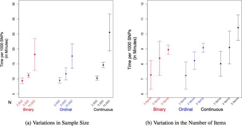
Fig. 2a presents the mean number of minutes (and standard deviations) to estimate covariances between 1,000 SNPs and 5 items and 3 covariates for 2,500, 5,000 and 10,000 observations for the one-factor model. Fig. 2b presents the mean number of minutes (and standard deviations) to estimate covariances between 1,000 SNPs and 3 covariates and 3, 4 and 5, items for 2,500 observations for the one-factor model.

As can be seen the Figure 2a, as sample sizes double from 2,500 to 5,000 to 10,000 observations, there is an exponential increase in the time it takes to estimate the covariances between SNP and the items and covariates for all item types. It is important to note, however, that for the smaller sample sizes there are no substantial differences in the time taken to estimate the categorical and the continuous correlations. When the sample size increases to 5,000 or 10,000, the continuous correlations take significantly longer. Specifically, for the ordinal data models, when the sample size is approximately 2,500, the algorithm takes 9.53 minutes to estimate the 8 necessary correlations for 1,000 SNPs (0.57 seconds per SNP), while when the sample size is 10,000 it takes 17.63 minutes to estimate the same number of correlations (1.06 seconds per SNP). As a point of comparison, using FIML it took 2 hours and 19 minutes to fit the same ordinal model to N=10,000 observations for a single SNP.

The second timing study assessed the impact of increasing the number of measures in the analysis. To examine this, three separate models were estimated with 3, 4 and 5 items (again with binary, ordinal and continuous items), and 3 continuous covariates with a sample size of 2,500. The results are presented in Fig. 2b. As can be seen in Figure 2, the increase in the time required to estimate correlations between an increasing numbers of items is approximately linear for all variable types. It is important to note that as the average computation time increases, the standard deviation of the mean convergence time also increases. This increase is in part due to traffic on the server that was not part of the timing study, but mimics realistic server conditions in many laboratories.

The final factor that affects processing time is the size of the genotype file. Large SNP files take longer to process. While it is possible for genotype files to be larger than 1 Tb, such files are very difficult to manage. To deal with these massive genotype files, most analysts create multiple genotype files. For example, 50,000 SNPs for 10,000 observations is approximately 1 Gb, which is still quite large, but computationally feasible. Individual users must balance file size and file proliferation concerns.

If we assume that it takes approximately 20 minutes to estimate associations for 1,000 SNPs, and the 1,000 Genomes Project reference imputation of well genotyped samples with R² ≥ .6 and MAF ≥ .05 covers approximately 6.5 million variants, it would take approximately 2267 hours of processing time to complete the analysis on a single thread of a cpu core. Capitalizing on the potential for parallel processing would reduce the processing time by a factor of the number of available processors. Thus, a standard laptop (with 2 dual-core multithreaded processors) would be able to process a 5-indicator CFA model for 6,500,000 SNPs in approximately 271 hours (11 days). On a server with parallel processing capacity, analysis time could be substantially reduced to a few hours. While this length of time is reasonable, it is inevitably slower than other MV-GWAS methods that treat the items as continuous variables (Zhou & Stephens, 2014, 2012; Furlotte & Eskin, 2015; Meyer & Tier, 2012).

Power

To calculate the power to detect a significant association, two models were fit using FIML: one freely estimating the effect of the SNP on the latent factor and one where the effect was fixed at zero. The difference in the −2 log-likelihoods of the two models follows a χ² distribution with one degree of freedom under the alternative hypothesis H_A. Importantly, the χ² value increases linearly with sample size, making it possible to extrapolate the expected χ² value across a range of sample sizes. This value can be used as the non-centrality parameter (NCP) for power calculation. Accordingly, the power to detect a genome-wide significant association for a 1 df test is $1-p\left({\chi }_{\mathrm{crit}}^2\right)$ where ${\chi }_{\mathrm{crit}}^2~{\chi }_1^2(\mathrm{ncp})$. In R, this can be done using the function: power = 1-pchisq(qchisq(1-5e-8, 1), 1, ncp), where 5e⁻⁸ is the value for genome wide significance for 1 df and ncp is the calculated non-centrality parameter for each sample size (see Verhulst, in press, for more details).

For the power analyses, a five-indicator model was simulated with all of the factor loadings fixed at .7, the residuals fixed at 1 − .7² = .51, and the factor variance fixed at 1. An association between the SNP and the latent factor was simulated to have an effect of .20, .10 or .05. To construct the SNP for each analysis, two minor allele frequencies were used: .25 and .05. As genetic theory provides excellent justifications of the mean and variance of a SNP (μ = 2p & σ² = 2p(1 − p), where p is the minor allele frequency), the SNP mean and variance was specified accordingly. All of the data was simulated using mvrnorm (Venables & Ripley, 2002), producing multivariate normal data. As done previously, the ordinal items were split into 4 equally sized ordinal categories. The SNP was split into three genotypes in such a way that the proportions of each genotype was in Hardy-Weinberg Equilibrium for the specified minor allele frequency. As transforming continuous variables into ordinal items and SNPs slightly changes the observed covariances, models were scrutinized to ensure that the estimated SNP regression parameters were within .001 of the simulated values for both the continuous and ordinal models.

We then examined the power to detect significant associations between a SNP and a single latent factor. The power to detect significant associations between a SNP and a latent variable from any of the models follows directly from existing SEM power analysis (Lai, 2011; MacCallum & Hong, 1997; Wolf, Harrington, Clark, & Miller, 2013; Miles, 2003; Chin, 1998). Two factors adversely affect statistical power to detect the trait-relevant genetic associations in many human traits of interest. One is that the variants typically have small effect sizes (of the order of 1% of variance or less). The second is that ordinal data are generally less precise than continuous measures. Therefore we present statistical power curves for several illustrative cases. Power curves for continuous and ordinal models, with minor allele frequencies (MAF) of .25 (relatively common allele) and .05 (relatively rare), and a range of effect sizes (β = .20, .10, & .05) are presented in Fig 3. These effect sizes would equate to a $\frac{1}{5}\mathit{sd}$ change between either homozygote and the heterozygote, a $\frac{1}{5}\mathit{sd}$ change between the minor allele homozygote and the major allele homozygote, or a $\frac{1}{10}\mathit{sd}$ change between the minor allele homozygote and the major allele homozygote.

Figure 3. Power to detect a genome-wide significant association with varying effect sizes and minor allele frequencies.

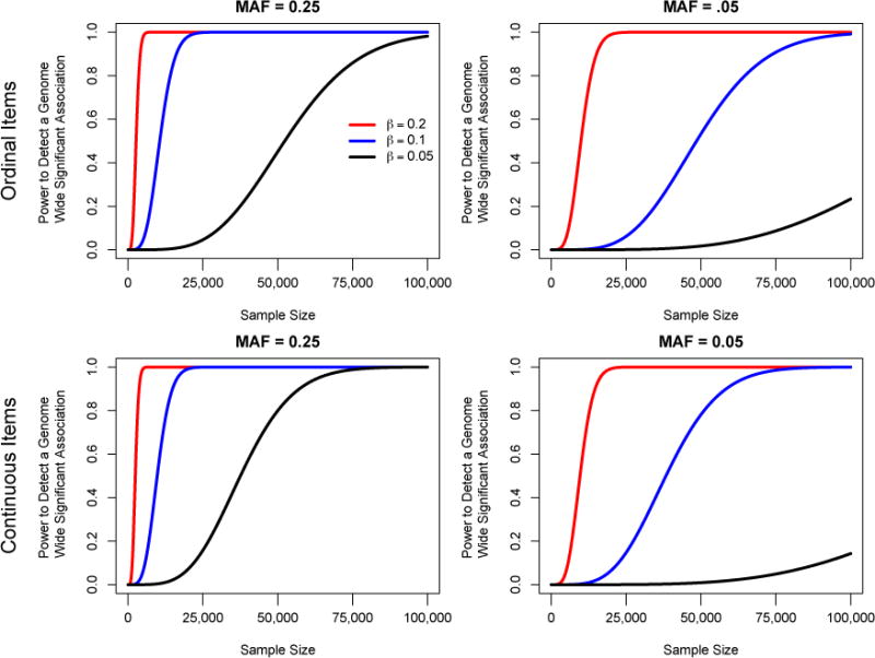
Fig. 3a–d present the power curves for the ability to detect genome-wide significant associations between a SNP and a latent factor for a one-factor model with 5 items for continuous and ordinal items and SNPs with a minor allele frequency of .25 or .05.

Two important lessons can be learned from Fig. 3. First, because the effect sizes are small, large sample sizes are required to obtain adequate levels of power. Specifically, for a continuous (ordinal) item model and a minor allele frequency of .25, 3,235 (3,579), 12,984 (14,117), and 50,035 (69,751) observations would be required for 80% power for the three β weights. For a minor allele frequency of .05, 12,804 (13,224), 51,059 (64,679), and well over 100,000 observations would be required for 80% power for the three β weights.

Second, power depends on MAF. SNPs with larger MAFs have larger variances, and these directly affect the latent factor variance. The R² for a MAF = .25 and β = 0.20, 0.10 & 0.05 are 0.015, 0.00375, and 0.0009375, respectively. When MAF = .05, the corresponding R² are 0.0038, 0.00095, and 0.0002375. While all of these effect sizes may seem infinitesimal, they are consistent with those seen in many GWAS studies of complex traits.

Comparison between GW-SEM and GEMMA

Finally, we compared GW-SEM to an existing MV-GWAS software package, GEMMA (Zhou & Stephens, 2014), which conducts multivariate GWAS using a linear mixed model (LMM) with restricted maximum likelihood (REML) fit function. While many SEMs can be specified as LMMs, not all can (especially those with feedback loops). Accordingly, LMM-based GWAS software is less general than an SEM-based equivalent. To compare the two approaches, we use here the one-factor CFA model in GEMMA and in GW-SEM. We simulated data on 5,000 individuals under a five-indicator CFA model. The j=15 measures were set to .8, .7, .6, .5, and .4, and the residual variance of each item was ${\delta }_i=1-{\lambda }_i^2$. The factor variance, ψ, was fixed at 1, and continuous, multivariate normal variables were simulated using the R package mvrnorm (Venables & Ripley, 2002). For this simulation, the first SNP was generated with a MAF of .15 and a regression coefficient of .20, corresponding to an R² = .01. The remaining SNPs were simulated under the null from independent binomial distributions with minor allele frequencies ranging from .01 to .5. Each simulation was repeated 1000 times.

Three comparisons are of interest in this simulation. First, we compare the statistical significance of the test statistic of the SNP simulated under the alternative for each software package. As there was a slight inflation of the t-statistics for GW-SEM, the t-statistics were corrected prior to calculating the p-values using: $\sqrt{\frac{1}{n}{\displaystyle \sum t^2}}$. For GW-SEM analysis, the mean −log₁₀p − value was 4.92 (SD = 1.05), while the mean −log₁₀p − value for the GEMMA analysis was 3.81 (SD = 1.19). Thus, the p-value obtained using GW-SEM is more significant than that obtained from GEMMA. Second, we compared the Type I Error rate under the null for each model. For GW-SEM, .001, .01, .049 and .097 models had p-values less than .001, .01, .05 and .10 respectively. For GEMMA, the corresponding statistics were: .0008, .009, .046 and .093. Thus, the Type I Error rate is approximately equal for both methods. Third, we examined the CPU time taken to fit the model for each SNP. It took .58 seconds to estimate each SNP using GW-SEM, and only .20 seconds using GEMMA. Thus, GEMMA is almost three times faster than GW-SEM.

Our comparison is limited in several respects. First, while many SEMs can be specified as multivariate linear mixed models, GEMMA is not exactly designed to conduct such analyses. Specifically, the multivariate LMM method implemented in GEMMA uses Wald tests of the null hypothesis that no association exists between the SNP and any of the items. The degrees of freedom for the Wald tests, therefore, differ from those of the One-Factor CFA model fitted using GW-SEM. This is likely the major source of the discrepancies between the p-values found by the two methods.

Discussion

GW-SEM is able to fit SEMs to ordinal or continuous data genome wide. This advance permits a great variety of models popular in the assessment of traits and their development over time to be fitted genome wide. Specific functions are provided for a one-factor GWAS, a one-factor residuals GWAS, a two-factor GWAS, and an LGM GWAS. As it is not possible to fit three of these models using existing software packages, GW-SEM greatly expands the analytical tools for GWAS, and increases the potential value of many existing datasets.

The four SEMs included in the GW-SEM package will likely be the most widely applied. The one-factor model is a direct extension of the current zeitgeist of using factor-or sum-scores in a univariate GWAS, with the advantage that issues of factor score indeterminacy are avoided (Grice, 2001). The residuals model may be seen as a follow-up method to the one-factor model, as it partitions the genetic variance in an observed item into that shared with other items, and that which is unique to the specific item. It is an empirical question whether the genetic architecture and SNP effect sizes differ between a common factor or a residual variance component. The possible hypotheses that can be tested using the residuals model go far beyond those that can be tested using one-factor model. Specifically, users can test (1) whether a SNP is associated with a specific item or subset of items rather than the latent factor, (2) whether the association between the SNP and the factor accounts for the entire association between the SNP and the specific item, and (3) whether some items are more or less associated with the SNP, after controlling for the association between the items as a function of the latent factor. In principle at least, it is possible that the residual components have a simpler structure and larger SNP effect sizes and yield more valuable insights into individual differences.

It is important to note that the residuals model is not identified if all of the residuals and the latent factor are regressed on the SNP. The model is identified if all of the items are regressed on the SNP but the latent factor is not, or if the latent factor and a subset of the items are regressed on the SNP. When the residuals model is tested in conjunction with the one-factor model, the residuals model can deepen the interpretation of the one-factor model by highlighting the items that are, or possibly are not, associated with the SNP. For example, if the residuals model suggests that all the items are broadly associated with the SNP but perhaps at sub genome wide significance levels, then the SNP is likely associated with the underlying latent construct (as would be interpreted by a significant association with the latent factor). Alternatively, it is possible that the SNP is only associated with one, or a small subset, of the items of the latent factor. This would imply that the association with the latent factor is better characterized by an association with the reduced set of items or may suggest that the heterogeneity in the phenotype has a genetic basis. Note that the interpretation of the association and the implications for the underlying genetic mechanism are substantially different in each case. While some components of this residuals model are comparable to the multivariate regression methods used in other MV-GWAS packages, the range and precision of potential hypotheses that can be tested in the current package are unmatched by the existing MV-GWAS alternatives.

The two-factor model allows for the direct assessment of pleiotropy within a single SEM by modeling the correlation between two sets of latent phenotypes. In this model, two latent factors are regressed on each SNP, as depicted in Fig 1c. Unlike running two separate univariate GWAS models and searching for SNPs associated with both phenotypes, this model simultaneously regresses both factors on each SNP, while taking into consideration the correlation between the latent factors. If two factors are correlated, conducting two separate univariate GWASs would produce a correlated set of regression parameters. In such a case, it would be difficult to distinguish whether the association between a SNP and Factor A was due to a true relationship between the SNP and the Factor A or whether it was due to the fact that the Factor A was correlated with Factor B. In the current software, however, because we are explicitly accounting for the correlation between the two factors, this confounding problem is minimized. For example, imagine conducting a two-factor GWAS on nicotine and alcohol dependence. There clearly exist differences between the genetic architectures of the phenotypes. Specifically, variants in the CHRNA5-CHRNA3-CHRNB4 cholinergic nicotinic receptor subunit gene cluster on chromosome (rs16969968 in particular) (Lips et al., 2010; Liu et al., 2010; Saccone et al., 2009) are associated with nicotine dependence, and variants in the alcohol dehydrogenase (ADH) and aldehyde dehydrogenase (ALDH), and rs671 in particular, are associated with alcohol dependence (Whitfield et al., 1998; Nakamura et al., 1995; Duell et al., 2012). These differences, however, obscure the possibility that genetic commonalities between the phenotypes may occur due to a latent addiction component common to both traits, which has yet to be identified with the existing methods. Thus, using the two-factor GWAS it is possible to distinguish the sources of genetic liability for both phenotypes from the unique sources of genetic liability for each of the phenotypes. Furthermore, it becomes possible to specify causal relationships between the factors, which in turn may resolve pathways to substance use and dependence.

Finally, the LGM model allows researchers to test the developmental trajectories of phenotypes. As researchers begin to collect genotypes that can be paired with their existing longitudinal phenotypic data, methods to analyze these trajectories become essential. Current multivariate methods cannot effectively handle longitudinal data, and factor scoring methods for longitudinal SEMs contain assumptions such as measurement invariance which may be difficult to resolve. The current method, therefore, is the only package that can effectively fit longitudinal models on a genome wide basis. The LGM is very popular in developmental studies, as it can predict changes of trait means and variances over time. The LGM depicted in Fig 1d decomposes the variance of the observed measures into three latent factors: a latent intercept that captures the average level of the phenotype; a latent linear slope that captures the linear increase (or decrease) in a phenotype over time; and a latent quadratic slope that captures the curvature in the growth of a phenotype. Note that the factor loadings for the intercept, linear and quadratic slopes are all fixed at particular values and not estimated freely. Instead, means and variances of the latent growth factors are estimated. The mean of each latent factor indicates the estimated sample average, while its variance accounts for random effects. For example, a mean of 0.8 and a variance of 0.5 in the linear slope factor would indicate that with each passing year (or other specific unit of time) you would expect, an 0.8 increase in the phenotype with some individuals increasing much faster, and some increasing much slower, to the point that some people may actually decrease. Further, the model allows for correlations between latent growth parameters. For the LGM, each latent growth factor is regressed on each SNP. Accordingly, each SNP can potentially predict not only the average level of the trait, but also linear and quadratic changes in the trait across time. Thus, it is possible to distinguish SNPs that increase the rate of change in a phenotype from those that increase the average level.

The comparison between the DWLS and FIML estimators demonstrates that there is a very high level of consistency between the more traditional FIML approach and the faster DWLS approach. The speed of the DLWS estimation procedure makes genome wide analysis feasible, while the FIML approach remains too computationally intensive genome wide. While there may be some inflation in the DWLS test statistics, producing an inflated Type I Error rate, this inflation can be addressed by computing corrected test statistics using the t-inflation factor. Importantly, even the raw or uncorrected test statistics correlate very highly with the more traditional FIML statistics, making it feasible to use the DWLS algorithm to screen for ‘promising’ SNPs, and to follow up analyses using FIML on this subset of loci. As there are likely to be a limited number of promising SNPs in any given GWAS analysis, the FIML procedure would not be overwhelmingly computationally intensive. Further, after an promising SNP is identified,a FIML approach can be used to further explore the association by fitting related models in order to further illuminate the underlying genetic architecture.

The timing analyses show that there is an exponential increase in the required time to fit the model as sample size increases, and a linear increase in the required time for increasing numbers of items. While this is appreciably longer than many of the other MV-GWAS or univariate GWAS methods, with sufficient parallelization the analysis could be conducted in a reasonable amount of time.

The statistical power to detect significant associations is still low. This is primarily due to the fact that most phenotypes are highly polygenic, with each individual genetic variant having a very small effect size. With 10,000 to 20,000 observations, which is relatively small for many GWAS consortia, there is reasonable power to detect associations with r² ≥ 0.00375.

Limitations

Users should be aware of several limitations of the current algorithm. First, as discussed above, there is inflation in the DWLS test statistics, and correspondingly to smaller p-values, while there is no inflation in the FIML p-values. Accordingly, we recommend using the DWLS algorithm to ‘screen’ SNPs and then following up the promising SNPs with FIML to obtain more accurate p-values. Second, it takes longer to conduct a GWAS with the current algorithm than with other univariate or multivariate GWAS software packages. The current algorithm, however, effectively models ordinal data and allows the user to fit a very wide variety of SEMs that more directly relate to the hypotheses of interest. Third, because the SEM algorithm utilizes covariances and weights, it is not possible to moderate specific pathways between the latent variables, such as the factor covariances or dynamically assigning the factor loadings in the growth model by the precise age of the assessment. Again, using a FIML approach to follow-up an ‘interesting’ association would allow for a wide array of moderation models. Finally, with small MAFs, the variance of the SNPs are correspondingly small, causing issues with model convergence. Accordingly, we suggest a MAF cutoff of .05 for small sample sizes (N < 5,000) and a MAF cutoff of .03 for larger sample sizes (N ≈ 10,000)

Future Directions

While the 4 SEMs that have been included in the current software package cover a wide range of possibilities, there are still many models that have been excluded. We plan on increasing the number of models included in subsequent releases of the software. For example, in the future we plan on building functions to conduct GWAS on twin, GxE, multiple group, mendelian randomization, and meditational models, as well as univariate and bivariate models that compare directly with existing GWAS software packages. Furthermore, we are also working on increasing the optimization speed. Finally, in order to be more consistent with other GWAS packages, we are working on methods of incorporating a variety of different genome file types.

Conclusion

More precise phenotypic measurements increase the chances of finding true genetic associations. In this article, we present a novel method, GW-SEM, to conduct Structural Equation Modeling on a genome-wide level. This method closely corresponds with those used in the phenotypic literature, which is not the case with existing multivariate GWAS methods. Accordingly, GW-SEM allows researchers to test hypotheses that cannot be tested with existing multivariate or univariate GWAS software. GW-SEM relies on a Diagonally Weighted Least Squares (DWLS) estimator, which we demonstrate is comparable to the more traditional Full Information Maximum Likelihood estimator, but rapid enough to fit a Structural Equation Model (SEM) for millions of Single Nucleotide Polymorphisms (SNPs) genome wide. We provide functions to estimate four specific, widely applicable SEMs: a one-factor model, a residuals models, a two-factor model, and a latent growth model (LGM). Accordingly, GW-SEM provides a method to incorporate genetic variants into standard phenotypic multivariate models thereby making it possible to test a larger array of hypotheses regarding the genetic architecture of a phenotype.

Appendix A: Syntax and Application

A supplementary goal of GW-SEM is to create a user-friendly set of commands that researchers who may not be dedicated data analysts can use effectively. Therefore to demystify the process, in this section we explain the use of each of the principal functions.

The first step in the analysis is to calculate the SNP-invariant covariances. These calculations are conducted using the facCov() function:

facCov(dataset, VarNames, covariates)

where dataset is a dataframe in R, VarNames is a list of the variable names of the items, and covariates is a list of covariates. The function returns covariances, weights, and standard errors of all of the variances, covariances, means and thresholds for all of the items and covariates. Because this function runs quickly (even for a relatively large number of items), and is necessary for all subsequent functions, it is called directly by the other functions. Users can use this function to ensure that their data is properly organized, and to ensure that there are no peculiarities with any of the variables they plan on including in their analyses.

The second step in the analysis is to estimate the SNP-item and SNP-covariate covariances. These calculations are conducted using the snpCovs() function:

snpCovs(FacModelData, vars, covariates, SNPdata, output, zeroOne, runs, inc, start)

where FacModelData is the path to the text file with the item and covariate data, vars is a list of items, covariates is a list of covariates, SNPdata is the path to the text file with the SNP values, output is the prefix for the output files, zeroOne is a logical value indicating whether the first and second thresholds should be fixed at 0 and 1, freeing up parameters to estimate the mean and the variance following the liability-threshold Model (Mehta, Neale & Flay, 2004), runs is the number of batches of SNPs to be analyzed, inc is the number of SNPs included in each batch, and start, is the column in the SNP file of the first SNP to be sampled. The output from this function is saved in three separate files as specified by the output argument: the covariances, the weights and the standard errors.

The final step of the model fits the SEM using the gwasDWLS function:

gwasDWLS(itemData, snpCov, snpWei, VarNames, covariates, runs, output, inc)

where itemData is the path to the text file with the item and covariates, snpCov is the path to the text file with covariances between the SNPs and the item and covariates (calculated in the previous step), snpWei is the path to the text file with the weights, VarNames is a list of items, covariates is a list of covariates, runs is the number of batches of SNPs to be analyzed, output is the file name for the output file, and inc is the number of SNPs included in each batch. Due to identification restrictions, users must supply at least three items (indicators) for the latent factor. There is no minimum or maximum for the number of covariates that can be included in the analysis. Note that with these two lines of R code, it is possible to conduct the one-factor GWAS.

The next SEM is the residuals model. The syntax to fit the residuals model is:

snpCovs(FacModelData, vars, covariates, SNPdata, output, zeroOne, runs, inc, start)
resDWLS(itemData, snpCov, snpWei, VarNames, covariates, resids, factor, runs, output, inc)

As can be seen above, for the residuals model, the only two arguments that differ from the one-factor model are resids which is a list of the items to be regressed on the SNPs, and factor which is a logical value asking whether the latent factor is to be regressed on the SNPs. The other arguments operate in exactly the same way as with gwasDWLS. Further, the snpCovs function is equivalent for both the gwasDWLS and the resDWLS, making it possible to easily conduct additional analyses with minimal additional steps. Again, at least three items are required in order to provide an identified factor model.

The third model in the package is the two-factor SEM. The syntax to run the two-factor GWAS is:

snpCovs(FacModelData, vars, covariates, SNPdata, output, runs, inc, start)
twofacDWLS(itemData, snpCov, snpWei, f1Names, f2Names, covariates, runs, output, inc)

Again the snpCovs argument is identical to the previous GWAS models, and the only change in arguments from the gwasDWLS to the twofacDWLS is the addition of f1Names and f2Names, which are lists of the variable names that load on Factor 1 and Factor 2, respectively. These lists are not exclusive for generality but at least three items must be specified for each factor, with at least one item for each factor excluded from the alternative factor.

The last model included in the software is the LGM, depicted in Fig 1d. The syntax for the LGM GWAS is:

snpCovs(FacModelData, vars, covariates, SNPdata, output, zeroOne, runs, inc, start)
growDWLS(itemData, snpCov, snpWei, VarNames, covariates, quadratic, orthogonal, runs, output, inc)

The snpCovs function is again equivalent to the function described above, except that for categorical data, the zeroOne argument should be specified as TRUE, to facilitate the estimation of the LGM. As the LGM is particularly focused on mean and variance changes, this is an important feature of the covariance model. The only change in the growDWLS() function from the gwasDWLS() function is the inclusion of the quadratic and orthogonal arguments. The quadratic argument is a logical value asking whether to include a latent quadratic growth parameter. The orthogonal argument is a logical value asking whether to use the standard growth loadings or orthogonal contrasts. The other arguments are exactly the same as the gwasDWLS function.

References

- Abecasis GR, Cherny SS, Cookson WO, Cardon LR. Merlinrapid analysis of dense genetic maps using sparse gene flow trees. Nat Genet. 2002 Jan;30(1):97–101. doi: 10.1038/ng786. [DOI] [PubMed] [Google Scholar]
- Agresti A. Categorical data analysis. second. Wiley-Interscience; 2002. [Google Scholar]
- Bock RD, Aitkin M. Marginal maximum likelihood estimation of item parameters: Application of an EM algorithm. Psychometrika. 1981;46(4):443459. [Google Scholar]
- Boker S, Neale M, Maes H, Wilde M, Spiegel M, Brick T, Fox J. Openmx: An open source extended structural equation modeling framework. Psychometrika. 2011;76(2):306–11. doi: 10.1007/s11336-010-9200-6. [DOI] [PMC free article] [PubMed] [Google Scholar]
- Boker SM, Neale MC, Maes HH, Wilde MJ, Spiegel M, Brick TR, Driver C. Openmx 2.3.1 user guide [Computer software manual] 2015. [Google Scholar]
- Blangero J, Lange K, Almasy L, Williams J, Dyer T, Peterson C. Sequential Oligogenic Linkage Analysis Routines (SOLAR) [Computer software manual] 2000. [Google Scholar]
- Browne MW. Asymptotically distribution-free methods for the analysis of covariance structures. British Journal of Mathematical and Statistical Psychology. 1984;37:62–83. doi: 10.1111/j.2044-8317.1984.tb00789.x. [DOI] [PubMed] [Google Scholar]
- Carragher N, Teesson M, Sunderland M, Newton NC, Krueger RF, Conrod PJ, Slade T. The structure of adolescent psychopathology: a symptom-level analysis. Psychol Med. 2016 Apr;46(5):981–94. doi: 10.1017/S0033291715002470. [DOI] [PubMed] [Google Scholar]
- Chin WW. Issues and opinion on structural equation modeling. MIS Quarterly. 1998 Mar;22(1):vii–xvi. [Google Scholar]
- Choh AC, Lee M, Kent JW, Diego VP, Johnson W, Curran JE, Dyer TD, Bellis C, Blangero J, Siervogel RM, Towne B, Demerath EW, Czerwinski SA. Gene-by-age effects on BMI from birth to adulthood: the Fels Longitudinal Study. Obesity. 2014;22(3):875–81. doi: 10.1002/oby.20517. [DOI] [PMC free article] [PubMed] [Google Scholar]
- CONVERGE consortium. Sparse whole-genome sequencing identifies two loci for major depressive disorder. Nature. 2015 Jul;523(7562):588–91. doi: 10.1038/nature14659. [DOI] [PMC free article] [PubMed] [Google Scholar]
- Cross-Disorder Group of the Psychiatric Genomics Consortium. Identification of risk loci with shared effects on five major psychiatric disorders: a genome-wide analysis. Lancet. 2013 Apr;381(9875):1371–9. doi: 10.1016/S0140-6736(12)62129-1. [DOI] [PMC free article] [PubMed] [Google Scholar]
- Dahl A, Iotchkova V, Baud A, Johansson A, Gyllensten U, Soranzo N, Marchini J. A multiple-phenotype imputation method for genetic studies. Nat Genet. 2016 Feb; doi: 10.1038/ng.3513. [DOI] [PMC free article] [PubMed] [Google Scholar]
- DiStefano C, Morgan GB. A comparison of diagonal weighted least squares robust estimation techniques for ordinal data. Structural Equation Modeling: A Multidisciplinary Journal. 2014;21(3):425–438. [Google Scholar]
- Doyle MM, Murphy J, Shevlin M. Competing factor models of child and adolescent psychopathology. J Abnorm Child Psychol. 2016 Jan; doi: 10.1007/s10802-016-0129-9. [DOI] [PubMed] [Google Scholar]
- Duell EJ, Sala N, Travier N, Munoz X, Boutron-Ruault MC, Clavel-Chapelon F, Gonzalez CA. Genetic variation in alcohol dehydrogenase (adh1a, adh1b, adh1c, adh7) and aldehyde dehydrogenase (aldh2), alcohol consumption and gastric cancer risk in the european prospective investigation into cancer and nutrition (epic) cohort. Carcinogenesis. 2012 Feb;33(2):361–7. doi: 10.1093/carcin/bgr285. [DOI] [PubMed] [Google Scholar]
- Duncan SC, Duncan TE, Strycker LA. Alcohol use from ages 9 to 16: A cohort-sequential latent growth model. Drug Alcohol Depend. 2006 Jan;81(1):71–81. doi: 10.1016/j.drugalcdep.2005.06.001. [DOI] [PMC free article] [PubMed] [Google Scholar]
- Duncan TE, Duncan SC, Alpert A, Hops H, Stoolmiller M, Muthen B. Latent variable modeling of longitudinal and multilevel substance use data. Multivariate Behav Res. 1997 Jul;32(3):275–318. doi: 10.1207/s15327906mbr32033. [DOI] [PubMed] [Google Scholar]
- Fardo DW, Zhang X, Ding L, He H, Kurowski B, Alexander ES, Mersha TB, Pilipenko V, Kottyan L, Nandakumar K, Martin L. On family-based genome-wide association studies with large pedigrees: observations and recommendations. BMC Proceedings. 2014;8(1):S26. doi: 10.1186/1753-6561-8-S1-S26. [DOI] [PMC free article] [PubMed] [Google Scholar]
- Ferreira MAR, Purcell SM. A multivariate test of association. Bioinformatics. 2009 Jan;25(1):132–3. doi: 10.1093/bioinformatics/btn563. [DOI] [PubMed] [Google Scholar]
- Furlotte NA, Eskin E. Efficient multiple-trait association and estimation of genetic correlation using the matrix-variate linear mixed model. Genetics. 2015 May;200(1):59–68. doi: 10.1534/genetics.114.171447. [DOI] [PMC free article] [PubMed] [Google Scholar]
- Grice JW. Computing and evaluating factor scores. Psychol Methods. 2001 Dec;6(4):430–50. [PubMed] [Google Scholar]
- Hyde CL, Nagle MW, Tian C, Chen X, Paciga SA, Wendland JR, Winslow AR. Identification of 15 genetic loci associated with risk of major depression in individuals of european descent. Nat Genet. 2016 Sep;48(9):1031–6. doi: 10.1038/ng.3623. [DOI] [PMC free article] [PubMed] [Google Scholar]
- Johnson DR, Creech JC. Ordinal measures in multiple indicator models: A simulation study of categorization error. American Sociological Review. 1983;48:398407. [Google Scholar]
- Joreskog KG, Sorbom D. LISREL 7: A guide to the program and applications. 2nd. Chicago: SPSS, Inc; 1989. [Google Scholar]
- Joreskog KG, Sorbom D. New features in prelis 2. Chicago, IL: Scientific Software International; 1993. [Google Scholar]
- Joreskog KG, Sorbom D. Lisrel 8 users reference guide. Chicago, IL: Scientific Software International; 1996. [Google Scholar]
- Joreskog KG, Sorbom D. LISREL 8 users reference guide. Mooresville, Indiana: Scientific Software, Inc; 1996. [Google Scholar]
- Joreskog KG, Sorbom D. LISREL 8: New statistical features. Mooresville, Indiana: Scientific Software, Inc; 2001. [Google Scholar]
- Kent JW, Peterson CP, Dyer TD, Almasy L, Blangero J. Genome-wide discovery of maternal effect variants. BMC Proceedings. 2009;9(7):S19. doi: 10.1186/1753-6561-3-s7-s19. [DOI] [PMC free article] [PubMed] [Google Scholar]
- Kessler RC, Chiu WT, Demler O, Walters EE. Prevalence, severity, and comorbidity of twelve-month dsm-iv disorders in the national comorbidity survey replication (ncs-r) Archives of general psychiatry. 2005;62(6):617627. doi: 10.1001/archpsyc.62.6.617. 06. [DOI] [PMC free article] [PubMed] [Google Scholar]
- Klei L, Luca D, Devlin B, Roeder K. Pleiotropy and principal components of heritability combine to increase power for association analysis. Genet Epidemiol. 2008 Jan;32(1):9–19. doi: 10.1002/gepi.20257. [DOI] [PubMed] [Google Scholar]
- Krueger RF. The structure of common mental disorders. Arch Gen Psychiatry. 1999 Oct;56(10):921–6. doi: 10.1001/archpsyc.56.10.921. [DOI] [PubMed] [Google Scholar]
- Lai K. Abstract: Sample size planning for latent curve models. Multivariate Behav Res. 2011 Nov;46(6):1013. doi: 10.1080/00273171.2011.636705. [DOI] [PubMed] [Google Scholar]
- Laird NM. Family-based association test (fbat) John Wiely and Sons, Ltd.; 2011. Jan, [Google Scholar]
- Li CH. Confirmatory factor analysis with ordinal data: Comparing robust maximum likelihood and diagonally weighted least squares. Behavior Research Methods. 2015:1–14. doi: 10.3758/s13428-015-0619-7. Retrieved from http://dx.doi.org/10.3758/s13428-015-0619-7. [DOI] [PubMed]
- Lips EH, Gaborieau V, McKay JD, Chabrier A, Hung RJ, Boffetta P, Brennan P. Association between a 15q25 gene variant, smoking quantity and tobacco-related cancers among 17 000 individuals. Int J Epidemiol. 2010 Apr;39(2):563–77. doi: 10.1093/ije/dyp288. [DOI] [PMC free article] [PubMed] [Google Scholar]
- Little RJ, Rubin DB. The analysis of social science data with missing values. Sociological Methods and Research. 1989;18:292–326. [Google Scholar]
- Liu JZ, Tozzi F, Waterworth DM, Pillai SG, Muglia P, Middleton L, Marchini J. Meta-analysis and imputation refines the association of 15q25 with smoking quantity. Nat Genet. 2010 May;42(5):436–40. doi: 10.1038/ng.572. [DOI] [PMC free article] [PubMed] [Google Scholar]
- MacCallum RC, Hong S. Power analysis in covariance structure modeling using gfi and agfi. Multivariate Behav Res. 1997 Apr;32(2):193–210. doi: 10.1207/s15327906mbr32025. [DOI] [PubMed] [Google Scholar]
- Marchini J, Howie B, Myers S, McVean G, Donnelly P. A new multipoint method for genome-wide association studies by imputation of genotypes. Nat Genet. 2007 Jul;39(7):906–13. doi: 10.1038/ng2088. [DOI] [PubMed] [Google Scholar]
- McArdle JJ, Boker SM. Rampath path diagram software. Denver, CO: Data Transforms Inc.; 1990. [Google Scholar]
- McArdle JJ, McDonald RP. Some algebraic properties of the reticular action model for moment structures. British Journal of Mathematical and Statistical Psychology. 1984;37:234–251. doi: 10.1111/j.2044-8317.1984.tb00802.x. [DOI] [PubMed] [Google Scholar]
- Medland SE, Neale MC. An integrated phenomic approach to multivariate allelic association. Eur J Hum Genet. 2010 Feb;18(2):233–9. doi: 10.1038/ejhg.2009.133. [DOI] [PMC free article] [PubMed] [Google Scholar]
- Medland SE, Nyholt DR, Painter JN, McEvoy BP, McRae AF, Zhu G, Martin NG. Common variants in the trichohyalin gene are associated with straight hair in europeans. Am J Hum Genet. 2009 Nov;85(5):750–5. doi: 10.1016/j.ajhg.2009.10.009. [DOI] [PMC free article] [PubMed] [Google Scholar]
- Mehta PD, Neale MC, Flay BR. Squeezing interval change from ordinal panel data: latent growth curves with ordinal outcomes. Psychol Methods. 2004 Sep;9(3):301–333. doi: 10.1037/1082-989X.9.3.301. [DOI] [PubMed] [Google Scholar]
- Meyer K, Tier B. snp snappy: a strategy for fast genome-wide association studies fitting a full mixed model. Genetics. 2012 Jan;190(1):275–7. doi: 10.1534/genetics.111.134841. [DOI] [PMC free article] [PubMed] [Google Scholar]
- Miles J. A framework for power analysis using a structural equation modelling procedure. BMC Med Res Methodol. 2003 Dec;3:27. doi: 10.1186/1471-2288-3-27. [DOI] [PMC free article] [PubMed] [Google Scholar]
- Mindrila D. Maximum likelihood (ml) and diagonally weighted least squares (dwls) estimation procedures: A comparison of estimation bias with ordinal and multivariate non-normal data. International Journal of Digital Society. 2010;1(1):60–66. [Google Scholar]
- Muhleisen TW, Leber M, Schulze TG, Strohmaier J, Degenhardt F, Treutlein J, Cichon S. Genome-wide association study reveals two new risk loci for bipolar disorder. Nat Commun. 2014 Mar;5:3339. doi: 10.1038/ncomms4339. [DOI] [PubMed] [Google Scholar]
- Muthen B. A general structural equation model with dichotomous, ordered categorical, and continuous latent variable indicators. Psychometrika. 1984;49:115–132. [Google Scholar]
- Nakamura K, Suwaki H, Matsuo Y, Ichikawa Y, Miyatake R, Iwahashi K. Association between alcoholics and the genotypes of ALDH2, ADH2, ADH3 as well as P-4502E1. Arukoru Kenkyuto Yakubutsu Ison. 1995;30:33–42. [PubMed] [Google Scholar]
- Neale MC. Mx: Statistical modeling. 2nd. Richmond, VA 23298: Department of Psychiatry, Medical College of Virginia; 1994. Box 710 MCV. [Google Scholar]
- Neale MC, Hunter MD, Pritikin JN, Zahery M, Brick TR, Kickpatrick RM, Boker SM. OpenMx 2.0: Extended structural equation and statistical modeling. Psychometrika. doi: 10.1007/s11336-014-9435-8. (in press) [DOI] [PMC free article] [PubMed] [Google Scholar]
- Neale MC, McArdle JJ. Structured latent growth curves for twin data. Twin Res. 2000 Sep;3(3):165–77. doi: 10.1375/136905200320565454. [DOI] [PubMed] [Google Scholar]
- Okbay A, Baselmans BML, De Neve JE, Turley P, Nivard MG, Fontana MA, Cesarini D. Genetic variants associated with subjective well-being, depressive symptoms, and neuroticism identified through genome-wide analyses. Nat Genet. 2016 Jun;48(6):624–33. doi: 10.1038/ng.3552. [DOI] [PMC free article] [PubMed] [Google Scholar]
- OReilly PF, Hoggart CJ, Pomyen Y, Calboli FCF, Elliott P, Jarvelin MR, Coin LJM. Multiphen: joint model of multiple phenotypes can increase discovery in gwas. PLoS One. 2012;7(5):e34861. doi: 10.1371/journal.pone.0034861. [DOI] [PMC free article] [PubMed] [Google Scholar]
- Paltoo DN, Rodriguez LL, Feolo M, Gillanders E, Ramos EM, Rutter JL, National Institutes of Health Genomic Data Sharing Governance Committees Data use under the nih gwas data sharing policy and future directions. Nat Genet. 2014 Sep;46(9):934–8. doi: 10.1038/ng.3062. [DOI] [PMC free article] [PubMed] [Google Scholar]
- Purcell S, Neale B, Todd-Brown K, Thomas L, Ferreira MAR, Bender D, Sham PC. Plink: a tool set for whole-genome association and population-based linkage analyses. Am J Hum Genet. 2007 Sep;81(3):559–75. doi: 10.1086/519795. [DOI] [PMC free article] [PubMed] [Google Scholar]
- R Development Core Team. R: A language and environment for statistical computing [Computer software manual] Vienna, Austria: 2008. Retrieved from http://www.R-project.org. [Google Scholar]
- Saccone NL, Saccone SF, Hinrichs AL, Stitzel JA, Duan W, Pergadia ML, Bierut LJ. Multiple distinct risk loci for nicotine dependence identified by dense coverage of the complete family of nicotinic receptor subunit (chrn) genes. Am J Med Genet B Neuropsychiatr Genet. 2009 Jun;150B(4):453–66. doi: 10.1002/ajmg.b.30828. [DOI] [PMC free article] [PubMed] [Google Scholar]
- Schizophrenia Psychiatric Genome-Wide Association Study (GWAS) Consortium. Genome-wide association study identifies five new schizophrenia loci. Nat Genet. 2011 Oct;43(10):969–76. doi: 10.1038/ng.940. [DOI] [PMC free article] [PubMed] [Google Scholar]
- Servin B, Stephens M. Imputation-based analysis of association studies: candidate regions and quantitative traits. PLoS Genet. 2007 Jul;3(7):e114. doi: 10.1371/journal.pgen.0030114. [DOI] [PMC free article] [PubMed] [Google Scholar]
- Smith DJ, Escott-Price V, Davies G, Bailey MES, Colodro-Conde L, Ward J, ODonovan MC. Genome-wide analysis of over 106 000 individuals identifies 9 neuroticism-associated loci. Mol Psychiatry. 2016 Nov;21(11):1644. doi: 10.1038/mp.2016.177. [DOI] [PMC free article] [PubMed] [Google Scholar]
- Stephens M. A unified framework for association analysis with multiple related phenotypes. PLoS One. 2013;8(7):e65245. doi: 10.1371/journal.pone.0065245. [DOI] [PMC free article] [PubMed] [Google Scholar]
- van der Sluis S, Posthuma D, Dolan CV. Tates: efficient multivariate genotype-phenotype analysis for genome-wide association studies. PLoS Genet. 2013;9(1):e1003235. doi: 10.1371/journal.pgen.1003235. [DOI] [PMC free article] [PubMed] [Google Scholar]
- Venables WN, Ripley BD. Modern applied statistics with s. Fourth. New York: Springer; 2002. [Google Scholar]
- Visscher PM, Brown MA, McCarthy MI, Yang J. Five years of gwas discovery. Am J Hum Genet. 2012 Jan;90(1):7–24. doi: 10.1016/j.ajhg.2011.11.029. [DOI] [PMC free article] [PubMed] [Google Scholar]
- Whitfield JB, Nightingale BN, Bucholz KK, Madden PAF, Heath AC, Martin NG. ADH genotypes and alcohol use and dependence in europeans. Alcoholism: Clinical and Experimental Research. 1998;22:1463–1469. [PubMed] [Google Scholar]
- Wolf EJ, Harrington KM, Clark SL, Miller MW. Sample size requirements for structural equation models: An evaluation of power, bias, and solution propriety. Educ Psychol Meas. 2013 Dec;76(6):913–934. doi: 10.1177/0013164413495237. [DOI] [PMC free article] [PubMed] [Google Scholar]
- Zhou X, Stephens M. Genome-wide efficient mixed-model analysis for association studies. Nat Genet. 2012 Jun;44(7):821–4. doi: 10.1038/ng.2310. [DOI] [PMC free article] [PubMed] [Google Scholar]
- Zhou X, Stephens M. Efficient multivariate linear mixed model algorithms for genome-wide association studies. Nat Methods. 2014 Apr;11(4):407–9. doi: 10.1038/nmeth.2848. [DOI] [PMC free article] [PubMed] [Google Scholar]
Associated Data
This section collects any data citations, data availability statements, or supplementary materials included in this article.