

A general methodology combining microscopy and spectroscopy to quantitatively measure polymer concentration in cells and cell extracts is applied to develop a system for studying microtubule nucleation.
Abstract
Time-resolvable quantitative measurements of polymer concentration are very useful to elucidate protein polymerization pathways. There are numerous techniques to measure polymer concentrations in purified protein solutions, but few are applicable in vivo. Here we develop a methodology combining microscopy and spectroscopy to overcome the limitations of both approaches for measuring polymer concentration in cells and cell extracts. This technique is based on quantifying the relationship between microscopy and spectroscopy measurements at many locations. We apply this methodology to measure microtubule assembly in tissue culture cells and Xenopus egg extracts using two-photon microscopy with FLIM measurements of FRET. We find that the relationship between FRET and two-photon intensity quantitatively agrees with predictions. Furthermore, FRET and intensity measurements change as expected with changes in acquisition time, labeling ratios, and polymer concentration. Taken together, these results demonstrate that this approach can quantitatively measure microtubule assembly in complex environments. This methodology should be broadly useful for studying microtubule nucleation and assembly pathways of other polymers.
INTRODUCTION
Many proteins assemble into polymers, including cytoskeletal proteins (Oosawa and Kasai, 1962; Desai and Mitchison, 1997; Fletcher and Mullins, 2010), metabolic proteins (O’Connell et al., 2012; Petrovska et al., 2014), virus capsid proteins (Dokland, 2000; Katen and Zlotnick, 2009), and proteins involved in DNA replication, repair, and recombination (Meyer and Laine, 1990; Cox, 2001). Therefore, understanding the mechanism of polymer assembly and its regulation and consequences is crucial for understanding a wide variety of biological processes.
Polymer assembly can be divided into two processes: nucleation—the creation of a new polymer from its constituent subunits; and growth—the further polymerization of an already formed polymer (Frieden, 1985; Pollard, 1990; Flyvbjerg et al., 1996; Desai and Mitchison, 1997; Dokland, 2000; Katen and Zlotnick, 2009). Nucleation and growth are both typically regulated by accessory proteins. Polymer assembly is often studied in in vitro solutions of purified subunits by suddenly initiating polymer formation and measuring the subsequent amount of polymer formed as a function of time (Cooper et al., 1983; Frieden, 1983; Flyvbjerg et al., 1996; Zlotnick et al., 1999). Such a time-course measurement is referred to as a polymerization curve (Tobacman and Korn, 1983; Sept and McCammon, 2001). A typical polymerization curve contains an initial lag phase, in which very little polymer forms, followed by an elongation phase, in which the mass of polymer rapidly increases, and, finally, a steady-state phase, in which the total amount of polymer remains constant, even though individual filaments may dynamically grow and shrink (Cooper et al., 1983, Tobacman and Korn 1983; Frieden, 1983; Flyvbjerg et al., 1996). Polymerization curves can be used to obtain detailed information on the mechanisms of nucleation and growth and their regulation by accessory proteins. For example, the duration of the lag phase is related to the rate of nucleation. Determining the dependence of the duration of the lag phase on subunit concentration allows inferences of the size of the critical nucleus (Wegner and Engel, 1975; Frieden and Goddette, 1983; Flyvbjerg et al., 1996; Zlotnick et al., 1999). Furthermore, an accessory protein whose addition causes a reduction in the lag phase can be concluded to facilitate nucleation.
To obtain polymerization curves, it is necessary to use an experimental technique that can quantitatively measure the concentration of polymer over time. A variety of such techniques are available for in vitro systems, but there is a lack of techniques that can be applied in vivo. Light scattering and small-angle x-ray scattering have been widely used to measure polymerization curves of purified components (Wegner and Engel, 1975; Bordas et al., 1983; Voter and Erickson, 1984; Matsudaira et al., 1987). These techniques are confounded in cells and cell extracts by the presence of numerous other scatterers besides the protein polymer of interest. Biochemical assays such as centrifugation and gel filtration can be used to measure polymer amount in vivo, but these methods are not suitable for obtaining polymerization curves because they are destructive and often have a temporal resolution that is too low to capture the dynamics of polymer assembly.
Fluorescence techniques can provide high temporal resolution and are nondestructive, but attempting to use them for quantitative measurements of polymer concentration in vivo poses several challenges. It is possible to divide fluorescence techniques into two broad categories: microscopy-based techniques, which provide an image of the sample, and spectroscopy-based techniques, which produce a signal based on the properties of the fluorophore, such as its brightness, emission spectrum, or polarization.
If microscopy were capable of visualizing and determining the length of every individual filament, then it could be used to directly measure the amount of protein in polymer. This is rarely possible in practice because of the finite resolution of light microscopy and the high background signal generated by soluble subunits. Microscopy can still be used to obtain information on polymer assembly because significant polymerization can result in visible inhomogeneity. For example, microtubules organize into asters when assembled in cell extracts, and thus the presence of asters has been used as an assay to study factors that influence microtubule assembly (Ohba et al., 1999; Wiese et al., 2001; Helmke and Heald, 2014). It is challenging to use such an assay to quantitatively measure polymer concentration because the presence of asters and other large structures that can be easily visualized depends on microtubule interactions in addition to microtubule assembly. Another difficulty is that the background signal from soluble subunits must be accounted for when using microscopy to measure polymer concentration. If the soluble subunits are assumed to be spatially uniform, then a simple background subtraction is sufficient, but it is often unclear how to test the validity of that assumption. Even if it can be confirmed that the soluble subunit concentration is uniform, estimating the resulting background intensity for all the time points of a polymerization curve can be difficult in practice, especially in the absence of resolvable structures.
Fluorescence spectroscopy techniques are based on the use of a probe that changes its fluorescence properties upon protein polymerization. Pyrene conjugated to actin, which undergoes an ∼10-fold increase in brightness upon actin polymerization (Cooper and Pollard, 1982), has been extensively used to obtain actin polymerization curves in vitro (Tellam and Frieden, 1982; Pollard and Cooper, 1986; Mullins et al., 1998; Rohatgi et al., 2001; Wen and Rubenstein, 2009). When two fluorophores are in close proximity, typically <∼5 nm, energy can transfer between them through a nonradiative process called Förster resonance energy transfer (FRET). Thus, if FRET between probes attached to subunits occurs only in polymer, measuring the change in the fluorescence properties associated with energy transfer can be used to measure polymer concentration. For example, FRET has been used to study actin (Taylor et al., 1981; Wang and Taylor, 1981; Okamoto and Hayashi 2006) and ParM (Garner et al., 2004) polymerization. Although fluorescence spectroscopy has been used to study polymerization, it is challenging to quantitatively measure polymer concentration in vivo because the fluorescence properties of probes can be strongly modified by changes in the local environment not associated with polymer assembly, such as the pH and interactions with ions, lipids, and other proteins. Furthermore, interpretation of spectroscopy data requires the use of models of how fluorescence properties change upon polymerization, which can be difficult to verify experimentally.
Here we present a methodology to bridge the large length scales accessible with microscopy and the small length scales accessible with spectroscopy and overcome the limitations of both approaches for measuring polymer concentration in cells and cell extracts. We show that simultaneously acquired microscopy and spectroscopy measurements can be used to cross-validate the models that underlie the interpretation of these techniques, thereby enabling quantitative measurements of polymer concentration. We apply this general approach to measure microtubule concentration in both Xenopus laevis oocyte extracts and U2OS cells by combining FRET and fluorescence microscopy. To measure FRET, we use a Bayesian analysis of fluorescence lifetime imaging microscopy data (Bastiaens and Squire, 1999; Becker, 2010; Rowley et al., 2011, 2016; Kaye, Foster, Yoo, and Needleman, 2017), which accounts for statistical noise and imperfections in the measurement system. We find quantitative agreement between theory and experiment for the predicted relationship between spectroscopy and microscopy data and the resulting variations with acquisition time, fluorophore labeling ratios, and microtubule concentration. This method should prove useful for studying the mechanism and regulation of microtubule nucleation. More broadly, combining spectroscopy and microscopy should provide a powerful tool for obtaining polymerization curves from a variety of polymers in cells and cell extracts.
RESULTS
Abstract formalism
We constructed an approach to cross-validate microscopy and spectroscopy signals that is applicable for many techniques. In this section, we present the abstract formalism. In the next section, we derive in detail how the approach applies to a specific pair of microscopy and spectroscopy techniques.
There are many properties of light that can be used as measurements of polymer concentration. We refer to these measurements as the signal. Most signals depend on both the amount of monomer and the amount of polymer. Because monomer assembles into polymer, the sum of the amount of monomer and polymer in the bulk does not change in time. Thus, if the signal is proportional to the sum of monomer and polymer, the spatial average of this signal will not change in time. We refer to this signal as the microscopy signal because it relies on comparing the signal at different locations to infer the polymer concentration in the sample. We refer to a signal that does not require spatial information to measure the polymer concentration as the spectroscopy signal.
Our approach requires two spatially resolvable measurements of polymer. While we assume one microscopy signal and one spectroscopy signal, this approach is unchanged if both signals are spectroscopic. Our method compares the microscopy and spectroscopy signals at many locations, that is, pixels, to test the relationship between the signals. If the polymer amount is not spatially uniform, imaging an area with both the microscopy and spectroscopy signals allows for testing the relationship between both signals at many different polymer concentrations. In general, the spectroscopy signal,  , and the microscopy signal,
  , at a specific location
  will depend on the local number of subunits in monomer,
  , the local number of subunits in polymer,
  , and other global parameters,
  and
and  , that effect either the microscopy signal or the spectroscopy signal, respectively:
 (1) (1)
|
 (2) (2)
|
Because both the microscopy and the spectroscopy measurement depend on the number of subunits in polymer,  , it is possible to solve for
  in terms of
  to construct a relationship between
  and
and  (i.e., combine Eqs. 1 and 2) to find
 (3) (3)
|
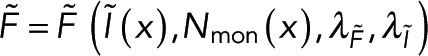
Equation 3 quantitatively links two measured quantities—the spectroscopy signal and the microscopy signal—through the parameter of interest,  . If the functional relationship between
  and
and  is experimentally measured and found to follow the form predicted by Eq. 3, then both Eqs. 1 and 2 would be validated. Because each pixel contains a measurement of the spectroscopy and microscopy signals, a single image produces many data points with which to test Eq. 3.
To calculate polymer amount at a specific location using both  and
and  , we combine Eqs. 1 and 2 to write
  in terms of the
  and
and  :
:
 (4) (4)
|
We will apply this approach to construct a system for measuring the amount of tubulin in polymer in cell extracts. We use fluorescence lifetime imaging microscopy (FLIM) for our spectroscopy technique to measure FRET—our spectroscopy signal. We use two-photon imaging as our microscopy technique to measure fluorescence intensity—our microscopy signal. Other microscopy or spectroscopy techniques could be used instead. In the next section, we present explicit models (i.e., write out the form of Eqs. 1 and 2 for our system) to construct a relationship between FRET and fluorescence intensity (i.e., Eq. 3 for our system) and the relationship between these measurements and polymer amount (i.e., Eq. 4 for our system). Then, in the following sections, we develop a quantitative means of measuring FRET using FLIM and experimentally test the relationship between FRET and intensity in cell extracts. In the final section, we experimentally test how well our system measures the amount of tubulin in polymer in a purified system.
Modeling the relationship between FRET, fluorescence intensity, and polymer
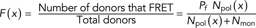
In this section, we present a model that relates the amount of tubulin assembled into microtubules to FRET and fluorescence intensity. We make several assumptions in the construction of the model, the validity of which will be tested based on the applicability of the model’s predictions to experimental data. We consider a scenario in which a fraction of tubulin molecules is labeled with a donor fluorophore, a fraction is labeled with an acceptor fluorophore, and the remaining tubulin molecules are unlabeled (Figure 1). When this mixture of tubulin is incorporated into a microtubule, we assume that, with some probability Pf, the donor-labeled tubulin neighbors an acceptor-labeled tubulin, allowing for FRET from the donor fluorophore to the acceptor fluorophore. We assume that FRET occurs only between tubulins in a microtubule and use the common two-state model for FRET (Cantor and Schimmel, 1980; Lakowicz, 2006; Mertz, 2010). At a specific location x, we call the fraction of donors engaged in FRET the “FRET fraction,” F, and relate it to the number of donor-labeled tubulins in monomer, Nmon, and the number of donor-labeled tubulins in polymer, Npol, by
 (5) (5)
|
FIGURE 1:
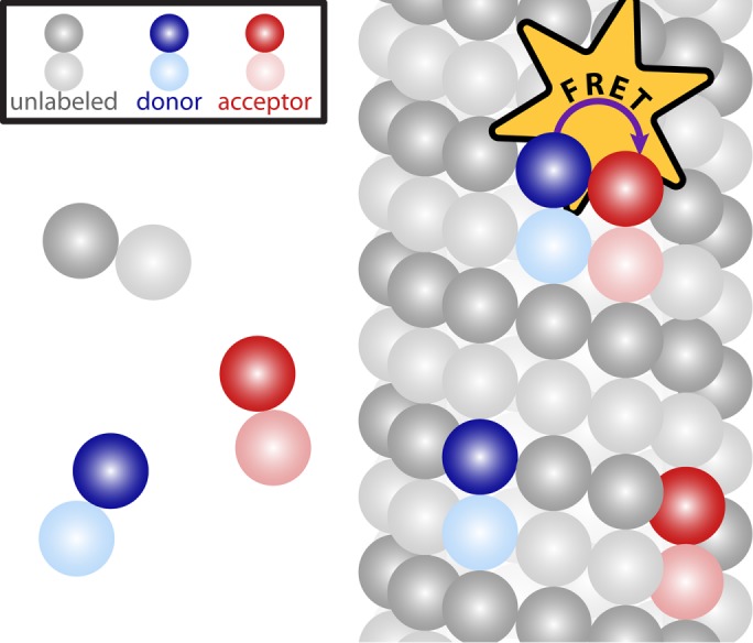
The assumed conditions for FRET. Some tubulin molecules are labeled with a donor fluorophore (blue), some are labeled with an acceptor fluorophore (red), and some are unlabeled (gray). We assume that FRET occurs only between a donor-labeled tubulin molecule and a nearby acceptor-labeled tubulin molecule in a microtubule, whereas tubulin molecules not incorporated in microtubules are not engaged in FRET.
We express Nmon(x) as Nmon because we assume the monomer concentration does not vary between locations. F is the realization of  , the spectroscopy signal; Pf is the realization of
  , an additional parameter that affects the spectroscopy signal; Eq. 5 is the realization of Eq. 1. The intensity, I, is defined as the photon generation rate of donors both engaged and not engaged in FRET per confocal volume:
|
|
where ε is the average number of photons detected per donor and α represents the relative brightness of donors engaged in FRET to donors not engaged in FRET. I is the realization of  , the microscopy signal; Pf, ε, and α are realizations of
  , the additional global parameters that affect the microscopy signal; Eq. 6 is the realization of Eq. 2. By solving for
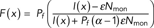
  in Eqs. 5 and 6, we obtain the relationship between FRET fraction, F, and intensity, I:
 (7) (7)
|
Equation 7 is the realization of Eq. 3 for this system. A single image provides many locations at which F(x) and I(x) have been measured. If the set of measured F(x) and I(x) agrees with Eq. 7, it not only validates Eqs. 5 and 6, from which Eq. 7 was derived, but it also allows the parameters  ,
,  , and α to be extracted from the fit. If the total concentration of donor in the sample is known (which sets the average value of
  ), then ε can be determined as well.
We combined Eqs. 5 and 6 to derive a formula for tubulin in polymer:
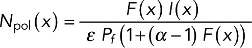 (8) (8)
|
which is the realization of Eq. 4. The average tubulin in polymer,  , can be found by averaging the amount of tubulin in polymer over the desired locations,
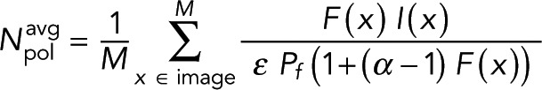 (9) (9)
|
where M is the number of locations. In this section, we applied the abstract formalism presented in the last section to a FRET-based measurement of polymer amount. In the next section, we construct a molecular FRET probe and test a model that relates fluorescence lifetime to FRET.
Measuring FRET and intensity
We use time-domain FLIM with two-photon microscopy to measure F(x) and I(x) (Eqs. 5 and 6). To make time-domain fluorescence measurements, a pulse of light is used to raise fluorophores into an excited state. Some of these fluorophores leave the excited state by emitting a photon (Figure 2A). These fluorophores stay in the excited state for a characteristic time called the fluorescence lifetime. By measuring the arrival times of these emitted photons relative to the excitation pulse, we can infer the fluorescence lifetime (Becker, 2010). If the fluorophore is a donor engaged in FRET, then the fluorescence lifetime of the donor fluorophore will be reduced because FRET provides an additional pathway for the donor to leave the excited state (Figure 2A). If there is a subpopulation of donors engaged in FRET and a subpopulation not engaged in FRET, we expect the measured fluorescence decay to be the sum of each subpopulation’s fluorescence decay. If we can measure the fraction of photons that came from a reduced-lifetime emission, then we can infer the fraction of donors engaged in FRET.
FIGURE 2:

Measuring FRET with FLIM. (A) Schematic diagram of excitation and relaxation pathways of the donor (blue) fluorophore. When a donor fluorophore absorbs an incoming photon, the fluorophore is raised into an excited state. The fluorophore relaxes back to the ground state by either emitting a photon or releasing heat. FRET introduces an additional nonradiative pathway for the fluorophore to relax. Thus, the average time the fluorophore spends in an excited state, referred to as the lifetime, is shorter when the fluorophore is engaged in FRET. (B) In purified solutions, in the absence of acceptor, fluorescence lifetime is not significantly affected by polymerization. Histogram of photon arrival times from Atto565-conjugated tubulin (donor-labeled tubulin) in Taxol-assembled microtubules (red dots) and without Taxol (blue dots). Bayesian analysis of these histograms using a single-exponential decay model estimates the fluorescence lifetimes (with Taxol; 3.45 ± 0.04 ns; without Taxol, 3.67 ± 0.03 ns) and provides the corresponding models (with Taxol, red curve; without Taxol, blue curve). (C) In purified solutions, Taxol-induced microtubules formed in the absence of an acceptor (green) produce a photon arrival time histogram that is a decaying exponential with a lifetime of ∼4 ns. FRET happens in the presence of acceptor fluorophore (purple), which induces the addition of a short component with a ∼1-ns lifetime.
Although the presence of FRET can lead to a dramatic reduction in the lifetime of a donor fluorophore, other changes in the local environment can also modify the fluorescence lifetime. To analyze the sensitivity of the lifetime of our donor fluorophore, Atto565-labeled tubulin, to changes in its local environment, we used a Bayesian approach to measuring lifetimes (Supplemental Materials). We first investigated the change in lifetime of Atto565-labeled tubulin in purified solutions before and after polymerization. FLIM measurements of 25 μM tubulin (with ∼1 in 20 tubulins labeled with Atto565) were fitted with a single-exponential model that determined a lifetime of 3.58 ± 0.03 ns for soluble tubulin and 3.45 ± 0.04 ns with tubulin polymerized with 20 μM Taxol (Figure 2B), where the error is the SD in the lifetimes between three different fields of view. This result demonstrates that incorporation into microtubules does not significantly change the lifetime of Atto565-labeled tubulin in buffer.
Next we examined whether the lifetime of Atto565-labeled tubulin changed after polymerization in Xenopus egg extracts. Bayesian analysis of FLIM measurements of 1.2 μM donor-labeled tubulin in extract gave a lifetime of 3.57 ± 0.03 ns. After assembly of microtubules with 1 μM Taxol, the analysis gave a lifetime of 3.50 ± 0.03 ns. Taken together, these control experiments argue that the lifetime of donor-labeled tubulin is not significantly altered by local environmental changes that occur during microtubule assembly in extract or buffer.
Next we tested whether donor-labeled tubulin could engage in FRET when coassembled into polymer with Atto647N-labeled tubulin, an acceptor. In the absence of acceptor, we induced 50 µM tubulin (with ∼1 in 4 tubulins labeled with Atto-565) to form microtubules in BRB80 with the addition of 10 µM Taxol. The histogram of photon arrival times was approximately a straight line on a semilog plot (Figure 2C, green curve), suggesting that our donor-labeled tubulin follows a monoexponential decay in the absence of acceptor. We then created a solution of 50 μM tubulin with both donor and acceptor (∼1 in 2 tubulins being acceptor labeled and ∼1 in 100 donor labeled) and formed microtubules using Taxol. We found the emergence of a short-lifetime decay in the histogram of photon arrival times (Figure 2C, purple curve). We attribute the short-lifetime decay to a subpopulation of donor-labeled tubulin engaged in FRET with acceptor-labeled tubulin and the long-lifetime decay component to a subpopulation of donor-labeled tubulin not engaged in FRET. To confirm that the short-lifetime decay was not due to additional, non-FRET contributions from the acceptor such as spectral bleedthrough, we repeated the measurement without the addition of Taxol. We found that in the absence of microtubules, the decay remained monoexponential (Figure 2C, orange curve). Taken together, these experiments argue that the observed short-lifetime decay is due to FRET between donor and acceptor incorporated into microtubules.
These results suggest that the photon emission is a sum of two exponentials:
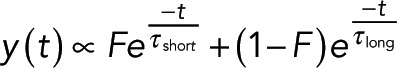 (10) (10)
|
where y(t) is the number of photons emitted at time t, F is the fraction of donors engaged in FRET, τshort is the lifetime of the donors that are engaged in FRET, and τlong is the lifetime of donors that are not engaged in FRET. We use Eq. 10 in our Bayesian analysis to estimate F(x) from the histogram of photon arrival times at each location x. To reduce the number of free parameters, we first obtain the lifetimes in control experiments (Materials and Methods). We estimate I(x) as the number of photons collected at location x corrected for stray light and detector dark noise (Materials and Methods).
Testing the FRET and intensity relationship in cell extracts
Next we tested our model for the relationship between FRET and intensity for microtubules assembled in cell extracts, which is the basis of our proposed method for measuring microtubule assembly. We first added 1.2 μM donor-labeled tubulin and 1.6 μM acceptor-labeled tubulin to Xenopus egg extract and induced microtubule formation with Taxol. An intensity image revealed that asters and other large assemblies of microtubules form within minutes of Taxol addition (Figure 3A), as observed previously (Verde et al., 1991; Foster et al., 2015). In each pixel, we estimated the fraction of donors engaged in FRET to create a FRET-fraction map, which displays similar spatial structure to the intensity image (Figure 3A). When Taxol is not added, and thus no microtubule assembly is induced, relatively little FRET is seen, and intensity images are uniform (Supplemental Figure S1).
FIGURE 3:

Investigating the relationship between FRET fraction and intensity. (A) An intensity image of microtubule structures in extract (left) and corresponding FRET-fraction map (right). (B) FRET fraction vs. intensity from the data in A for individual pixels (small blue dots) and grouped pixels (black dots). Error bars are the SD of the posterior distribution. The grouped pixels are well fitted by Eq. 7 (dark gray dashed line) with Pf = 0.123 ± 0.006 and  , where error is the 95% confidence interval.
To test the relationship between FRET fraction and intensity given by Eq. 7, we made a plot of FRET fraction versus intensity for every pixel (Figure 3B, blue dots). Although there appears to be a correlation between FRET fraction and intensity, the variance of these points is very large, presumably due to the low number of photons in each pixel. We therefore grouped pixels by intensity and then estimated the FRET fraction and average intensity from donors in each of these groups (Materials and Methods). Plotting the FRET fraction versus intensity of these grouped pixels revealed a clear trend (Figure 3B, black dots), which was well fitted by Eq. 7 (Figure 3B, dashed line), with best-fit values of Pf = 0.123 ± 0.006 and  , where α, the relative brightness of donors engaged in FRET to those not engaged in FRET, was previously estimated by the ratio of lifetimes as 0.45. The excellent fit of Eq. 7 demonstrates the ability of our model to describe the relationship between our microscopy and spectroscopy signals.
The parameters in our model—Pf and εNmon—are not arbitrary fitting parameters but correspond to physical quantities that can be varied. To further test our model, we varied experimental variables to see whether Pf and εNmon changed as expected. The first experimental variable we changed was acceptor concentration. Decreasing acceptor concentration from 1.3 to 0.6 μM resulted in similar intensity images and a global reduction in FRET fraction (Figure 4A). Grouping pixels as described and fitting Eq. 7 (Figure 4B) revealed that εNmon was similar (20.7 ± 3.5 and 16.4 ± 5.6, respectively), whereas Pf decreased from 0.107 ± 0.004 to 0.058 ± 0.004. Thus, as expected, changing acceptor concentration modified the probability of a donor-labeled tubulin in a microtubule engaging in FRET, Pf, without affecting the intensity from soluble monomers, εNmon. To see whether this trend continued, we titrated acceptor-labeled tubulin from 0 to 1.6 μM in increments of 0.32 μM and found that Pf scaled linearly with acceptor concentration (Figure 4C), whereas εNmon remained constant (Figure 4D). The observed linear relationship between Pf and acceptor concentration is expected in the low–acceptor concentration regime because the probability that at least one neighbor is an acceptor is equal to the fraction of tubulin that is acceptor labeled. The slope of Pf versus acceptor concentration is proportional to the number of neighbors with which a donor can FRET, which, after taking the endogenous tubulin concentration to be 18 μM (Parsons and Salmon, 1997), gives 1.84 ± 0.16 neighbors (Materials and Methods).
FIGURE 4:

Fit parameters change as expected when acceptor concentration is varied. (A) Intensity images (left) and FRET-fraction maps (right) of Taxol-induced microtubules in Xenopus egg extracts with high (top) and low (bottom) acceptor concentrations. FRET-fraction maps were sensitive to acceptor concentration, whereas the intensity images showed no significant differences. (B) Colored dots, FRET fraction and intensity from the data in A for grouped pixels. Error bars are the SD of the posterior distribution. The grouped pixels are well fitted by Eq. 7 (gray dashed lines) with Pf = 0.107 ± 0.004 and  for 1.3 μM acceptor, and Pf = 0.058 ± 0.004 and
  for 0.6 μM acceptor. Samples with more acceptor have a larger horizontal asymptote, leading to a larger Pf, the probability of FRET. Meanwhile, the x-intercept is unchanged, leading to
  , the number of photons from donor in monomer, being unchanged. (C) Black dots: Pf determined from model fitting as in B. Colored circles denote the Pf values from the best fit of data from samples in A and B. Error bars are 95% confidence intervals. Pf increases linearly with acceptor concentration (gray dashed line). (D) Black dots,
  , determined from model fitting as shown in B. Colored circles denote the
  values from the best fit of data from samples in A and B. Error bars are 95% confidence intervals.
  is unchanged when acceptor concentration is varied.
Because fewer photons are collected with shorter acquisition times, we expect εNmon to decrease with decreasing acquisition time. Fixing acceptor concentration (5 μM) and varying acquisition time from 50 to 10 s resulted in dimmer images but similar FRET fraction maps (Figure 5A). Grouping pixels as described and fitting Eq. 7 (Figure 5B) revealed that Pf was similar (0.330 ± 0.012 and 0.313 ± 0.031, respectively), whereas εNmon decreased from 76.4 ± 3.5 to 14.8 ± 1.9. We next systematically varied acquisition time from 5 to 50 s in intervals of 5 s and found that Pf did not significantly change with acquisition time, as expected, because Pf is a property of the sample, not acquisition parameters (Figure 5C), whereas εNmon increased linearly with acquisition time (Figure 5D). The linear relationship between εNmon and acquisition time is expected because the number of photons detected depends linearly on acquisition time. Thus both free parameters Pf and εNmon quantitatively varied as expected with changes in experimental conditions, supporting both the model described by Eqs. 5 and 6 and the accuracy of the experimental system.
FIGURE 5:

Fit parameters change as expected when acquisition time is varied. (A) Intensity images and FRET-fraction maps of Taxol-induced microtubules in Xenopus egg extracts acquired with a long (purple) and a short (green) acquisition time. Shorter acquisition times resulted in dimmer images but similar FRET-fraction maps. (B) Colored dots, FRET fraction and intensity from the data in A for grouped pixels. Error bars are the SD of the posterior distribution. The grouped pixels are well fitted by Eq. 7 (gray dashed line) with Pf = 0.330 ± 0.012 and  = 76.4 ± 3.5 for 50-s acquisition, and Pf = 0.313 ± 0.031 and
  = 14.8 ± 1.9 for 10-s acquisition. The x-intercept increases with acquisition time, leading to a larger
  . Meanwhile, the horizontal asymptote, which determines Pf, is unchanged. (C) Black dots, Pf determined from model fitting as shown in B. Colored circles denote the Pf values from the best fit of data from samples shown in A and B. Error bars are 95% confidence intervals. Pf is unchanged when acquisition time is varied (gray dashed line). (D) Black dots, determined from model fitting as in B. Colored circles denote the
  values from the best fit of data from samples in A and B. Error bars are 95% confidence intervals.
  increases linearly with acquisition time (gray dashed line).
Measuring polymer concentration
After validating the FRET and intensity measurements of microtubules, we next sought to test whether this assay could accurately determine polymer concentration. To do this, we created three dilution series of Taxol-stabilized microtubules with 8.3% donor-labeled tubulin, 16.7% acceptor-labeled tubulin, and 75% unlabeled tubulin in BRB80. To find ε, we first created a sample containing 50 µM tubulin and measured Pf and εNmon by fitting Eq. 7 to the FRET fraction and the intensity of grouped pixels (as described). Using these values, we then calculated εNpol with Eq. 9. We divided the sum of εNpol and εNmon by the known tubulin concentration to obtain ε in units of photons per micromolar of tubulin.
The amount of polymer was measured in six fields of view for each sample in the microtubule dilution series by finding Pf and εNmon by fitting Eq. 7 to the FRET fraction and the intensity of grouped pixels (as described). We then calculated the polymer concentration in each field of view with Eq. 9. The polymer concentration, when averaged over fields of view, was similar to the tubulin concentration for the entire dilution series (Figure 6, green dots). This was expected due to the high molarity of Taxol, which causes the majority of tubulin to be in polymer. To compare our methodology to an established technique, we then recreated in triplicate the microtubule dilution series without labeled tubulin. The dilution series was centrifuged and solubilized, and the pellet was depolymerized in ice-cold BRB80. We then measured the concentration of tubulin by 280-nm absorption three times for each sample (Figure 6, blue dots). Our measurement was in good agreement with the polymer concentration measured using ultracentrifugation. Unlike ultracentrifugation, which provides a measurement of polymer averaged across a sample, our measurements are spatially resolved. To illustrate this advantage, we calculated the polymer concentration at each location within a field of view using Eq. 8 (Figure 6, inset). These results, in conjunction with our previous findings, illustrate how our methodology can be used to construct time-resolvable, nondestructive assays that faithfully measure polymer concentration.
FIGURE 6:
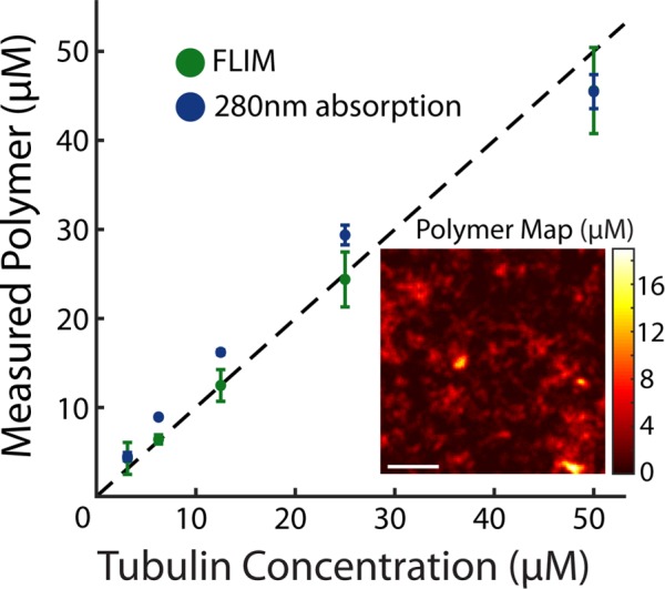
Microtubule dilution series to test measurements of polymer concentration. Polymer measurements by FRET-intensity (green dots) and centrifugation followed by absorption at 280 nm (blue dots) correspond to the expected polymer amount (black dashed line). Error bars are SEM. Inset, map of the concentration of tubulin subunits in polymer. Scale bar, 25 μm.
Testing the methodology in cells
We next tested how the methodology could be applied to another system: FRET measurements of spindles in cells. To obtain cells with fluorescently labeled tubulin, we created a stable cell line of U2OS cells expressing SNAP-tag-α-tubulin and incubated these cells with JF549-cpSNAP-tag, our donor fluorophore, and JF646-SNAP-tag, our acceptor fluorophore (Materials and Methods). We performed FLIM measurements on mitotic cells, revealing spindles when viewed with two-photon intensity imaging (Figure 7). We then segmented the image to include only the spindle region and found the lifetimes of donors engaged in FRET and not engaged in FRET (Materials and Methods). We grouped pixels as described earlier and saw a clear relationship between FRET fraction and intensity (Figure 7, purple dots), which was well fitted by Eq. 7 (Figure 7B, purple dashed line), with best-fit values of Pf = 0.091 ± 0.008 and εNmon = 19.9 ± 4.6, where α, the relative brightness of donors engaged in FRET to those not engaged in FRET, was previously estimated by the ratio of lifetimes. The fit of Eq. 7 demonstrates the ability of the model to describe the relationship between FRET and intensity within subcellular structures in these cells. In the absence of acceptor, the measured FRET fraction was drastically reduced, and this relationship disappeared (Figure 7B, green dots), arguing that the measured FRET was due to FRET from donor- to acceptor-labeled tubulin. We next sought to use this method to measure the concentration of microtubules in spindles by applying Eq. 9. This procedure requires measuring ε. To find ε in units of photons per micromolar tubulin, we use the fact that tubulin must be in either monomer or polymer; thus
where  is the total number density, or total concentration, of tubulin. Combining this equation with Eqs. 5 and 6 gives
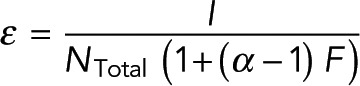 |
FIGURE 7:
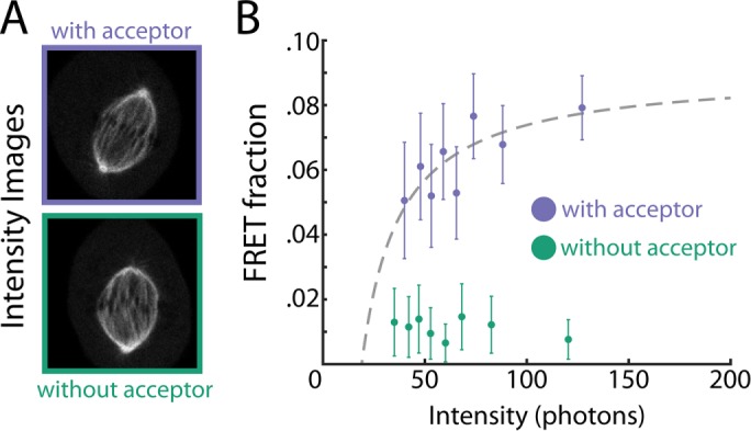
Investigating the relationship between FRET fraction and intensity in U2OS cells. (A) An intensity image of a mitotic spindle from a cell with both donor- and acceptor-labeled tubulin (top) and from a cell with only donor-labeled tubulin (bottom). (B) Colored dots, FRET fraction and intensity from the data in A for grouped pixels. Error bars are the SD of the posterior distribution. The grouped pixels from the sample with both donor and acceptor is well fitted by Eq. 7 (gray dashed lines) with Pf = 0.091 ± 0.008 and  , where error is the 68% confidence interval.
This equation holds true for any volume. NTotal averaged over the cell has been reported to be 20 µM (Hiller and Weber, 1978). Combining this value with measurements of FRET fraction, F, and intensity, I, averaged over the cell allowed us to calculate ε in an individual cell. We then segmented the spindle from the image and found Pf by fitting Eq. 7 to FRET fraction and intensity of grouped pixels. We use these values in Eq. 9 to estimate the microtubule concentration to be 39 ± 3 µM in the spindle, where the error is the SD between cells (n = 6). These results show the applicability of the methodology in both cell extracts and cells.
DISCUSSION
Time-resolvable quantitative measurements of polymer concentration are very useful for studying protein polymerization pathways. It is difficult to construct such quantitative readouts of polymer in cells and cell extracts. Although fluorescence microscopy and spectroscopy methods are often used to measure polymer amount, fluorescence microscopy can be insensitive to polymer amount for early time points after nucleation when polymers are small, whereas spectroscopy measurements can be hard to interpret and are subject to many artifacts. We developed a methodology to use microscopy and spectroscopy measurements simultaneously to overcome the limitations of both approaches in cells and cell extracts.
First, we constructed a model that describes how the intensity and FRET fraction depend on the partitioning of subunits into monomer and polymer. The model predicts that FRET and intensity are related to each other due to the presence of polymer (Eq. 7). We then used a combination of two-photon microscopy with FLIM to simultaneously measure intensity—our microscopy signal—and FRET—our spectroscopy signal—at each pixel in an image. We then grouped these pixels to test the relation between FRET fraction and intensity and found that Eq. 7 described the data remarkably well. This supports the validity of each of the measurements. We also observed that the best-fit values of the two free parameters quantitatively changed as expected with changes in the experimental variables. We then showed that our combined microscopy–spectroscopy technique recapitulated the average measurements of ultracentrifugation while providing spatially resolved measurements. We applied our methodology to validate a new polymer measurement system in cells. Finally, we applied this measurement system to estimate the microtubule concentration within a subcellular structure: the spindle.
We used approximations to make a tractable model, including a two-state model for FRET, that all donors in polymer are equally likely to FRET and that the fraction of donors engaged in FRET is linearly related to the amount of polymer. The net effect of our approximations is presumably very small, as suggested by the quantitative agreement between the model and the data under many different conditions. Use of simplifying assumptions reduces the number of free parameters, allowing for testing of the model with data without overfitting.
A unique advantage of this method is the cross-validation of the spectroscopy measurement and the microscopy measurement. In cells, it is challenging to precisely control the acceptor concentration, and changes in acceptor concentration can vary how FRET relates to polymer. Simultaneous measurements of FRET and intensity allow this difficulty to be overcome by cross-validation in each cell. Another advantage of combining microscopy and spectroscopy measurements is that the resulting polymer measurement has a broader range of sensitivity. The microscopy measurement is sensitive to the change in polymer amount in the high-polymer regime. This is because intensity increases linearly with the amount of polymer in the high-polymer limit. However, due to the presence of soluble subunits, the fractional change in intensity is small in the low-polymer regime. On the other hand, polymer measurements by FRET are sensitive to the change in polymer amount in the low-polymer regime. FRET fraction linearly increases with the polymer amount in the low-polymer limit. However, FRET only marginally changes in the high-polymer regime because in this limit, large changes in the amount of polymer correspond to small changes in the fraction of subunits in polymer (which, by construction, cannot exceed 1). Therefore, combining two measurements enables us to measure changes in polymer amount both in the high- and low-polymer regimes.
In summary, we combined microscopy and spectroscopy measurements to build a novel system for collecting microtubule polymerization curves in cell extracts. This methodology can be applied to any protein complex and any set of spectroscopy and microscopy measurements. Here we used two-photon microscopy, but other microscopy methods, such as total internal reflection fluorescence or superresolution microscopy, can be used. Although FRET was used in this study, other spectroscopy signals, such as steady-state anisotropy for measuring rotational diffusion times or homo-FRET, can be used. Our method is particularly well suited for experiments requiring high temporal resolution, as in polymerization curve measurements, high spatial resolution, as in subcellular measurements, or nondestructive measurements—for example, if a single cell time course is required. We hope that this framework will allow researchers to develop new quantitative polymer assays to study other polymer assembly pathways.
MATERIALS AND METHODS
Sample preparation
Samples were observed in a conventional flow cell. Bovine tubulin was purified and labeled with fluorophores as previously described (Mitchison and Kirschner 1984; Mitchison, 2012; Hyman et al., 1991). Cytostatic factor–arrested egg extracts were prepared from X. laevis oocytes as described previously (Hannak and Heald, 2006). Tubulin was polymerized in egg extracts by adding donor labeled tubulin to 1.2 μM and Taxol (in dimethyl sulfoxide [DMSO]) to 5 μM at room temperature unless otherwise noted.
To make microtubule dilution series, we mixed unlabeled and labeled tubulin together in BRB80 with 1 mM dithiothreitol (DTT) and 1 mM GTP. This was incubated on ice for 5 min before 1/10 volume of 1 μM Taxol per μM tubulin was slowly added. This mixture was then incubated at 37°C for 10 min before 1/10 volume of 10 μM Taxol per μM tubulin was slowly added. This mixture was then incubated at 37°C for 10 min. To create the microtubule dilution series, the polymer solution was diluted by factors of two into polymerization buffer, which is composed of 50 μM Taxol, 10% DMSO (vol/vol), 1 mM DTT, 1 mM GTP, and BRB80.
U2OS cell lines were maintained in DMEM (Life Technologies) supplemented with 10% fetal bovine serum (Life Technologies) and 50 IU/ml penicillin and 50 μg/ml streptomycin (Life Technologies) at 37°C in a humidified atmosphere with 5% CO2. A stable U2OS cell line expressing SNAP-tag-α-tubulin was generated through a retroviral transfection with 200 μg/ml hygromycin (Life Technologies) selection. For live-cell imaging, cells were grown on a 25-mm-diameter, #1.5-thickness, circular coverglass coated with poly-d-lysine (GG-25-1.5-pdl; neuVitro) to 80–90% confluency. To associate SNAP-tag-α-tubulin with fluorescent SNAP-tag ligands, the cells were incubated for 30 min with 150 nM JF549-cpSNAP-tag for negative control experiments or with both 150 nM JF549-cpSNAP-tag and 1350 nM JF646-SNAP-tag ligands for FRET experiments, followed by three washes with DMEM (Grimm et al., 2015). Then the cells were incubated in imaging medium, which is FluoroBrite DMEM (Life Technologies) supplemented with 4 mM l-glutamine (Life Technologies) and 10 mM 4-(2-hydroxyethyl)-1-piperazineethanesulfonic acid, for ∼15–30 min before imaging. The coverglass was mounted on a custom-built temperature controlled microscope chamber at 37°C, and covered with 1.5 ml of imaging media and 2 ml of white mineral oil (VWR). An objective heater (Bioptech) was used to maintain the objective at 37°C.
Microscopy
Our microscope system was constructed around an inverted microscope (Eclipse Ti; Nikon, Tokyo, Japan), with a Ti:sapphire pulsed laser (Mai-Tai; Spectra-Physics, Mountain View, CA) for two-photon excitation (1000-nm wavelength, 80-MHz repetition rate, ∼70-fs pulse width), a commercial scanning system (DCS-120; Becker & Hickl, Berlin, Germany), and hybrid detectors (HPM-100-40; Becker & Hickl). The excitation laser was collimated by a telescope assembly to fully utilize the numerical aperture (NA) of a water-immersion objective (CFI Apo 40 WI, NA 1.25; Nikon) and avoid power loss at the XY galvanometric mirror scanner. The fluorescence from samples was imaged with a nondescanned detection scheme with a dichroic mirror (705 LP; Semrock) that was used to allow the excitation laser beam to excite the sample while allowing fluorescent light to pass into the detector path. A short-pass filter was used to further block the excitation laser beam (720 SP; Semrock), followed by an emission filter appropriate for Atto565-labeled tubulin (590/30 nm BP; Semrock).
Photon arrival time histograms
We use a Becker and Hickl Simple-Tau 150 FLIM system to record photon arrival time histograms. All arrival times are measured relative to the excitation of a photodiode that is triggered by the excitation laser (Becker, 2010). The TAC range was set to 7 × 10⁻⁸, with a gain of 5, corresponding to a 14-ns maximum arrival time. The TCSPC system can lose fidelity for photons that arrive just before or after the excitation of the photodiode (Becker, 2010), and thus we set the lower and upper limits to 10.59 and 77.25, respectively, resulting in an ∼10-ns recording interval. The instrument response function was measured using fixed-point illumination of second harmonic generation of a urea crystal. For most measurements, the intensity of the illumination beam was set such that there were ∼100,000 photons/s recorded. Data were acquired as a 128 × 128 pixel image, where a corresponding photon arrival time histogram was recorded for each pixel.
Polymer measurements by absorption
Tubulin concentration was determined using a NanoDrop spectrophotometer with an extinction coefficient of 1.15 (mg/ml)–1 cm–1 (Widlund et al., 2012.
Data analysis
Estimating the FRET fraction and intensity from photon arrival histograms.
We used a Bayesian model to build posterior distributions from photon arrival time histograms (Supplemental Materials). The posterior was evaluated at uniformly spaced grid points in parameter space. Point estimates of the FRET fraction were found by taking the maximum of the posterior distribution of the FRET fraction. To reduce the number of free parameters when analyzing photon arrival histograms to find the FRET fraction, we first found the two lifetimes of the donor fluorophore and then fixed those lifetimes in our Bayesian analysis. This reduced the number of free parameters from four to two. Intensity is defined as the number of photons from donors per pixel per acquisition. The number of photons from donors is found by taking the product of the number of photons and the expected value of the fraction of photons from donors.
We used the following procedure to find lifetimes in each day’s freshly prepared extract and U2OS cells and for our experiments in buffer. To find  , the lifetime from donors not engaged in FRET, we measured a sample that had no acceptor-labeled tubulin (i.e., no FRET), and then used a single-exponential decay model in our Bayesian analysis to find the maximum a posteriori estimate lifetime. Then we measured a sample that had both donor and acceptor in microtubules, fixing the newly found
  and built a posterior distribution on the fraction of photons from donors engaged in FRET and not engaged in FRET and the lifetime of donors engaged in FRET (
 ). The maximum a posteriori estimate was used as the point estimate for the value of
  . These estimates of lifetimes were then used in the analysis for all measurements performed on that day’s extract. For cell data, only FLIM decays from the spindle region were used to determine lifetimes. To analyze FLIM decay curves from only the spindle region, we applied the Gaussian blur function from MATLAB, followed by thresholding to the intensity image. The resulting image was used as a mask for the original FLIM data.
For FRET fraction measurements in extract, we remove the first 0.6 ns from the photon arrival time histograms—as measured from the maximum of the photon arrival time histogram—to filter out very short lifetime photons that come from endogenous fluorescence. Because our model does not consider the time decay of extract fluorescence, removing early time bins makes the data more consistent with our model, which assumes that photons come only from donors and stray light and detector dark noise (Supplemental Materials). For FRET fraction measurements in buffer, we remove the first 0.2 ns.
Fit parameters and error bars.
For Figures 3B, 4B, 5B, and 7B, error bars are 68.2% credible intervals. To obtain best-fit parameters and confidence intervals, we used the weighted fit function from MATLAB to fit Eq. 7, where the weights are the inverse of the SD of the posterior distribution of the FRET fraction. Reported errors in the best-fit values of the parameters are the 95% confidence intervals, except for Figure 7B, which uses a 68% confidence interval. For Figures 4, C and D, and 5, C and D, we used the weighted fit function from MATLAB, where the weights are the square of the inverse of the SD, where SD was estimated as half of the 68.2% confidence interval. The error bars in Figure 6 are estimated as the SEM from three different microtubule dilution series, where polymer amount was measured three times for each sample using 280-nm absorption and in six fields of view for each sample in FRET-intensity measurements.
Constructing intensity images and FRET fraction and polymer maps.
For Figures 3A and 4A, the photon arrival time histograms of 10 consecutive 20-s acquisitions were summed at each pixel. To boxcar average each pixel, we summed the photon arrival time histogram at each pixel with the closest 24 pixels. We then applied our Bayesian analysis on the resulting photon arrival time histogram to find the FRET fraction at each boxcar-averaged pixel and the fraction of total photons that came from donors. The intensity map was created by dividing the total number of photons in the boxcar-averaged pixel by the number of pixels used in the boxcar average (25) and the number of acquisitions (10 for Figures 3A and 4A, and 1 for Figure 5A). For the polymer map presented in the inset of Figure 6, we boxcar averaged each pixel with the closest 8 pixels.
Grouping pixels.
Pixels were sorted by photon counts into pixel groups, where each pixel group is composed of the same number of pixels. The photon arrival time histogram for the pixel group was constructed by adding the histograms of each pixel in the group. To avoid bias due to low photon counts, no pixel group has <10,000 photons.
Supplementary Material
Acknowledgments
B.K. thanks the FAS Division of Science, Research Computing Group at Harvard University, for helping us use the Odyssey cluster for FLIM analysis. We thank the Lavis lab (Janiela Research Campus) for the generous gift of JF-SNAP-tag ligands. We also thank Ethan Garner, Jess Crossno, Daniel Walsh, Emily Davis, Julia Schwartzman, Zain Ali, and Lukas Bane for inspiration and thoughtful discussions. B.K. was supported by National Science Foundation GRFP Fellowship DGE1144152. T.Y. is grateful for a Samsung scholarship. This work was supported by National Science Foundation Grants PHY-0847188, PHY-1305254, and DMR-0820484.
Abbreviations used:
- FLIM
fluorescence lifetime imaging microscopy
- FRET
Förster resonance energy transfer.
Footnotes
This article was published online ahead of print in MBoC in Press (http://www.molbiolcell.org/cgi/doi/10.1091/mbc.E16-05-0344) on March 29, 2017.
REFERENCES
Boldface names denote co–first authors.
- Bastiaens PI, Squire A. Fluorescence lifetime imaging microscopy: spatial resolution of biochemical processes in the cell. Trends Cell Biol. 1999;9:48–52. doi: 10.1016/s0962-8924(98)01410-x. [DOI] [PubMed] [Google Scholar]
- Becker W. The bh TCSPC Handbook. Berlin: Becker and Hickl; 2010. [Google Scholar]
- Bordas J, Mandelkow EM, Mandelkow E. Stages of tubulin assembly and disassembly studied by time-resolved synchrotron X-ray scattering. J Mol Biol. 1983;164:89–135. doi: 10.1016/0022-2836(83)90089-x. [DOI] [PubMed] [Google Scholar]
- Cantor CR, Schimmel PR. Biophysical Chemistry. Part 2: Techniques for the Study of Biological Structure and Function. New York: W. H. Freeman and Company; 1980. [Google Scholar]
- Cooper JA, Buhle EL, Walker SB, Tsong TY, Pollard TD. Kinetic evidence for a monomer activation step in actin polymerization. Biochemistry. 1983;22:2193–2202. doi: 10.1021/bi00278a021. [DOI] [PubMed] [Google Scholar]
- Cooper JA, Pollard TD. Methods to measure actin polymerization. Methods Enzymol. 1982;82:182–210. doi: 10.1016/0076-6879(82)85021-0. [DOI] [PubMed] [Google Scholar]
- Cox MM. Historical overview: searching for replication help in all of the rec places. Proc Natl Acad Sci USA. 2001;98:8173–8180. doi: 10.1073/pnas.131004998. [DOI] [PMC free article] [PubMed] [Google Scholar]
- Desai A, Mitchison TJ. Microtubule polymerization dynamics. Cell Dev Biol. 1997;13:83–117. doi: 10.1146/annurev.cellbio.13.1.83. [DOI] [PubMed] [Google Scholar]
- Dokland T. Freedom and restraint: themes in virus capsid assembly. Structure. 2000;8:157–162. doi: 10.1016/s0969-2126(00)00181-7. [DOI] [PubMed] [Google Scholar]
- Fletcher DA, Mullins RD. Cell mechanics and the cytoskeleton. Nature. 2010;463:485–492. doi: 10.1038/nature08908. [DOI] [PMC free article] [PubMed] [Google Scholar]
- Flyvbjerg H, Jobs E, Leibler S. Kinetics of self-assembling microtubules: an “inverse problem” in biochemistry. Proc Natl Acad Sci USA. 1996;93:5975–5979. doi: 10.1073/pnas.93.12.5975. [DOI] [PMC free article] [PubMed] [Google Scholar]
- Foster PJ, Fürthauer S, Shelley MJ, Needleman DJ. Active contraction of microtubule networks. Elife. 2015;4:e10837. doi: 10.7554/eLife.10837. [DOI] [PMC free article] [PubMed] [Google Scholar]
- Frieden C. Polymerization of actin: mechanism of the Mg2+-induced process at pH 8 and 20°C. Proc Natl Acad Sci USA. 1983;80:6513–6517. doi: 10.1073/pnas.80.21.6513. [DOI] [PMC free article] [PubMed] [Google Scholar]
- Frieden C. Actin and tubulin polymerization: the use of kinetic methods to determine mechanism. Annu Rev Biophys Biophys Chem. 1985;14:189–210. doi: 10.1146/annurev.bb.14.060185.001201. [DOI] [PubMed] [Google Scholar]
- Frieden C, Goddette DW. Polymerization of actin and actin-like systems: evaluation of the time course of polymerization in relation to the mechanism. Biochemistry. 1983;22:5836–5843. doi: 10.1021/bi00294a023. [DOI] [PubMed] [Google Scholar]
- Garner EC, Campbell CS, Mullins RD. Dynamic instability in a DNA-segregating prokaryotic actin homolog. Science. 2004;306:1021–1025. doi: 10.1126/science.1101313. [DOI] [PubMed] [Google Scholar]
- Grimm JB, English BP, Chen J, Slaughter JP, Zhang Z, Revyakin A, Patel R, Macklin JJ, Normanno D, Singer RH, et al. A general method to improve fluorophores for live-cell and single-molecule microscopy. Nat Methods. 2015;12:244–250. doi: 10.1038/nmeth.3256. [DOI] [PMC free article] [PubMed] [Google Scholar]
- Hannak E, Heald R. Investigating mitotic spindle assembly and function in vitro using Xenopus laevis egg extracts. Nat Protocols. 2006;1:2305–2314. doi: 10.1038/nprot.2006.396. [DOI] [PubMed] [Google Scholar]
- Helmke KJ, Heald R. TPX2 levels modulate meiotic spindle size and architecture in Xenopus egg extracts. J Cell Biol. 2014;206:385–393. doi: 10.1083/jcb.201401014. [DOI] [PMC free article] [PubMed] [Google Scholar]
- Hiller G, Weber K. Radioimmunoassay for tubulin: a quantitative comparison of the tubulin content of different established tissue culture cells and tissues. Cell. 1978;14:795–804. doi: 10.1016/0092-8674(78)90335-5. [DOI] [PubMed] [Google Scholar]
- Hyman A, Drechsel D, Kellogg D, Salser S, Sawin K, Steffen P, Wordeman L, Mitchison TJ. Preparation of modified tubulins. Methods Enzymol. 1991;196:478–485. doi: 10.1016/0076-6879(91)96041-o. [DOI] [PubMed] [Google Scholar]
- Katen S, Zlotnick A. The thermodynamics of virus capsid assembly. Methods Enzymol. 2009;455:395–417. doi: 10.1016/S0076-6879(08)04214-6. [DOI] [PMC free article] [PubMed] [Google Scholar]
- Kaye B, Foster PJ, Yoo TY, Needleman DJ. Developing and testing a Bayesian analysis of fluorescence lifetime measurements. PLoS One. 2017;12:e0169337. doi: 10.1371/journal.pone.0169337. [DOI] [PMC free article] [PubMed] [Google Scholar]
- Lakowicz JR. Principles of Fluorescence Spectroscopy. New York: Springer; 2006. [Google Scholar]
- Matsudaira P, Bordas J, Koch MH. Synchrotron x-ray diffraction studies of actin structure during polymerization. Proc Natl Acad Sci USA. 1987;84:3151–3155. doi: 10.1073/pnas.84.10.3151. [DOI] [PMC free article] [PubMed] [Google Scholar]
- Mertz J. Introduction to Optical Microscopy. Greenwood Village, CO: Roberts and Company; 2010. [Google Scholar]
- Meyer RR, Laine PS. The single-stranded DNA-binding protein of Escherichia coli. Microbiol Rev. 1990;54:342–380. doi: 10.1128/mr.54.4.342-380.1990. [DOI] [PMC free article] [PubMed] [Google Scholar]
- Mitchison T, Kirschner M. Microtubule assembly nucleated by isolated centrosomes. Nature. 1984;312:232–237. doi: 10.1038/312232a0. [DOI] [PubMed] [Google Scholar]
- Mitchison T. Labeling tubulin and quantifying labeling stoichiometry. 2012. Available at https://mitchison.hms.harvard.edu/files/mitchisonlab/files/labeling_tubulin_and_quantifying_labeling_stoichiometry.pdf (accessed 22 May 2015)
- Mullins DR, Heuser JA, Pollard TD. The Interaction of Arp2/3 complex with actin: nucleation, high affinity pointed end capping, and formation of branching networks of filaments. Proc Natl Acad Sci USA. 1998;95:6181–6186. doi: 10.1073/pnas.95.11.6181. [DOI] [PMC free article] [PubMed] [Google Scholar]
- O’Connell JD, Zhao A, Ellington AD, Marcotte EM. Dynamic reorganization of metabolic enzymes into intracellular bodies. Cell Dev Biol. 2012;28:89–111. doi: 10.1146/annurev-cellbio-101011-155841. [DOI] [PMC free article] [PubMed] [Google Scholar]
- Ohba T, Nakamura M, Nishitani H, Nishimoto T. Self-organization of microtubule asters induced in Xenopus egg extracts by GTP-bound Ran. Science. 1999;284:1356–1358. doi: 10.1126/science.284.5418.1356. [DOI] [PubMed] [Google Scholar]
- Okamoto K, Hayashi Y. Visualization of F-actin and G-actin equilibrium using fluorescence resonance energy transfer (FRET) in cultured cells and neurons in slices. Nat Protocols. 2006;1:911–919. doi: 10.1038/nprot.2006.122. [DOI] [PubMed] [Google Scholar]
- Oosawa F, Kasai M. A theory of linear and helical aggregations of macromolecules. J Mol Biol. 1962;4:10–21. doi: 10.1016/s0022-2836(62)80112-0. [DOI] [PubMed] [Google Scholar]
- Parsons SF, Salmon ED. Microtubule assembly in clarified Xenopus egg extracts. Cell Motil Cytoskeleton. 1997;36:1–11. doi: 10.1002/(SICI)1097-0169(1997)36:1<1::AID-CM1>3.0.CO;2-E. [DOI] [PubMed] [Google Scholar]
- Petrovska I, Nüske E, Munder MC, Kulasegaran G, Malinovska L, Kroschwald S, Richter D, Fahmy K, Gibson K, Verbavatz JM, Alberti S. Filament formation by metabolic enzymes is a specific adaptation to an advanced state of cellular starvation. Elife. 2014;3:e02409. doi: 10.7554/eLife.02409. [DOI] [PMC free article] [PubMed] [Google Scholar]
- Pollard TD. Actin. Curr Opin Cell Biol. 1990;2:33–40. doi: 10.1016/s0955-0674(05)80028-6. [DOI] [PubMed] [Google Scholar]
- Pollard TD, Cooper JA. Actin and actin-binding proteins. A critical evaluation of mechanisms and functions. Annu Rev Biochem. 1986;55:987–1035. doi: 10.1146/annurev.bi.55.070186.005011. [DOI] [PubMed] [Google Scholar]
- Rohatgi R, Nollau P, Ho HY, Kirschner MW, Mayer BJ. Nck and phosphatidylinositol 4,5-bisphosphate synergistically activate actin polymerization through the N-WASP-Arp2/3 pathway. J Biol Chem. 2001;276:26448–26452. doi: 10.1074/jbc.M103856200. [DOI] [PubMed] [Google Scholar]
- Rowley MI, Barber PR, Coolen AC, Vojnovic B. Bayesian analysis of fluorescence lifetime imaging data. In: Proceedings SPIE 7903, Multiphoton Microscopy in the Biomedical Sciences XI, Bellingham, WA: SPIE, 790325. 2011.
- Rowley MI, Coolen ACC, Vojnovic B, Barber PR. Robust bayesian fluorescence lifetime estimation, decay model selection and instrument response determination for low-intensity FLIM imaging. PLoS One. 2016;11:e0158404. doi: 10.1371/journal.pone.0158404. [DOI] [PMC free article] [PubMed] [Google Scholar]
- Sept D, McCammon JA. Thermodynamics and kinetics of actin filament nucleation. Biophys J. 2001;81:667–674. doi: 10.1016/S0006-3495(01)75731-1. [DOI] [PMC free article] [PubMed] [Google Scholar]
- Taylor DL, Reidler J, Spudich JA, Stryer L. Detection of actin assembly by fluorescence energy transfer. J Cell Biol. 1981;89:362–367. doi: 10.1083/jcb.89.2.362. [DOI] [PMC free article] [PubMed] [Google Scholar]
- Tellam R, Frieden C. Cytochalasin D and platelet gelsolin accelerate actin polymer formation. A model for regulation of the extent of actin polymer formation in vivo. Biochemistry. 1982;21:3207–3214. doi: 10.1021/bi00256a027. [DOI] [PubMed] [Google Scholar]
- Tobacman LS, Korn ED. The kinetics of actin nucleation and polymerization. J Biol Chem. 1983;258:3207–3214. [PubMed] [Google Scholar]
- Verde F, Berrez JM, Antony C, Karsenti E. Taxol-induced microtubule asters in mitotic extracts of Xenopus eggs: requirement for phosphorylated factors and cytoplasmic dynein. J Cell Biol. 1991;112:1177–1187. doi: 10.1083/jcb.112.6.1177. [DOI] [PMC free article] [PubMed] [Google Scholar]
- Voter WA, Erickson HP. The kinetics of microtubule assembly. Evidence for a two-stage nucleation mechanism. J Biol Chem. 1984;259:10430–10438. [PubMed] [Google Scholar]
- Wang YL, Taylor DL. Probing the dynamic equilibrium of actin polymerization by fluorescence energy transfer. Cell. 1981;27:429–436. doi: 10.1016/0092-8674(81)90384-6. [DOI] [PubMed] [Google Scholar]
- Wegner A, Engel J. Kinetics of the cooperative association of actin to actin filament. Biophys Chem. 1975;3:215–225. doi: 10.1016/0301-4622(75)80013-5. [DOI] [PubMed] [Google Scholar]
- Wen KK, Rubenstein PA. Differential regulation of actin polymerization and structure by yeast formin isoforms. J Biol Chem. 2009;284:16776–16783. doi: 10.1074/jbc.M109.006981. [DOI] [PMC free article] [PubMed] [Google Scholar]
- Widlund PO, Podolski M, Reber S, Alper J, Storch M, Hyman A, Howard J, Drechel D. One-step purification of assembly-competent tubulin from diverse eukaryotic sources. Mol Biol Cell. 2012;23:4394–4401. doi: 10.1091/mbc.E12-06-0444. [DOI] [PMC free article] [PubMed] [Google Scholar]
- Wiese C, Wilde A, Moore MS, Adam SA, Merdes A, Zheng Y. Role of importin-beta in coupling Ran to downstream targets in microtubule assembly. Science. 2001;291:653–656. doi: 10.1126/science.1057661. [DOI] [PubMed] [Google Scholar]
- Zlotnick A, Johnson JM, Wingfield PW, Stahl SJ, Endres D. A theoretical model successfully identifies features of hepatitis B virus capsid assembly. Biochemistry. 1999;38:14644–14652. doi: 10.1021/bi991611a. [DOI] [PubMed] [Google Scholar]
Associated Data
This section collects any data citations, data availability statements, or supplementary materials included in this article.