Effective and extensible feature extraction method using genetic algorithm-based frequency-domain feature search for epileptic EEG multiclassification

Abstract

In this paper, genetic algorithm-based frequency-domain feature search (GAFDS) method is proposed for the electroencephalogram (EEG) analysis of epilepsy. In this method, frequency-domain features are first searched and then combined with nonlinear features. Subsequently, these features are selected and optimized to classify EEG signals. The extracted features are analyzed experimentally. The features extracted by GAFDS show remarkable independence, and they are superior to the nonlinear features in terms of the ratio of interclass distance and intraclass distance. Moreover, the proposed feature search method can search for features of instantaneous frequency in a signal after Hilbert transformation. The classification results achieved using these features are reasonable; thus, GAFDS exhibits good extensibility. Multiple classical classifiers (i.e., k-nearest neighbor, linear discriminant analysis, decision tree, AdaBoost, multilayer perceptron, and Naïve Bayes) achieve satisfactory classification accuracies by using the features generated by the GAFDS method and the optimized feature selection. The accuracies for 2-classification and 3-classification problems may reach up to 99% and 97%, respectively. Results of several cross-validation experiments illustrate that GAFDS is effective in the extraction of effective features for EEG classification. Therefore, the proposed feature selection and optimization model can improve classification accuracy.

1. Introduction

Epilepsy is a chronic disease characterized by a sudden abnormal discharge of brain neurons. In 2013, over 50 million patients were afflicted with epilepsy worldwide, with most patients originating from developing countries.^[1] Approximately 9 million epileptic patients were recorded in China in 2011. Every year, 600,000 new epileptic patients are recorded.^[2] In China, epilepsy has become the second most common nerve disease, coming in second to headache. Therefore, the accurate diagnosis and prediction of epilepsy are significant. Electroencephalogram (EEG) signals are often used to evaluate the neural activities of the brain. These signals, which are acquired by electrodes placed on the scalp, can reflect the state of brain neurons at a specific time. The recorded EEG signals are complex, nonlinear, unstable, and random because of the complex interconnection among billions of neurons. Several scholars have focused on EEG signal analysis and processing to aid in the diagnosis and treatment of epilepsy.

The first step in EEG signal analysis is to extract and select relevant features. The major signal feature extraction methods are based on time-domain, frequency-domain, time–frequency domain, and nonlinear signal analyses.^[1] Altunay et al^[3] presented a method for epileptic EEG detection based on time-domain features. Chen et al^[4] extracted features of EEG signals by using Gabor transform and empirical mode decomposition, which involves frequency-domain and time–frequency domain technologies. For nonlinear signal analysis, Zhang and Chen^[5] extracted 6 energy features and 6 sample entropy features of EEG signals. In feature extraction, researchers have often mixed multiple methods and obtained new features by various models. Zhang et al^[6] combined an autoregressive model and sample entropy to extract features, and results showed that the combined strategy can effectively improve the classification of EEG signals. Geng et al^[7] used correlation dimension and Hurst exponent to extract nonlinear features. Ren and Wu^[8] used convolutional deep belief networks to extract EEG features. By contrast, other researchers have extracted fixed features. Chen et al^[9] extracted dynamic features by recurrence quantification analysis. Tu and Sun^[10] proposed a semisupervised feature extractor called semisupervised extreme energy ratio (SEER). Improving on this work, they further proposed 2 methods for feature extraction, namely, semisupervised temporally smooth extreme energy ratio (EER) and semisupervised importance weighted EER.^[11] Both methods presented better classification capabilities than SEER. Rafiuddin et al^[12] conducted wavelet-based feature extraction and used statistical features, interquartile range, and median absolute deviation to form the feature vector. Wang et al^[13] extracted EEG features by wavelet packet decomposition.

After feature extraction, the selected features should be classified to recognize different EEG signals. Classifiers for EEG classification can be grouped into 5, namely, linear classifiers, neural networks, nonlinear Bayesian classifiers, nearest neighbor classifiers, and combinations of classifiers.^[14] Li et al^[15] used a multiple kernel learning support vector machine (SVM) to classify EEG signals. Murugavel et al^[16] used an adaptive multiclass SVM. Zou et al^[17] classified EEG signals by Fisher linear discriminant analysis (LDA). Djemili et al^[18] fed the feature vector to a multilayer perceptron (MLP) neural network classifier. The classification capacity of a single classification method is limited; thus, an increasing number of researchers have attempted to combine 2 or more methods to improve classification accuracy. For example, Subasi and Erçelebi^[19] adopted an artificial neural network (ANN) and logistic regression to classify EEG signals. Wang et al^[20] combined cross-validation with a k-nearest neighbor (k-NN) classifier to construct a hierarchical knowledge base for detecting epilepsy. Murugavel and Ramakrishnan^[21] proposed a novel hierarchical multiclass SVM integrated with an extreme learning machine as kernel to classify EEG signals. To classify multisubject EEG signals, Choi^[22] used multitask learning, which treats subjects as tasks to capture intersubject relatedness in the Bayesian treatment of probabilistic common spatial patterns.

Researchers have also studied the application of machine learning and optimization algorithms to improve the accuracy of epilepsy detection. Amin et al^[23] compared the classification accuracy rates of SVM, MLP, k-NN, and Naïve Bayes (NB) classifiers for epilepsy detection. Nunes et al^[24] used an optimum-path forest classifier for seizure identification. Moreover, artificial bee colony^[25] and particle swarm optimization^[26] algorithms were also used to optimize neural networks for EEG data classification. Nevertheless, the study of the application of machine learning and optimization algorithms to epilepsy detection is currently insufficient.

In this paper, genetic algorithm-based frequency-domain feature search (GAFDS) method is proposed. This method searches for effective classification features in the frequency spectrum rather than using the maximum, minimum, and mean values of the frequency spectrum as features. This method can be easily extended to the feature extraction of other spectra. For multiclassification problems, a high classification accuracy can be achieved using the features selected by the GAFDS method. The accuracy can be further improved by combining other nonlinear features. An optimization algorithm is used to optimize feature selection.

2. Methodology

The EEG data used in this study are based on a previous published dataset,^[39] thus ethics approval is not required for this study. As shown in Fig. 1, numerous features of the EEG signals are first extracted by various feature extraction methods. Subsequently, the best feature combination subset is selected by a feature selection method. Finally, the feature combination subset is used by a classifier for the classification of the EEG signals.

Figure 1.

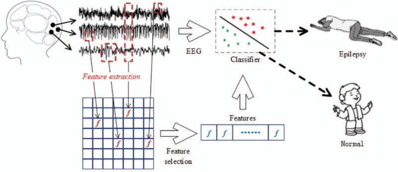
Overall process of EEG signal classification. In feature extraction, GAFDS and extraction methods are used for nonlinear features; a genetic algorithm is used to optimize the selection of the features. The classifiers used for analysis include the k-nearest neighbor, linear discriminant analysis, decision tree, AdaBoost, multilayer perceptron, and Naïve Bayes. EEG = electroencephalogram, GAFDS = genetic algorithm-based frequency-domain feature search.

2.1. Feature extraction

2.1.1. GAFDS method

Genetic algorithm (GA) is a random search method that simulates the biological laws of evolution. GA is a probability optimization method, which exhibits global optimization capability. The following standard parallel GA^[27] is used in this study to search for features in the frequency domain: 

where C is the chromosome coding in GA, E is the individual fitness function, P₀ is the initial population, M is the size of the initial population, Φ is the selection operator, Γ is the crossover operator, Ψ is the mutation operator, and T is the given termination condition.

In signal processing, the frequency domain is a coordinate system that describes the frequency features of the signals. Often used to analyze signal features, a frequency spectrogram reflects the relationship between the frequency and amplitude of a signal. The GAFDS method adopts GA to search for a set of classification-suitable features in the frequency spectrum (Fig. 2).

Figure 2.

Flowchart of genetic algorithm-based frequency-domain feature search.

Figure 3 shows the frequency spectrograms of 5 classes of signals (i.e., A, B, C, D, and E) after fast Fourier transformation (FFT). The x-axis represents the frequency, whereas the y-axis represents the amplitude. A significant variation occurs in each class at a certain frequency, such as the amplitudes enclosed in red boxes. By contrast, the amplitudes enclosed in green boxes are difficult to distinguish. The proposed feature extraction method searches for several superior frequency spaces in the frequency spectrogram. Subsequently, the mean values of the amplitudes in the spaces are used as the features. Then, the GA with global search capability is employed to search for the optimal frequency spaces.

Figure 3.

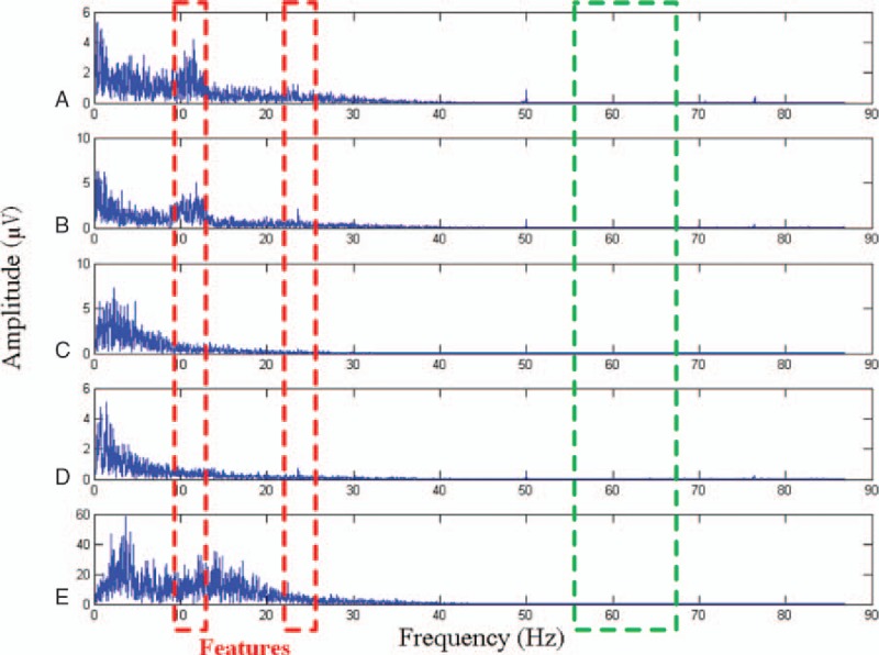
Frequency-domain feature extraction. The features in the red boxes are suitable for classification, whereas those enclosed in green boxes are ineffective. The goal of the genetic algorithm-based frequency-domain feature search method is to find a number of effective features.

A time series X{x₁, x₂, …, x_n} with a length of n is formed after a signal is sampled. Then, a series Y{y₁, y₂, …, y_m} with a length of m is obtained by applying FFT to X. For i, j ∊ [1, …, m] and i < j, 

The f_ij in Eq. (2) is the feature in the frequency interval [i, j].

The main process of using GA in frequency intervals involves obtaining several frequency features with high distinguishing capabilities. Details of this process follow.

• 1.Individual encoding

  On the assumption that the total number of features to be searched for is α, the length of the individual coding array C is 2α. The value of each element in C is between 0 and the highest frequency. Both C_2i and C_2i + 1 (0 ≤ i < α) from C are taken as the frequency range to calculate the features. As shown in Fig. 4, C₃ and C₄ can be used to calculate the feature f_C3,C4.

  However, the constraint i < j should be applied to calculate feature f_i,j. When i ≥ j, the feature makes no sense. Therefore, a negative slack variable β (when i ≥ j, β = 0) is adopted to implement the constraint.

• 2.Fitness function
  Traversing C to calculate the features yields α features and α slack variables {β₁, β₂, …, β_α}. For the optimization of the features, the samples should ideally present larger interclass distances and smaller intraclass distances in the feature space. LDA is employed to evaluate these features. The calculation involves a large number of iterations; thus, LDA is used because of its high calculation speed. The fitness value is calculated by 

  
• 3.Operators

Figure 4.

Structure of the individual encoding.

In GAFDS, Γ is a multipoint crossover operator, Ψ is a Gaussian mutation operator, and Φ is a roulette wheel selection operator.

2.1.2. Nonlinear features

An EEG signal is random and unstable; thus, using FFT alone cannot effectively distinguish EEG signals. For this reason, other nonlinear methods, namely, sample entropy, Hurst exponent, Lyapunov exponent, and multifractal detrended fluctuation analysis (MFDFA), are used in this study to extract the effective features.

Proposed by Richman and Moorman^[28] in 2000, sample entropy, which improves on Pincus approximate entropy,^[29] is a measure of regularity to quantify the levels of complexity of a time series. Sample entropy is often used to extract the features of EEG signals.^[5,6] A feature based on sample entropy is defined by 

Sample entropy requires 3 parameters: signal length, sn; embedding dimension, sm; and similar tolerance, sr. The value of sr is the standard deviation of X multiplied by parameter χ.

The Hurst exponent was first proposed by England hydrologist H.E. Hurst.^[30] Often used in the chaos–fractal analysis of a time series, it is an index for judging whether the time series data are random walk or biased random walk. In a previous study,^[7] the Hurst exponent was adopted as the main feature for EEG classification and defined by 

The Lyapunov exponent is used for computing how fast nearby trajectories in a dynamic system diverge. This exponent is one of the features used to recognize chaotic motions.^[31] In this study, the largest Lyapunov exponent is used as a feature of EEG and given by 

In physiology, fractal structures exist in physiological signals. Multifractals can reveal the complexity and inhomogeneity of fractals. MFDFA is the algorithm used for analyzing the multifractal spectrum of a biomedical time series.^[32]

Figure 5 shows the MFDFA-based multifractal spectra of the 5 classes of signals (i.e., A, B, C, D, and E). When the q-order moments of the wave function are −8, −6, −4, −2, 0, 2, 4, 6, and 8, several multifractal spectra are formed. Three points from each multifractal spectrum, namely, p₁, p₂, and p₃, are selected, where p₁ is the point with the minimum h_q, p₂ with the maximum h_q, and p₃ with the maximum D_q. Each point has 2 coordinate values; thus, 6 features are obtained. The 6 features include 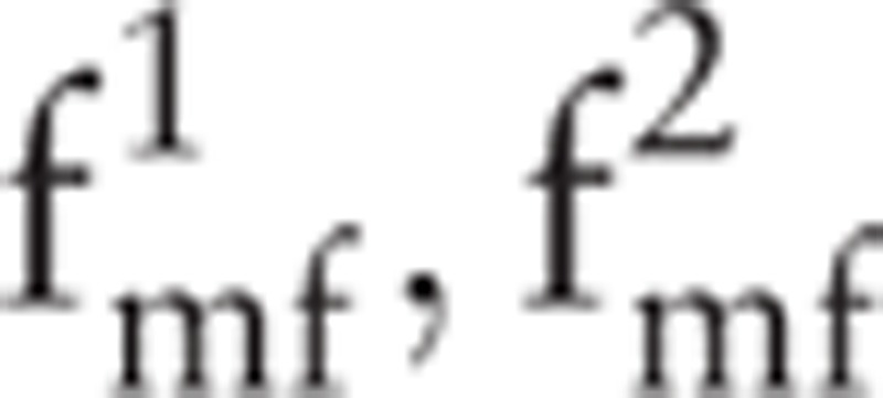(i.e., the h_q and D_q values of p₁); 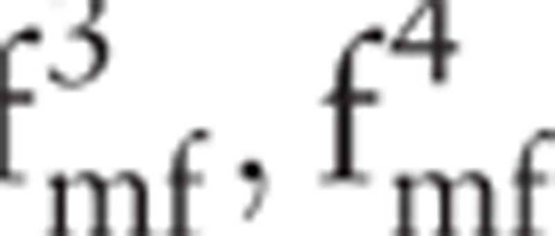(i.e., the h_q and D_q values of p₂); and 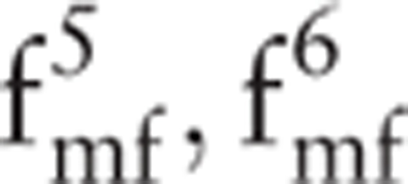(i.e., the h_q and D_q values of p₃). The maximum value of D_q is always equal to 1; accordingly, 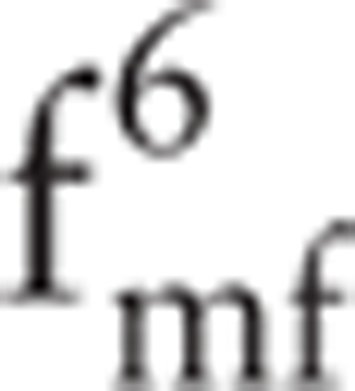can be removed. Finally, the feature set can be obtained using MFDFA. At the same time, the detrended fluctuation analysis value of the signal is also a feature: 

Figure 5.

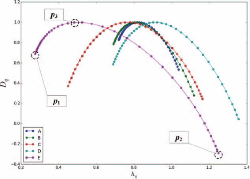
Multifractal detrended fluctuation analysis-based multifractal spectra of the 5 classes of signals. For each sample, the coordinates of p₁, p₂, and p₃ in the fractal spectrum are taken as the features of the sample.

2.1.3. Feature selection and optimization

Feature extraction is useful in data visualization and comprehension. It reduces the requirement for data calculation and storage as well as the time for training and application. Numerous signal feature extraction algorithms are used in practice. Researchers often combine several feature extraction algorithms to analyze data. However, the use of multiple algorithms usually results in feature dimension expansion and feature redundancy. Feature selection reduces the dimension of a feature space and thus facilitates data training and application.

The selection of an optimal feature subset is an nondeterministic polynomial time problem; therefore, GA is used to search for the optimal feature subset. The algorithm codes individuals in the population in a binary array whose length is the number of features. In the array, 1 means the feature is selected, whereas 0 indicates otherwise. The object function of the algorithm is 

where FPR is the fall-out or false positive rate and TPR is the sensitivity or true positive rate.

2.2. Classification model

After feature extraction, multiple models, including k-NN, LDA, decision tree (DT), AdaBoost (AB), MLP, and NB, are used to classify EEG signals.

Cover and Hart^[33] first proposed k-NN. The main idea of k-NN is as follows: if most of the k samples most similar (nearest in feature space) to a sample belong to a class, then the sample also belongs to that class.

LDA was introduced into pattern recognition and artificial intelligence by Belhumeur et al.^[34] The basic functional concept of LDA is projecting high-dimensional pattern onto the optimal discriminant vector space to extract classification information and reduce feature space dimension. After projection, the pattern samples exhibit the maximum interclass distances and the minimum intraclass distances in the new subspace; that is, the pattern presents the best separability in the space.

DT^[35] implements a group of classification rules represented by a tree structure to minimize the loss function on the basis of the known occurrence probability of each situation. This model is a graphical method that intuitively uses probability analysis. The decision nodes resemble branches of a tree, and thus, the model is called a DT.

AB^[36] is an iterative algorithm that trains different classifiers (weak classifiers) with the same training set and combines these weak classifiers of different weights to construct a stronger classifier (strong classifier).

MLP^[37] is a feed-forward ANN consisting of multiple layers of nodes in a directed graph, with each layer fully connected to the next. Each node is a processing element with an activation function. MLP uses backpropagation for training the network to distinguish data.

NB^[38] is the classification method based on Bayes theorem and feature conditional independence assumption. NB originates from classical mathematics and offers solid mathematical basis and stable classification accuracy. In addition, this model only requires few parameters. It is also insensitive to missing data. In theory, the NB model presents minimal error compared with other classification methods.

2.3. Method flow

Figure 6 shows the process of combining the optimization algorithm and classification model. The original dataset is divided into a training dataset and a testing dataset. After feature extraction and selection, a feature subset is acquired from the training dataset. Subsequently, on the basis of the feature subset, features are separately extracted from the training dataset and testing dataset to obtain the new training set and testing set. Finally, a new training set is used to train the classifier and test the classifier on the new testing set.

Figure 6.

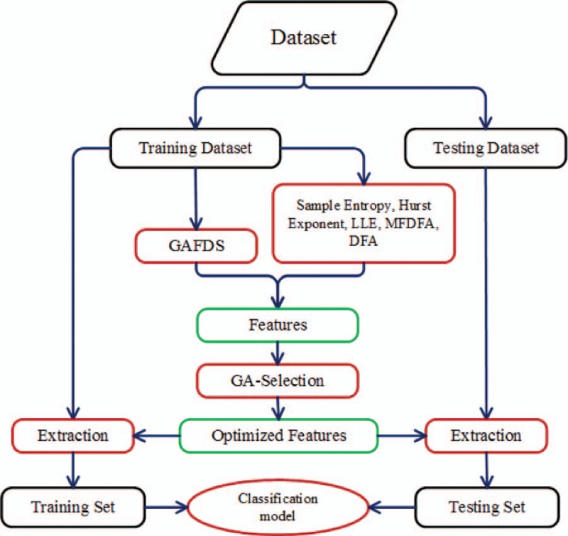
Combination of the optimization algorithm and classification model.

3. Experiments and results

3.1. Dataset

The dataset is obtained from the work of Andrzejak et al.^[39] It includes 5 classes of data (i.e., A, B, C, D, and E). Each class has 100 single-channel EEG samples, each with a length of 23.6 s. The sampling frequency is 173.61 Hz; thus, each sample is a time series with 4097 numbers. Sets A and B are collected when healthy volunteers open and close their eyes. Sets C, D, and E are from epileptics. The samples in set D are recorded from the epileptogenic zone, whereas those in set C are obtained from the hippocampal formation of the opposite hemisphere of the brain. Sets C and D contain only the activities measured during seizure-free intervals, whereas set E only contains seizure activities. The relation among these 5 classes of EEGs is shown in Fig. 7. Numerous previous studies focused on A, E classification; {C, D}, E classification; A, D, E classification; and A, B, C, D, E classification. This paper examines A, E classification; {C, D}, E classification; and A, D, E classification. Figure 8 illustrates the sample data of the 5 classes.

Figure 7.

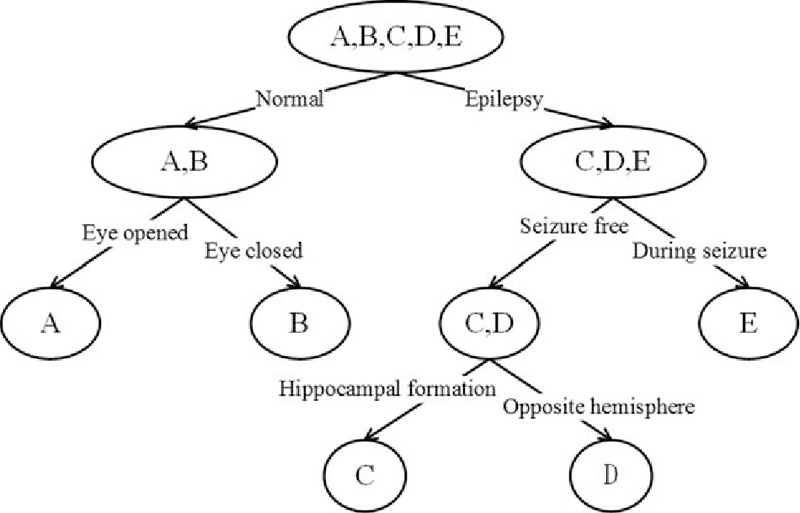
Relation graph of the 5 classes of electroencephalogram signals. A and B are captured from the scalp, whereas C, D, and E come from the intracranial electrodes.

Figure 8.

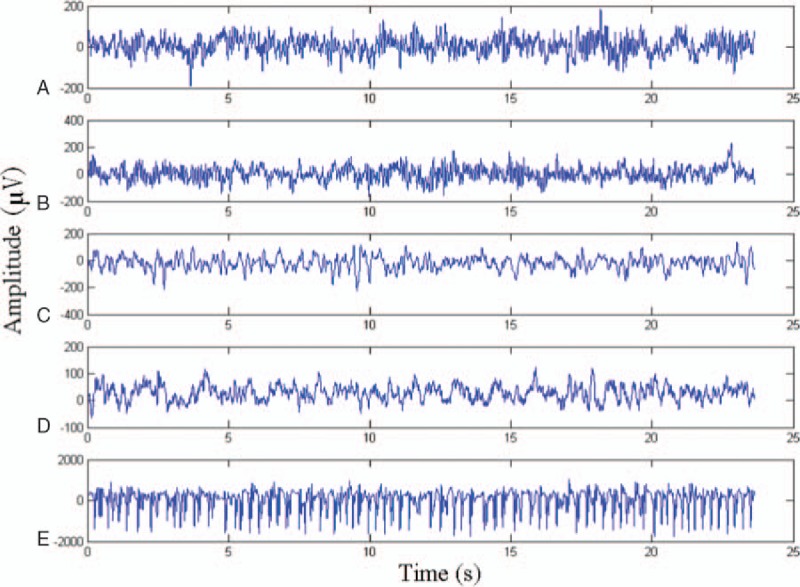
Sample data of the 5 classes (i.e., A, B, C, D, and E).

3.2. Environment and parameter

All the algorithms are written using Python programming language and run on a computer (Ubuntu 14.04 LTS, Core i7-6850K CPU, 3.6 GHz, 128 GB memory space). The algorithms are implemented using Pyevolve^[40] and Scikit-learn^[41] libraries.

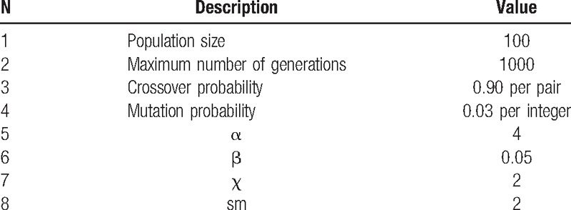
Table 1 lists the parameters used in the experiments. These parameters are based on the general guidelines given in the literature and the authors’ computational experiments on the proposed algorithms.

Table 1.

Parameters and their values.

3.3. Results

3.3.1. Feature extraction and selection

The results of the feature selection inevitably influence the classification results. The nonlinear features of signals do not change across different classification problems. However, the optimization variables of the object function of GAFDS vary across different classification problems, and the selected features are different. In this study, the object function of GAFDS distinguishes the 5 classes. When α = 4, 4 features (i.e., f₁, f₂, f₃, and f₄) are extracted by GAFDS, and 5 features (i.e., f₅, f₆, f₇, f₈, and f₉) are extracted by MFDFA. In addition, sample entropy f₁₀, Hurst exponent f₁₁, largest Lyapunov exponent f₁₂, and DFA feature f₁₃ are obtained.

Figure 9 shows the distributions of the 5 classes of samples in feature space f₁. Most feature values of class A are below 3, whereas most feature values of class E exceed 3. Therefore, classes A and E can be distinguished by feature f_1. Approximately 50% of the samples of classes B and C can be classified by f₁, but the other samples are mixed. Most class C and class D samples are mixed and difficult to distinguish. Overall, classes C and D present outliers, and class E is discrete. Figure 10 shows the distributions of each class in different feature spaces. The median increases from class A to class E for f₄ but decreases for f₆. Feature f₁₃ can effectively distinguish {B, C} and {B, D}. This analysis shows that a single feature usually distinguishes 2 classes at most. Therefore, further analysis of the feature combination is necessary.

Figure 9.

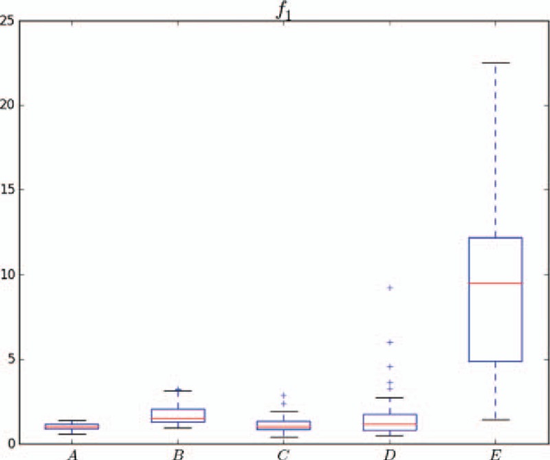
Distributions of the 5 classes of samples in f₁. A and B as well as E and {A, B, C, D} are distinguishable.

Figure 10.

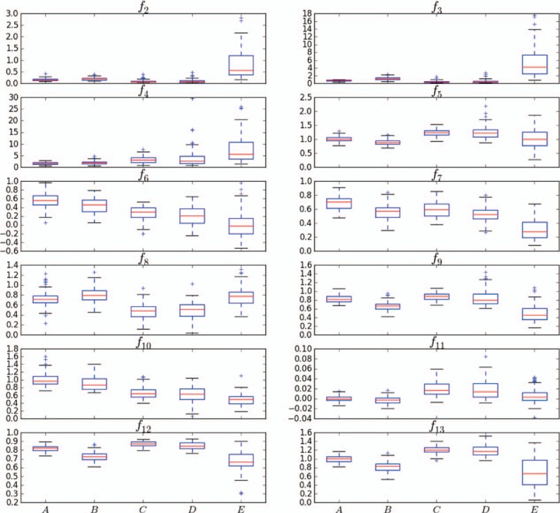
Distributions in feature spaces f₂–f₁₃ of the 5 classes of samples.

As shown in Fig. 11, features f₁, f₄, f₆, f₇, f₉, f₁₀, f₁₁, and f₁₃ are extracted to construct different 2-dimensional feature spaces. A point in the space represents a sample of a class. In space {f₁, f₁₁}, all samples of the 5 classes are concentrated on the left side, and they are difficult to separate. In space {f₄, f₉}, the outlines of classes A, B, E, and {C, D} are clear, but classes C and D are mixed. Every class is discrete in space {f₆, f₇} and {f₁₀, f₁₃}; however, in space {f₁₀, f₁₃}, each class occupies a certain distribution area, and each class crosses only at the edges.

Figure 11.

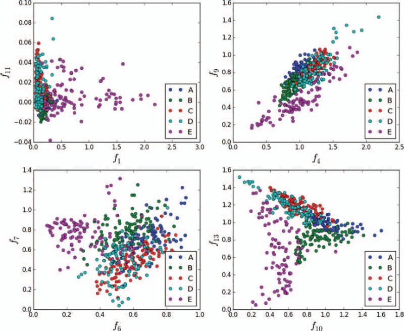
Distributions of the 5 classes in different 2-dimensional feature spaces. In the 2-dimensional combination space (f₁₀, f₁₃), classes E, B, and {A, C, D} are evidently divided into 3 parts.

In 1- or 2-dimensional feature spaces, features can be directly observed. However, as the dimension increases, feature evaluation based on distances is the most direct method, regardless of the classifier. In this study, the features {f₁, f₂, f₃, f₄} extracted by GAFDS are evaluated by comparing the ratios of the interclass distance and intraclass distance of all the classes with those of the nonlinear features {f₁₀, f₁₁, f₁₂, f₁₃}. The interclass distance between 2 classes is their distance in a feature space. With n samples in class A, n feature vectors are generated after feature extraction. Vector represents sample i ∊ A. Accordingly, the intraclass distance of class A is calculated by 

The distance between sample i and itself is 0. The interclass distance between n samples in class A and m samples in class B is calculated by 

Therefore, the ratio of the interclass distance and intraclass distance between class A and class B is 

The ratio of the interclass distance and intraclass distance between a class and itself is 1; that is, r_AA = r_BB = r_CC = r_DD = r_EE = 1.

Table 2 shows the ratios of the interclass distance and intraclass distance of the 5 classes in feature spaces {f₁, f₂, f₃, f₄} and {f₁₀, f₁₁, f₁₂, f₁₃}. The features retrieved by GAFDS are comparable to the nonlinear features.

Table 2.

Ratios of the interclass and intraclass distances of the 5 classes in feature spaces {f₁, f₂, f₃, f₄} and {f₁₀, f₁₁, f₁₂, f₁₃}.

The 5 classes of samples in {f₁, f₂, f₃, f₄} and {f₁₀, f₁₁, f₁₂, f₁₃} feature spaces are simultaneously classified by numerous classical classifiers. The classifiers used, namely, k-NN, LDA, DT, AB, MLP, and NB, are included in the Scikit-learn library. For the k-NN classifier, k = 3. The maximum depth of DT is 5. For the MLP, α = 1. Other parameters use the default values in the library.

A, E classification involves classifying the EEG signals produced by healthy people and epileptics. As shown in Table 3, numerous classifiers can achieve high accuracies by using the listed features.

Table 3.

Classification accuracies of the common classifiers for classes A and E in feature spaces {f₁, f₂, f₃, f₄} and {f₁₀, f₁₁, f₁₂, f₁₃} (using k-fold cross-validation, k = 5).

The classification of {C, D} and E means classifying EEG signals produced during seizure-free intervals and during seizure. GA is used to select the features for this classification. The results are shown in Table 4. A, D, E classification is the classification of EEG signals acquired from healthy people, seizure-free epileptics, and epileptics during seizure. The results are shown in Table 5.

Table 4.

Classification accuracies of common classifiers for {C, D} and E classes in feature spaces {f₁, f₂, f₄, f₅, f₇, f₈, f₉, f₁₀, f₁₂} (using k-fold cross-validation, k = 5).

Table 5.

Classification accuracies of the common classifiers for A, D, E in feature spaces {f₁, f₂, f₄, f₅, f₆, f₉, f₁₀, f₁₁, f₁₂, f₁₃} (using k-fold cross-validation, k = 5).

3.3.2. Classification results

In the previous section, the features extracted by GAFDS are optimized for the classification problems of the 5 classes. However, for real binary or 3-classification problems, the optimization object should be set according to the requirement; that is, the object function in Eq. (3) should be adjusted.

Table 3 shows good results for A, E classification. For the {C, D} and E classification problem, Table 6 lists the results based on the features extracted by GAFDS, whereas Table 7 illustrates the results based on the features optimized by GA selection from the GAFDS-obtained features and other features.

Table 6.

Accuracies for {C, D} and E classification based on the features extracted by GAFDS.

Table 7.

Accuracies for {C, D} and E classification based on the features optimized by GA selection.

For a multiclassification problem, Tables 8 and 9 show that GAFDS and the feature selection method can obtain good results for A, D, E classification.

Table 8.

Accuracies for A, D, E classification based on features extracted by GAFDS.

Table 9.

Accuracies for A, D, E classification based on the features optimized by GA selection.

4. Discussion

4.1. GAFDS method

EEG signals are nonlinear, time varying, and unbalanced. FFT is a global linear method. However, a frequency spectrum does not reflect the frequency changes in the time domain; thus, FFT has certain limitations when applied to nonstationary signal analysis. As shown in Table 2, the features extracted by GAFDS present poor cohesiveness compared with other features. For example, class E presents a wide distribution in f₆, whereas class D has numerous outliers. Thus, features {f₁, f₂, f₃, f₄} in Figs. 9 and 10 are standardized to obtain new features {} within the range [0, 1]. After feature standardization, the accuracy of the AB classifier presents minimal reduction, whereas those of other classifiers remain unchanged, as shown in Table 10. These results indicate that the features extracted by GAFDS have better independence.

Table 10.

Table 2 presents a comparison based on Eq. (11) between the features extracted by GAFDS with nonlinear features. As shown in the table, r_BA is good even though the features extracted by GAFDS present poor cohesiveness. Therefore, the features extracted by GAFDS are superior to the nonlinear features in A, E classification. Furthermore, GAFDS presents great extensibility. GAFDS selects features by searching a frequency spectrum; however, it can also search for new features in a Hilbert spectrum and several other signal spectra. Figure 12 shows the instantaneous frequency change in the samples in classes A and E in the time domain after Hilbert transformation. A period along the time axis can also be searched using GAFDS. Subsequently, the average value of the positive instantaneous frequencies in this period can be used as a feature. With this feature, the accuracy of the LDA classifier can reach up to 74.5% when classifying samples in classes A and E.

Figure 12.

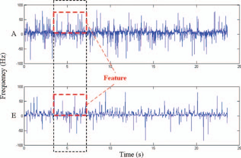
Instantaneous frequencies of the samples in classes A and E whose mean value t in the red box is taken as the feature of the sample.

4.2. Analysis and comparison of classification results

As shown in Tables 3–5, the classifiers have different accuracies in different feature spaces. This study uses few features and small searching space. The classification results show that the GA-based feature selection can obtain superior feature combination.

For the A, E classification problem, the features extracted by GAFDS can effectively facilitate classification. For the {C, D} and E classification, Tables 6 and 7 show that the classification accuracy increases after combining new features with the features extracted by GAFDS and feature selection. However, when the complexity of the problem increases, such as in the A, D, E classification (Tables 8 and 9), the classification accuracies of the classifiers using the features extracted by GA selection are not significantly higher than those of the classifiers using the features only generated by GAFDS. Furthermore, the AB classifier performs well in the 2-classification problem but poorly in the multiclassification problem because the parameters of the classifiers are not optimized.

Table 11 shows a comparison of the classification results between recent classifiers and the classification scheme proposed in this paper. Using wavelet transform-based statistical features, largest Lyapunov exponent, and approximate entropy features, Murugavel et al^[21] developed an ANN and hierarchical multiclass SVM with a new kernel classifier to improve the accuracy for A, D, E classification to 96%. Sharma and Pachori^[46] used the features based on 2- and 3-dimensional phase space representation of intrinsic mode functions as well as an SVM classifier to classify {C, D}, E. Their work achieved a classification accuracy of 98.67%. The scheme proposed in the present study exhibits better classification results with the use of several classifiers based on the GAFDS-selected features and nonlinear features.

Table 11.

Comparison of the results of existing models for EEG classification and the scheme proposed in this paper.

5. Conclusion

EEG provides important information for epilepsy detection. Feature extraction, selection, and optimization methods exert significant influence in EEG classification. In this study, a GA-based frequency feature search method is proposed for EEG classification. The method presents global searching capability to search for classification-suitable features in EEG frequency spectra and combine these features with nonlinear features. Finally, GA is used to select effective features from the feature combination to classify EEG signals.

The experimental results show that the standardization and normalization of the features extracted by GAFDS do not affect the accuracy of the classification results and thus indicate that the features extracted by GAFDS have good independence. Compared with nonlinear features, GAFDS-based features allow for high classification accuracy. Furthermore, GAFDS can effectively extract features of instantaneous frequency in the signal after Hilbert transformation; thus, GAFDS presents good extensibility.

For the A, E and {C, D}, E 2-classification problems and the A, D, E 3-classification problem, the GAFDS-based features and optimized features are used by several classifiers (i.e., k-NN, LDA, DT, AB, MLP, and NB). The classification accuracies achieved are better than those by previous classification models.

In our future work, we will use GAFDS to extract new features and use time-domain, frequency-domain, or time–frequency domain features in feature optimization and selection to achieve improved classification accuracy. The parameters and performance of GAFDS also need further improvement. The precision, complexity, and dimension of EEG data increase; thus, we need to continuously improve the extraction method and conduct further research on feature selection optimization to meet the challenging requirements of EEG analyses.

References

- [1].Acharya UR, Vinitha Sree S, Swapna G, et al. Automated EEG analysis of epilepsy: a review. Knowledge Based Syst 2013;45:147–65. [Google Scholar]
- [2].Yu PM, Zhu GX, Ding D, et al. Treatment of epilepsy in adults: expert opinion in China. Epilepsy Behav 2011;23:36–40. [DOI] [PubMed] [Google Scholar]
- [3].Altunay S, Telatar Z, Erogul O. Epileptic EEG detection using the linear prediction error energy. Expert Syst Appl 2010;37:5661–5. [Google Scholar]
- [4].Chen L, Zhao E, Wang D, et al. Feature extraction of EEG signals from epilepsy patients based on Gabor Transform and EMD decomposition. Int Conf Nat Comput 2010;3:1243–7. [Google Scholar]
- [5].Zhang A, Chen Y. EEG feature extraction and analysis under drowsy state based on energy and sample entropy. Paper presented at: 2012 5th International Conference on BioMedical Engineering and Informatics; 2012:501–5. [Google Scholar]
- [6].Zhang Y, Ji X, Liu B, et al. Combined feature extraction method for classification of EEG signals. Neural Comput Appl 2016;DOI: 10.1007/s00521-016-2230-y. Epub ahead of print. [Google Scholar]
- [7].Geng S, Zhou W, Yuan Q, et al. EEG non-linear feature extraction using correlation dimension and Hurst exponent. Neurol Res 2013;33:908–12. [DOI] [PubMed] [Google Scholar]
- [8].Ren Y, Wu Y. Convolutional deep belief networks for feature extraction of EEG signal. Int Joint Conf Neural Netw 2014. 2850–3. [Google Scholar]
- [9].Chen L, Zou J, Zhang J. Dynamic feature extraction of epileptic EEG using recurrence quantification analysis. Paper presented at: Proceedings of the 10th World Congress on Intelligent Control and Automation, Beijing; 2012:5019–22. [Google Scholar]
- [10].Tu W, Sun S. Semi-supervised feature extraction with local temporal regularization for EEG classification. Int Joint Conf Neural Netw 2011. 75–80. [Google Scholar]
- [11].Tu W, Sun S. Semi-supervised feature extraction for EEG classification. Pattern Anal Appl 2013;16:213–22. [Google Scholar]
- [12].Rafiuddin N, Uzzaman Khan Y, Farooq O. Feature extraction and classification of EEG for automatic seizure detection. Paper presented at: International Conference on Multimedia, Signal Processing and Communication Technologies, IEEE; 2011:184–187. [Google Scholar]
- [13].Wang D, Miao DQ, Wang RZ. A new method of EEG classification with feature extraction based on wavelet packet decomposition. Tien Tzu Hsueh Pao/Acta Electron Sin 2013;41:193–8. [Google Scholar]
- [14].Lotte F, Congedo M, Lécuyer A, et al. A review of classification algorithms for EEG-based brain-computer interfaces. J Neural Eng 2007;4:R1–3. [DOI] [PubMed] [Google Scholar]
- [15].Li X, Chen X, Yan Y, et al. Classification of EEG signals using a multiple kernel learning support vector machine. Sensors 2014;14:12784–802. [DOI] [PMC free article] [PubMed] [Google Scholar]
- [16].Murugavel ASM, Ramakrishnan S, Maheswari U, Sabetha BS. Combined seizure index with adaptive multi-class SVM for epileptic EEG classification. Paper presented at: International Conference on Emerging Trends in Vlsi, Embedded System, Nano Electronics and Telecommunication System, IEEE; 2013:1–5. [Google Scholar]
- [17].Zou L, Wang X, Shi G, Ma Z. EEG feature extraction and pattern classification based on motor imagery in brain-computer interface. Paper presented at: IEEE International Conference on Cognitive Informatics, IEEE; 2010:536–541. [Google Scholar]
- [18].Djemili R, Bourouba H, Korba MCA. Application of empirical mode decomposition and artificial neural network for the classification of normal and epileptic EEG signals. Biocybern Biomed Eng 2015;36:285–91. [Google Scholar]
- [19].Subasi A, Erçelebi E. Classification of EEG signals using neural network and logistic regression. Comput Methods Prog Biomed 2005;78:87–99. [DOI] [PubMed] [Google Scholar]
- [20].Wang D, Miao D, Xie C. Best basis-based wavelet packet entropy feature extraction and hierarchical EEG classification for epileptic detection. Expert Syst Appl 2011;38:14314–20. [Google Scholar]
- [21].Murugavel ASM, Ramakrishnan S. Hierarchical multi-class SVM with elm kernel for epileptic EEG signal classification. Med Biol Eng Comput 2016;54:149–61. [DOI] [PubMed] [Google Scholar]
- [22].Choi S. Multi-subject EEG classification: Bayesian nonparametrics and multi-task learning. Paper presented at: International Winter Conference on Brain-Computer Interface, IEEE; 2015:1. [Google Scholar]
- [23].Amin HU, Malik AS, Ahmad RF, et al. Feature extraction and classification for EEG signals using wavelet transform and machine learning techniques. Australas Phys Eng Sci Med 2015;38:1–1. [DOI] [PubMed] [Google Scholar]
- [24].Nunes TM, Coelho ALV, Lima CAM, et al. EEG signal classification for epilepsy diagnosis via optimum path forest—a systematic assessment. Neurocomputing 2014;136:103–23. [Google Scholar]
- [25].Satapathy SK, Dehuri S, Jagadev AK. ABC optimized RBF network for classification of EEG signal for epileptic seizure identification. Egypt Inform J 2017;18:55–66. [Google Scholar]
- [26].Lin CJ, Hsieh MH. Classification of mental task from EEG data using neural networks based on particle swarm optimization. Neurocomputing 2009;72:1121–30. [Google Scholar]
- [27].Goldberg DE. Genetic Algorithms in Search, Optimization and Machine Learning. Boston, MA: Addison-Wesley Longman Publishing Co., Inc.; 1989. [Google Scholar]
- [28].Richman JS, Moorman JR. Physiological time-series analysis using approximate entropy and sample entropy. AJP Heart Circ Physiol 2000;278:H2039–49. [DOI] [PubMed] [Google Scholar]
- [29].Pincus SM. Approximate entropy as a measure of system complexity. Proc Natl Acad Sci USA 1991;88:2297–301. [DOI] [PMC free article] [PubMed] [Google Scholar]
- [30].Hurst HE. Long term storage capacity of reservoirs. Trans Am Soc Civil Eng 1951;116:776–808. [Google Scholar]
- [31].Wolf A, Swift JB, Swinney HL, et al. Determining Lyapunov exponents from a time series. Phys D Nonlin Phenomena 1985;16:285–317. [Google Scholar]
- [32].Ihlen EA. Introduction to multifractal detrended fluctuation analysis in Matlab. Front Physiol 2012;3:141. [DOI] [PMC free article] [PubMed] [Google Scholar]
- [33].Cover T, Hart P. Nearest neighbor pattern classification. IEEE Trans Inform Theory 1967;13:21–7. [Google Scholar]
- [34].Belhumeur PN, Hespanha JP, Vs KME. Fisherfaces: Recognition Using Class Specific Linear Projection. Computer Vision—ECCV ’96. Berlin: Springer; 1996. [Google Scholar]
- [35].Safavian SR, Landgrebe D. A survey of decision tree classifier methodology. IEEE Trans Syst Man Cybern 1991;21:660–74. [Google Scholar]
- [36].Zhu J, Zou H, Rosset S, et al. Multi-class AdaBoost. Stat Its Interface 2006;2:349–60. [Google Scholar]
- [37].Hassanaitlaasri E, Akhouayri ES, Agliz D, et al. Seismic signal classification using multi-layer perceptron neural network. Int J Comput Appl 2013;79:35–43. [Google Scholar]
- [38].Cheeseman P, Stutz J. Fayyad UM, Piatetsky-Shapiro G, Uthurusamy R. Bayesian classification (AutoClass): theory and results. Advances in knowledge discovery and data mining. Menlo Park, CA: American Association for Artificial Intelligence; 1996. 153–80. [Google Scholar]
- [39].Andrzejak RG, Lehnertz K, Mormann F, et al. Indications of nonlinear deterministic and finite-dimensional structures in time series of brain electrical activity: dependence on recording region and brain state. Phys Rev E 2001;64:116–26. [DOI] [PubMed] [Google Scholar]
- [40].Perone CS. Pyevolve: a python open-source framework for genetic algorithms. ACM SIGEVOlution 2009;4:12–20. [Google Scholar]
- [41].Pedregosa F, Varoquaux G, Gramfort A, et al. Scikit-learn: machine learning in python. J Mach Learn Res 2012;12:2825–30. [Google Scholar]
- [42].Chandaka S, Chatterjee A, Munshi S. Cross-correlation aided support vector machine classifier for classification of EEG signals. Expert Syst Appl 2009;36:1329–36. [Google Scholar]
- [43].Guo L, Rivero D, Dorado J, et al. Automatic epileptic seizure detection in EEGs based on line length feature and artificial neural networks. J Neurosci Methods 2010;191:101–9. [DOI] [PubMed] [Google Scholar]
- [44].Liang SF, Wang HC, Chang WL. Combination of EEG complexity and spectral analysis for epilepsy diagnosis and seizure detection. EURASIP J Adv Signal Process 2010;2010:1–5. [Google Scholar]
- [45].Pachori RB, Patidar S. Epileptic seizure classification in EEG signals using second-order difference plot of intrinsic mode functions. Comput Methods Programs Biomed 2014;113:494–502. [DOI] [PubMed] [Google Scholar]
- [46].Sharma R, Pachori RB. Classification of epileptic seizures in EEG signals based on phase space representation of intrinsic mode functions. Expert Syst Appl 2015;42:1106–17. [Google Scholar]