Clustering: how much bias do we need?

Abstract

Scientific investigations in medicine and beyond increasingly require observations to be described by more features than can be simultaneously visualized. Simply reducing the dimensionality by projections destroys essential relationships in the data. Similarly, traditional clustering algorithms introduce data bias that prevents detection of natural structures expected from generic nonlinear processes. We examine how these problems can best be addressed, where in particular we focus on two recent clustering approaches, Phenograph and Hebbian learning clustering, applied to synthetic and natural data examples. Our results reveal that already for very basic questions, minimizing clustering bias is essential, but that results can benefit further from biased post-processing.

This article is part of the themed issue ‘Mathematical methods in medicine: neuroscience, cardiology and pathology’.

1. Introduction

The perception of the presence—or the absence—of objects by means of the human senses is fundamental to our existence. In everyday life, this task and the reliability with which we are able to perform this task are of utmost importance, e.g. when driving a car. Medical targets of similar relevance are the identification of the presence of malicious tissue in a part of our body, or the identification and quantification of neuro-based behaviourally effective disorders of the human brain, and more.

The great ability of the human mind in mastering perceptional tasks when supported by the eyes has led science and technology to approach such questions mostly via vision. There is a whole branch of modern imaging methods and analyses that, for example, improve the accuracy of localizing brain defects. Imaging procedures are among the best validated methods for, for example, early diagnosis of Alzheimer’s disease, and imaging techniques are used for the efficient therapy of heart diseases, even coupling of diagnostics and therapy. Positron emission tomography, X-ray, computed tomography, magnetic resonance imaging, optical coherence tomography and ultrasound imaging lead a very long list of such methods. In general, these methods are considered just as tools, and the question of what mathematical assumptions and principles underlie these methods is, from the user side, seldom posed.

Recently, the efficacy and helpfulness of the visually based methods, however, seem to approach their limitations. The main reason for this is the increased complexity of the objects that we need or want to deal with, which renders three-dimensional vision insufficient. This becomes apparent in the context of describing, evaluating and comparing different aspects of objects of chemical or biological origin [1–3]. To describe such objects in a most unbiased way forces us to take an extended number of descriptors or markers into account, which leads to a description space the dimension of which greatly exceeds the three dimensions that our visual system generally works in (hearing would offer a much refined approach, but due to the simplicity of visual information, this path has not been followed and to date remains unexplored). In principle, and under favourable circumstances, such high-dimensional complexity can be avoided if the generators of the complexity itself can be accessed. This approach has been followed, for example, in the realm of the dynamics of complex systems, where examples include fractal image compression [4,5], periodic orbit expansion [6–10] and isospectral network reduction [11]. These approaches are strongly based on the existence of simple generative elements of the complexity. Unfortunately, it is generally difficult to detect such generators even if they exist.

One common tool to reduce dimensional complexity are linear and nonlinear projective methods [12]. Often, these are used without rendering account of the fact that these methods are designed to modify the relationships between the objects in the description space. This affects in particular the distance notion underlying clustering (in all of its variants), which provides the basis of the human perception of objects.

(a). How we perceive objects

Seen from the perspective of physics, humans observe the world primarily by measuring forces (within themselves as well as related to the world around). Such measurements depend on several primary given aspects: the properties of the human body itself (most importantly its mass, the time that its existence covers and the nature of physical properties that the body’s sensors provide). Common to all sources of information is that they can never account for the world’s full complexity [13]—a statement that is not accidentally in close vicinity with Gödel’s theorem, or some ideas of Popper [14–16]. Put in different terms, our observation of the world is always accompanied by a reduction of the potentially available information. The destruction of information inherent in this process is the deeper nature of computation (we separate computation from a mere mathematical reformulation of the problem); in a recent model of and proposal of how to measure computation, this has been formalized [13,17]. Clustering is the next step in how we perceive the world, in terms of objects. Conventionally, clustering is defined as the division of a set of usually a large number of items into subsets that express, among themselves and compared to items not in the subset, an increased degree of similarity. This similarity can be expressed and measured in terms of a distance in a space of feature vectors. By attaching the same symbol to all objects within the same subset, clustering provides the basis of cognition, which then is needed as the input for supervised neural network learning. The awareness that we deal with an object of a specific tag type then is at the heart of human object perception.

(b). Feature selection and the curse of dimension

In this way, every model that we have for any aspect of the world is already based on an unavoidable upstream computation. A model can be appropriate or inappropriate, depending on the degree to which the result of this computation proves to be useful to us: the computation must be chosen in accordance with the nature of the object and the purpose of the computation. On an abstract level, this answers our primary question about which clustering algorithm is the best one. The answer depends both on the goal of the clustering, and the nature of the object. This poses the question of which properties to select for achieving optimal clustering. One idea that seemingly circumvents this question is to carry along as many properties as is computationally feasible. While this appears to avoid a bias by feature selection, it leads to high-dimensional spaces in which the clustering then needs to be performed, which not only increases the computational expense.

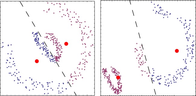
The ‘curse of dimension’ comprises the belief, based on apparent common observational evidence, that clusters appear to rarely persist (or are hard to detect) in sufficiently high-dimensional feature spaces. While on a general level, the verification of such a statement is a difficult task, the statement seems to be guided by the belief that (sub)clusters should generically have the form of Gaussian-like clouds. For such data, with increasing dimension, the distances between feature vectors may tend to identical values, so that the contrast between close and far neighbouring data points, which is at the basis of all clustering, is lost. The assumption of Gaussian data clouds or clusters is closely connected to the idea that the dispersion of the points is mostly due to a random deviation of the data itself or the measuring process around the ‘true’ value. Such an assumption results in an unnecessary bias, in particular, when dealing with complex data, where the data distribution is generally not random, but expresses the process underlying the generation of the data (see below). This Gaussian property assumption underlies one of the most prominent clustering algorithms, and leads in applications to severe problems (figure 1).

Figure 1.

K-means clustering based on a Gaussian-like data distribution assumption is largely unsuccessful for other shapes of data clouds. Only if the two objects move further away from each other can they be considered as Gaussian clouds and be properly separated. Dashed line denotes separating the computed cluster boundaries; filled dots, cluster centres.

In addition to intrinsic or measurement noise, Gaussian-like data distributions can emerge in high dimensions if irrelevant properties are included in the feature vector. Measures that correspond to such properties are then, by standard procedure, rescaled to the whole representation space (e.g. the unit interval), in which they become random variables. It is clear that such features can dominate and fail the next neighbour distance measurement on which clustering is essentially based. To control, monitor and mend such problems, projection methods from higher to lower dimensions are applied. These procedures are extreme steps of computation themselves, and the content of the complexity reduction obtained strongly depends on what aspects vanish upon the applied projection. An illustration of the resulting problems is exhibited in figure 2. A more theoretical instructive example is the projection of the two-dimensional skinny baker map onto a one-dimensional system perpendicular to the expanding direction, which yields a non-trivial Lyapunov spectrum, but an entirely trivial fractal dimension spectrum; only a projection along the expanding direction yields a non-trivial fractal dimension spectrum [18]. While random projections can be used to avoid projection deficits, they corrupt the distance measures that are fundamental for clustering.

Figure 2.

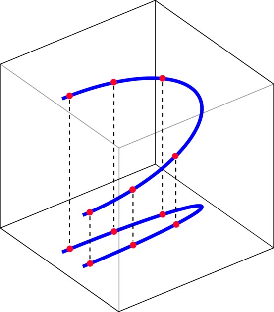
Projections in feature space destroy data distance relations.

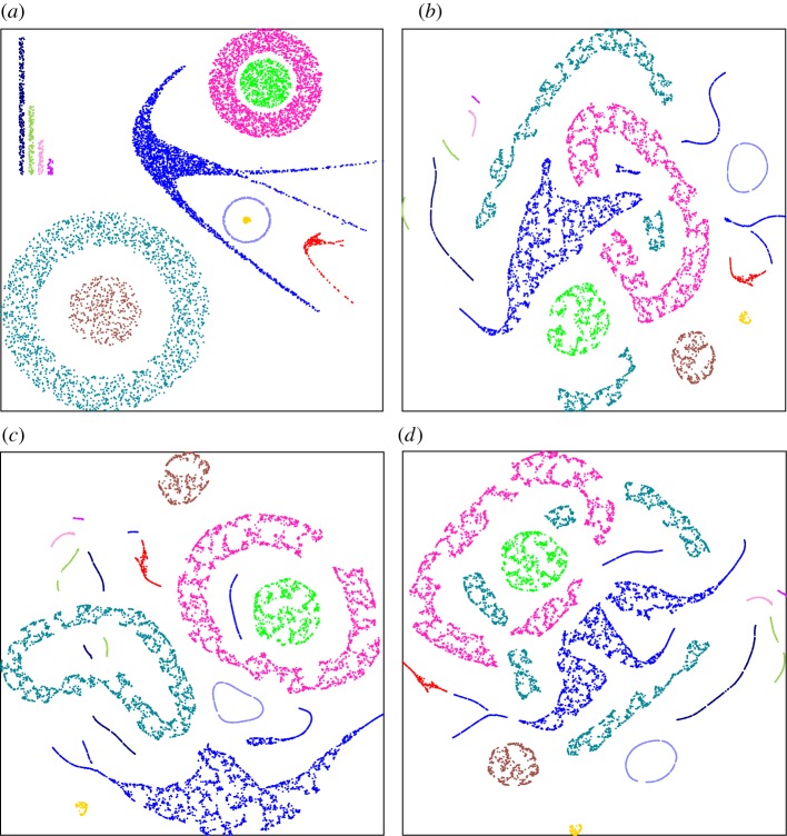
To avoid these difficulties, it has been suggested to follow the data’s local manifold structures and to include a few local dimensions only. Popular algorithms for nonlinear dimensionality reduction are local linear embedding [19], kernel principal component analysis [20–22], ISOMAP [23] and t-SNE [24]. A major problem in doing so is points where manifolds split, such as in the context of shrimp-shaped domains of similar dynamical stability [25]. However, even the most advanced projection methods in use today have great difficulty in providing appropriate projections (figure 3).

Figure 3.

Projection ambiguities of t-SNE. A two-dimensional dataset (a) was first transformed into eight dimensions (see §2) and then projected back into two dimensions using t-SNE ((b–d) three different runs of t-SNE). Point colours are the same in all subfigures. For these parameter settings (perplexity = 30) originally connected clusters may be separated into disconnected subsets. Similar effects are also seen in the presence of noise (see the electronic supplementary material).

(c). Sampling model genericity

The important shape feature that we need to be able to take appropriate care of is the following. From simple reasoning, most elements of a cluster will be the result of the same generating process, obtained via slightly changed parameters of the generative process. Such generative processes lead to distributions that strongly differ from Gaussians [3,26]: whenever two or more parameters are involved in a nonlinear generative process, a shrimp-shaped domain collects the items that have similar properties (figure 4).

Figure 4.

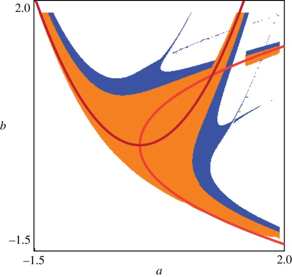
Shrimp-shaped clusters of similar dynamical behaviour (orange, period 1; blue, period 2; white, higher periodic or divergent behaviour) in the (a,b) parameter space of the Hénon map, which is the prototype for all generic properties of nonlinear processes [18]. Two parabolas depict the ‘skeleton’ representing the lowest approximating nonlinearity of the generative nonlinear process [3,25]. K-means, but also the hierarchical Ward-type clustering, cannot properly deal with such shapes.

This example demonstrates that generically, natural objects cluster within convex–concave boundaries. Whereas the property has been shown to hold for maps, it also holds for differential equations, via Poincare sections (upon which the time scale of a system’s behaviour or that related to a feature becomes irrelevant). This is illustrated in figure 5 for the mathematically more involved biochemical reaction differential equation of Decroly & Goldbeter [27], where the emergent dynamics dependent on two of the several parameters are investigated [3].

Figure 5.

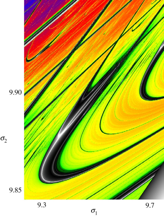
Shrimp-shaped clusters of stable dynamical response of a biochemical model by Decroly & Goldbeter [27], for two selected parameters, σ₁ and σ₂. Stable solutions dwell upon black/white parameter shrimp-shaped domains, where the white lines code for extreme stability of the regular dynamical behaviour and correspond to the parabolas of figure 4. Colours correspond to emergent unstable solution evolution, detected by calculation of the largest Lyapunov exponent [3,18].

Moreover, the shrimp-like shape is inherited into spaces of features. Figure 6 illustrates this on a theoretical level, when the fundamental parameters of the generative process are mapped into several other features resulting in a higher-dimensional feature space. In figure 7, we demonstrate using the purely phenomenological Rulkov model of neuronal spiking [28] that also in feature spaces that are entirely detached from the generative process, shrimp-shaped clusters are abundant.

Figure 6.

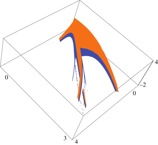
Shrimp in feature space obtained by transforming the data underlying figure 4 according to (other than that it maps parameter into feature space, there is nothing particular about this transformation).

Figure 7.

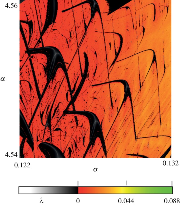
Shrimp domains of a purely phenomenological model of neuronal firing [3,28]. Black denotes domains of stable firing, while red denotes domains of unstable response, expressed in terms of the value of largest Lyapunov exponent λ [18].

This demonstrates that the Gaussian shape assumption is a severe handicap for clustering. Building on the proven relevance of shape bias for clustering, we will address in the next section the question of how the formulation of the search for clusters should be as unbiased as possible.

2. Searching for minimally biased clusters

In the following, we compare and discuss two promising approaches that are fully based on local k-nearest neighbour information and are therefore promising candidates for unbiased clustering: the Phenograph approach (a recently published leading algorithm in the clustering of mass cytometry data with a view to medical application [29]); and a current implementation of our previously described Hebbian learning clustering (HLC) [26,30]. Both algorithms begin by representing data points as nodes of a k-nearest neighbour graph, with distances encoded as graph edge weights. Beyond the graph representation, these algorithms substantially differ. HLC preserves data distance relationships by using an edge weighting that decays with true distance, whereas Phenograph uses the proportion of nearest neighbours shared by the two nodes to define the weight of an edge [29] (Jaccard distance). The clustering procedures themselves are also different. HLC uses the idea of cluster synchronization, modifying edge weights through Hebbian learning [26,30]. Phenograph takes the view that clustering can be achieved by performing community detection as on any other graph, for which a popular and fast, existing algorithm [31] can be used.

For the discovery of unknown relationships in natural data, the most basic requirement for clustering is that it should not impose an a priori bias on the shape of clusters. We scrutinize this aspect using a simple two-dimensional dataset, consisting of two uniform density concentric clusters separated by a thin, low-density ring (figures 8 and 9). The inner disc is a small convex set, while the outer ring is larger, and convex–concave. Any algorithm with reasonable density sensitivity and without an inherent cluster shape bias should be able to essentially separate the inner disc from the outer ring.

Figure 8.

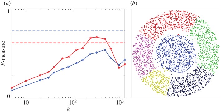
Phenograph performance on two-dimensional data. (a) F-measure (red, unweighted; blue, weighted) as a function of the only algorithm parameter, the number of nearest neighbours k. Dashed lines indicate the F-measure obtained if all points belong to the same cluster. (b) Example clustering result for k=320. Retrieved clusters are distinguished by colours.

Figure 9.

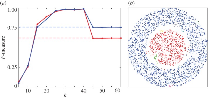
HLC performance on two-dimensional data. (a) F-measure (red, unweighted; blue, weighted) as a function of algorithm parameter, the number of nearest neighbours k. Dashed lines indicate the F-measure obtained if all points belong to the same cluster. (b) Example clustering result for k=40. Retrieved clusters are distinguished by colours. (The weight threshold, as the second parameter of the algorithm, was set to the mean of the final edge weights.)

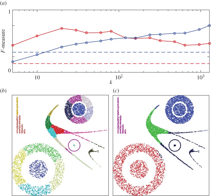
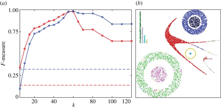
Moreover, a valuable algorithm should also be able to deal with varying data densities, and varying dimensionality. To provide a first, simple challenge, we construct a synthetic dataset in two dimensions composed of test cluster shapes (figures 10 and 11). These data are then transformed into eight dimensions, using the polynomial transformation

2.1

This places the original two-dimensional dataset on a two-dimensional manifold within an eight-dimensional space, and imparts slight density variations within the clusters. While the first two coordinate transformations represent a simple rotation (so that a there exists a projection preserving the original structure), this a priori knowledge will not be available to the algorithms.

Figure 10.

Phenograph performance on higher dimensional data. For display reasons, the clusters obtained in eight dimensions are shown here on the original two-dimensional data. (a) F-measure (red, unweighted; blue, weighted) as a function of the only algorithm parameter, the number of nearest neighbours k. Dashed lines indicate the F-measure obtained if all points belong to the same cluster. (b) Example clustering result for k=80. (c) Example clustering result for k=1280. Retrieved clusters are distinguished by colours.

Figure 11.

HLC performance on higher dimensional data. For display reasons, the clusters obtained in eight dimensions are shown here on the original two-dimensional data. (a) F-measure (red, unweighted; blue, weighted) as a function of algorithm parameter, the number of nearest neighbours k. Dashed lines indicate the F-measure obtained if all points belong to the same cluster. (b) Example clustering result for k=50. Retrieved clusters are distinguished by colours. (A weight threshold value of 0.7 was used.)

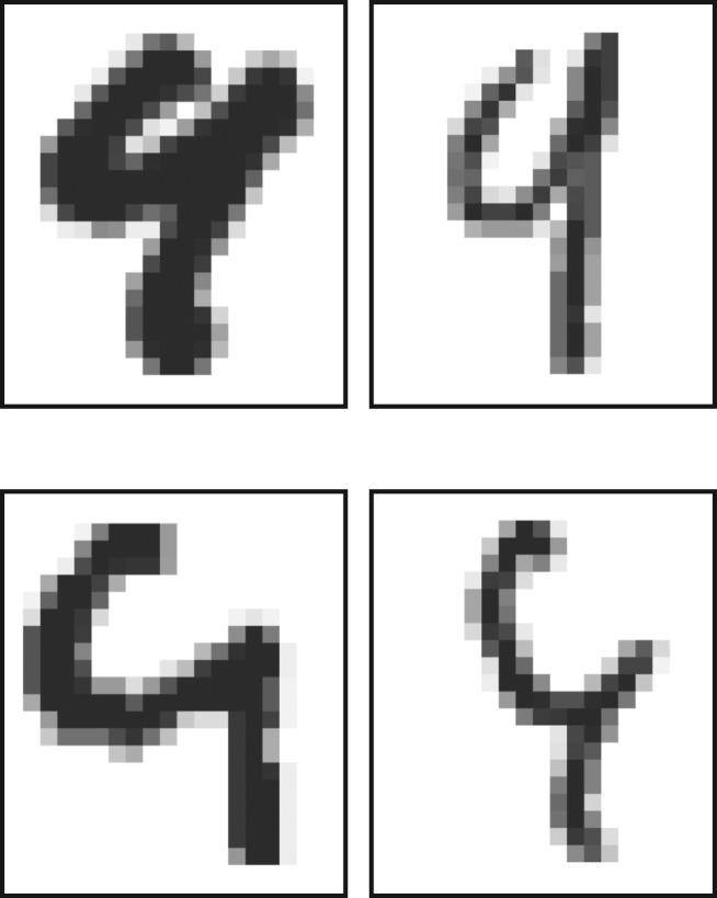
In contrast to the considered synthetic datasets, real-world data are acquired through ‘noisy’ data measurement processes, and can therefore not be expected to display sharp boundaries. In the presence of noise, sets pertaining to different generative processes may even overlap. In such a case, there is no clear way to divide points into their ‘true’ clusters without introducing a model, and thereby introducing a bias. The MNIST dataset of handwritten digits [32] provides an example that is high dimensional, of natural origin and where occasionally two similar generative processes (e.g. the generators of ‘4’ and ‘9’, figure 12), upon parameter variation and enhanced by measurement noise (pixel conversion), generate data clouds that partially overlap. While each person’s handwriting may be self-consistent in that different digits can be easily distinguished, across a population we see a set of data points spreading between the sets of ‘clearly distinguishable’ items. Each MNIST sample has, however, an agreed upon label which suggests this dataset as a reasonable ‘gold standard’ for high-dimensional clustering. We use here a 10 000 digit subset of the MNIST training set, without any additional pre-processing.

Figure 12.

Examples of ‘4’ and ‘9’ digits from the MNIST test dataset [32] that are difficult to classify. Top row: ‘4’. Bottom row: ‘9’.

3. Test results

When dealing with unknown data, it is essential that good clustering results can be achieved over a wide range of algorithm parameters. To assess clustering quality, we use the F-measure [33,34] (also known as F₁ score). This measure is based upon taking the binary harmonic mean between ‘precision’ and ‘recall’ of a given cluster i (the correct labelling) with respect to any retrieved cluster j (the clustering result), i.e.

3.1

where the precision f_p is the proportion of points in the retrieved cluster j that belong to the given cluster i, and the recall f_r is the proportion of points in the given cluster i that have been assigned to the retrieved cluster j. From these measures, the global F-measure is obtained by averaging the maximal F-measures obtained for clusters i, F_i=max_jF_ij, as (unweighted) or (weighted), where n is the number of given clusters i, |i| is the number of points in cluster i, and N is the total number of data points.

We use these statistical measures for the assessment of the clustering algorithms investigated, though it is worth noting that they place algorithms capable of rejecting points as noise, like HLC, at a disadvantage, as the concept of ‘no label’ is not inherent in the F-measure, unless such points are explicitly excluded (see below).

(a). Artificial data

(i). Two dimensions

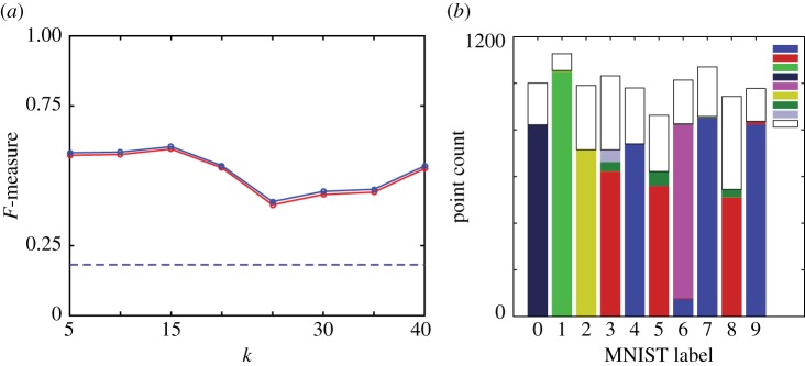
Surprisingly, Phenograph does not solve our simple two-dimensional clustering task in a satisfactory manner (figure 8). Over a very wide range of its only parameter (the number of nearest neighbours k), we find that Phenograph fails to connect the outer ring of the dataset into a single cluster. Moreover, long before the outer ring becomes connected, the inner disc begins to join the outer ring. Why such an algorithm, apparently based on local information, might exhibit this behaviour will be discussed in detail in §3b. The same dataset, however, can be easily clustered by HLC (figure 9), with stable results over a wide parameter range.

(ii). Higher dimensions

Returning to our eight-dimensional dataset (cf. equation (2.1)), we find the same performance issue of Phenograph. In figure 10, we observe a tendency for Phenograph to divide the clusters into sections. For large k, more global artificial boundaries are inserted. Similar effects are seen also in the presence of noise (see the electronic supplementary material). HLC is able to successfully cluster these data, for a reasonable range of k (figure 11).

(b). Natural data

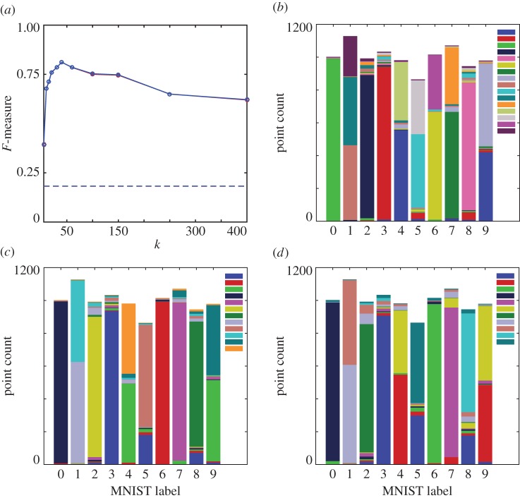
The 784 dimensional MNIST subset poses a substantial challenge for both Phenograph (figure 13) and HLC (figure 14). The F-measure for Phenograph shows a defined peak of around 0.8 for k=40; HLC shows a generally lower F-measure across the tested parameter range and is seemingly outperformed by Phenograph. Looking closer at individual Phenograph clustering results, we see that across almost an order of magnitude of its parameter k, it partitions many of the digits into two or three large sections. The sizes of these partitions grow with increasing k; for very large k they span across different digits. Around k=40, where the highest F-measure is located, some of the partitions are almost the same size as the true clusters. The individual clustering results for HLC are of a fundamentally different nature. Although most clustering algorithms show a tendency to assign points to major clusters, HLC does not have this property [26,30]. HLC generates many clusters also of small size that in an interpretive step can be discarded as noise. For the calculation of the F-measure, this does not favour HLC. The majority of its misclassified data is due to the merging of data labelled as {3,5,8} and {4,7,9}, respectively, where this same cluster merging pattern has been observed in the t-SNE representation of MNIST digits [24], and is consistent with some of the common misclassifications of digits on the MNIST test dataset (e.g. figure 12). This misclassification might be caused by ‘data bridges’ that in human perception are abolished.

Figure 13.

Phenograph, MNIST data (10 000 digits from the MNIST ‘training set’). (a) Unweighted (red) and weighted (blue) F-measure as a function of parameter k. Dashed lines indicate F-measures for case where all points assigned to the same cluster. Clustering results for (b) k=20, (c) k=40, (d) k=150. Results shown as stacked bars where colours depict the different clusters to which each digit has been assigned by the clustering (original classes ‘0’ to ‘9’ do not contain an identical number of elements). Inset in (b)–(d) shows distinct cluster colour labels.

Figure 14.

HLC, MNIST data (10 000 digits from the MNIST ‘training set’). (a) Unweighted (red) and weighted (blue) F-measure as a function of parameter k. Dashed lines indicate F-measures for case where all points assigned to the same cluster. (b) Clustering result for k=15. Result shown as stacked bars where colours depict the different clusters to which each digit has been assigned by the clustering (original classes ‘0’–‘9’ do not contain an identical number of elements). Inset in (b) shows cluster colour labels used; white corresponds to points assigned to clusters of size less than 50. (The weight threshold was set to the mean of the final edge weights.)

4. Discussion

(a). Importance of data ‘bridges’

To scrutinize the data bridges that we suspect to be the origin of the observed merging of digits {3,5,8} and {4,7,9}, we add after the HLC algorithm a controllable interpretive step. Consider the situation depicted in figure 15, where the edges connected to data points in the bridges are characterized by an increased betweenness centrality, compared to edges in the bulk. Pruning the highest betweenness centrality edges from the graph may therefore separate the centres (figure 15). This basic idea is also used in some community detection algorithms [35].

Figure 15.

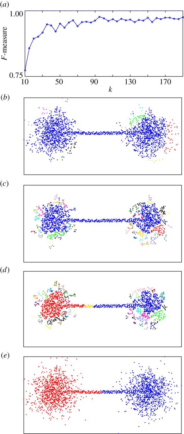
Effect of betweenness centrality pruning on a single ‘dumbbell’ shaped cluster. (a) HLC clustering result F-measure versus k for example dataset in (b)–(d). (b) HLC clustering result for k=50. (c) HLC clustering result for k=10. (d) HLC clustering result for k=10 after betweenness centrality pruning of top 2% of edges. (e) Phenograph clustering result (k=1000).

For the MNIST dataset, this procedure breaks down most of the grouped clusters into the desired sets. Primarily only the {4,9} cluster remains connected (figure 16). However, in the process, numerous points have been moved into very small clusters, which makes it difficult to quantify the quality of the obtained clustering using an F-measure.

Figure 16.

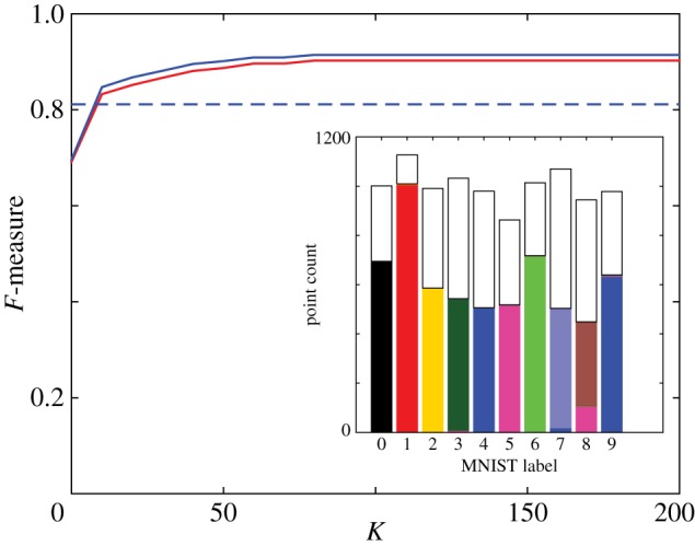
Effect of disregarding small clusters. MNIST dataset as a function of the cluster size K below which clusters are disregarded. HLC (k=15, edges with highest betweenness centrality have been discarded): solid lines (unweighted, red; weighted, blue). Phenograph (k=40): dashed lines (unweighted, red; weighted, blue). Inset: HLC clustering (k=15) after betweenness centrality clipping, with clusters smaller than K=80 displayed white.

To compensate for this effect, we re-calculate the F-measure after disregarding points assigned to clusters below a minimum size K. (This is similar to the effect of disregarding points with no clear label, e.g. [29].) By following this approach, we see that the F-measure of the betweenness centrality pruned HLC result rises sharply as a function of K, saturating at K=80 (figure 16). The best Phenograph result contains only larger clusters, so discarding such small clusters has no effect (figure 16). Using HLC, a cleaner and more complete separation may be possible following this approach, but this is not our focus here.

We have seen that the two apparently closely related algorithms considered here give completely different outcomes on our test datasets. The behaviour of HLC and how this can be exploited for clustering has been elucidated in the previous section and elsewhere [26,30]. In the following, we would like to contribute an analysis of the behaviour of Phenograph.

(b). Understanding community-based clustering

We believe the cluster splitting behaviour we observed from Phenograph when applied to our nearly constant density synthetic data may arise from the community detection algorithm underlying Phenograph. The particular algorithm used by Phenograph, from [31], searches for the partition of the graph that maximizes modularity. Graph modularity Q [35] measures the trade-off between intracluster connections and intercluster connections with respect to a partitioning of the nodes into clusters, and can be written as [31]

4.1

where A_ij is the (weighted) adjacency matrix of the graph, , , c_i is the label assigned to point i, and δ(c_i,c_j)=1 if c_i=c_j, and 0 otherwise. Maximizing the modularity on a k-nearest neighbours graph, however, can have unexpected consequences, when the spatial extent of the clusters exceeds the range of the k-nearest neighbour connections.

Consider, for illustration, a one-dimensional dataset of uniform density, containing L points. Intuition suggests that all L points should be assigned to the same cluster. Suppose instead that the set of points were to be broken up into equally sized clusters of size c, and that the k-nearest neighbour graph is unweighted. Under these assumptions, we can evaluate the modularity as a function of cluster size c. Within each cluster C, for even k, we have

4.2

where

4.3

corrects for the edges outside each cluster. Noting that 2m=Lk, and that there are approximately L/c clusters, this gives

4.4

where

4.5

is a correction for the two clusters at the ends of the set, 1≤c≤L and 1≤k<L−1. Keeping L and k fixed, Q is a function of c with a maximum at c<L (figure 17). Thus, even in this very simple case, maximizing modularity leads to an artificial partitioning of the set. This observation is independent of the method used to maximize Q. As a consequence, any community detection algorithm based on modularity maximization can be expected to show a similar effect.

Figure 17.

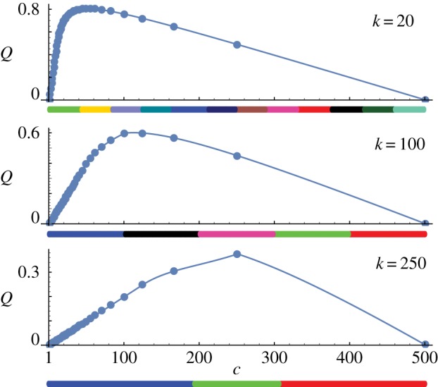
Maximizing modularity on a one-dimensional set. Plots of Q(c) according to our approximation, for L=500, k as indicated. Filled circles indicate Q(c) at points L/j, j∈{1,…,500}, rounded down to the nearest integer. Below the c-axis of each plot is an example Phenograph clustering result for the same value of k, with colours denoting different clusters.

The assumption of unweighted edges should lead to an overestimate (i.e. a conservative estimate) of the value of c maximizing Q. This is because any spatial weighting scheme for clustering will assign lower weights to longer edges. Simulations with Phenograph of a line of 500 equally spaced points reveal cluster sizes consistent with our prediction of the value of c, until the equal cluster size assumption breaks down at large k (figure 17). In more than one dimension for clusters of uniform density, a similar situation may occur. In high dimensions, for clusters with a single dominant density peak, this may not be a problem, but for extended clusters with low-density contrast some caution may be needed.

5. Outlook and conclusion

The focus of this paper has been on where bias enters clustering analysis, and how to deal with it. Our thesis is that bias must be well understood, and be appropriately and carefully controlled, at every step of the data analysis. Even before starting a clustering procedure, the most relevant and informative features must be selected. This selection naturally introduces bias, that must be consistent with the question to be addressed. A poor selection of features cannot be compensated by nonlinear transformations or clustering algorithms. Selection of irrelevant features, in addition, can destroy our ability to detect data structures. In our synthetic data examples, which contain only ‘relevant’ information, appropriate feature selection has been sidestepped. Instead, these examples demonstrate the importance of keeping bias to the lowest reasonable level in the clustering step. As clustering is a strong computation that destroys information, only careful application of algorithms with minimal bias towards cluster form can provide a rich data canvas on which further interpretation can be performed. We see this deferral of delicate interpretive decisions as a service that clustering algorithms should offer. In HLC, for example, the cluster graph structure can be preserved, permitting graph theoretical tools to be applied, to incorporate specific extra information, biasing the outcome towards the kind of ‘true’ clustering result that we are looking for. The specific example using betweenness centrality on the MNIST training digits given above was only provided for illustration purposes. In general, a bias must be carefully chosen that permits the desired question to be answered on the one hand, and on the other hand is general enough to be reliably applicable beyond the specific example on which it is calibrated. On that basis, the discrimination of ‘noise’ by HLC (that might seem at first view to speak against our minimal clustering bias view) can be seen as follows: extracting the major data features in a first step provides a useful structural skeleton in feature space, to which minor and more subtle data features can be related. This could be achieved, for example, by a sequential clustering approach, or a distance-based label reassignment; decisions that would, of course, be specific to the objects of interest in the data.

Requiring that generally applicable clustering algorithms should directly answer specific questions of high-dimensional natural data may be simply asking too much. Questions such as, ‘what are the different cell types present in these data?’ are difficult to separate from the bias imposed by historical developments of the field. By minimizing clustering bias, new viewpoints on old assumptions may become accessible, opening the door to gaining novel insight potentially beyond, and in contrast to, commonly used data categories.

Data accessibility

The proprietary synthetic datasets used in this paper are included in the electronic supplementary material.

Authors' contributions

All authors designed the research, performed the research, generated the figures, and wrote and approved the manuscript.

Competing interests

The authors declare no competing interests.

Funding

The authors are supported by the Swiss National Science Foundation (grant nos. 200021_153542/1 and CR32I3 159660).

References

- 1.Schuffenhauer A, Zimmermann J, Stoop R, van der Vyver JJ, Lecchini S, Jacoby E. 2002. An ontology for pharmaceutical ligands and its application for in silico screening and library design. J. Chem. Inf. Comput. Sci. 42, 947–955. ( 10.1021/ci010385k) [DOI] [PubMed] [Google Scholar]
- 2.Ott T, Kern A, Schuffenhauer A, Popov M, Acklin P, Jacoby E, Stoop R. 2004. Sequential superparamagnetic clustering for unbiased classification of high-dimensional chemical data. J. Chem. Inf. Comput. Sci. 44, 1358–1364. ( 10.1021/ci049905c) [DOI] [PubMed] [Google Scholar]
- 3.Gomez F, Stoop RL, Stoop R. 2014. Universal dynamical features preclude standard clustering in a large class of biochemical data. Bioinformatics 30, 2486–2493. ( 10.1093/bioinformatics/btu332) [DOI] [PubMed] [Google Scholar]
- 4.Barnsley MF. 1988. Fractals everywhere. Boston, MA: Academic Press Professional. [Google Scholar]
- 5.Jacquin A. 1989. Fractal theory of iterated Markov operators with applications to digital image coding. Atlanta, GA: Georgia Tech Theses and Dissertations.
- 6.Cvitanovic P. 1988. Invariant measurement of strange sets in terms of cycles. Phys. Rev. Lett. 61, 2729–2732. ( 10.1103/PhysRevLett.61.2729) [DOI] [PubMed] [Google Scholar]
- 7.Stoop R, Parisi J. 1991. On the convergence of the thermodynamic averages in dissipative dynamical systems. Phys. Lett. A 161, 67–70. ( 10.1016/0375-9601(91)90546-K) [DOI] [Google Scholar]
- 8.Stoop R, Parisi J. 1992. On the influence of the grammar on the entropy spectrum of dissipative dynamical systems. Physica D 58, 325–328. ( 10.1016/0167-2789(92)90120-C) [DOI] [Google Scholar]
- 9.Stoop R, Joller J. 2011. Mesocopic comparison of complex networks based on periodic orbits. Chaos 21, 016112 ( 10.1063/1.3553643) [DOI] [PubMed] [Google Scholar]
- 10.Stoop R, Arthur BI. 2008. Periodic orbit analysis demonstrates genetic constraints, variability, and switching in Drosophila courtship behavior. Chaos 18, 023123 ( 10.1063/1.2918912) [DOI] [PubMed] [Google Scholar]
- 11.Bunimovich LAB, Webb B. 2014. Isospectral transformations—a new approach to analyzing multidimensional systems and networks. Springer Monographs in Mathematics New York, NY: Springer. [Google Scholar]
- 12.Alanis-Lobato G, Cannistraci CV, Eriksson A, Manica A, Ravasi T. 2015. Highlighting nonlinear patterns in population genetics datasets. Sci. Rep. 5, 8140 ( 10.1038/srep08140) [DOI] [PMC free article] [PubMed] [Google Scholar]
- 13.Stoop R, Stoop N, Bunimovich L. 2004. Complexity of dynamics as variability of predictability. J. Stat. Phys. 114, 1127–1137. ( 10.1023/B:JOSS.0000012519.93677.15) [DOI] [Google Scholar]
- 14.Gödel K. 1931. Über formal unentscheidbare Sätze der Principia Mathematica und verwandter Systeme I. Monatsh. Math. Phys. 38, 173–198. ( 10.1007/BF01700692) [DOI] [Google Scholar]
- 15.Gödel K. 1931. Diskussion zur Grundlegung der Mathematik. Erkenntnis 2, 135–151. ( 10.1007/BF02028146) [DOI] [Google Scholar]
- 16.Popper K. 1935. Logik der Forschung. Vienna, Austria: Springer. [Google Scholar]
- 17.Stoop R, Stoop N. 2004. Natural computation measured as a reduction of complexity. Chaos 14, 675 ( 10.1063/1.1778051) [DOI] [PubMed] [Google Scholar]
- 18.Peinke J, Parisi J, Rössler OE, Stoop R. 1992. Encounter with chaos: self-organized hierarchical complexity in semiconductor experiments. Berlin, Germany: Springer. [Google Scholar]
- 19.Roweis ST, Saul LK. 2000. Nonlinear dimensionality reduction by locally linear embedding. Science 290, 2323–2326. ( 10.1126/science.290.5500.2323) [DOI] [PubMed] [Google Scholar]
- 20.Jolliffe IT. 2002. Principal component analysis. Springer Series in Statistics Berlin, Germany: Springer. [Google Scholar]
- 21.Schölkopf B, Smola A, Müller KR. 1998. Nonlinear component analysis as a kernel eigenvalue problem. Neural Comput. 10, 1299–1319. ( 10.1162/089976698300017467) [DOI] [Google Scholar]
- 22.Shawe-Taylor JS, Cristianini N. 2004. Kernel methods for pattern analysis. New York, NY: Cambridge University Press. [Google Scholar]
- 23.De Silva V, Tenenbaum JB. 2003. Global versus local methods in nonlinear dimension reduction. Adv. Neural Inf. Process. Syst. 15, 721–728. [Google Scholar]
- 24.Van der Maaten L, Hinton G. 2008. Visualizing data using t-SNE. J. Mach. Learn. Res. 9, 2579–2605. [Google Scholar]
- 25.Stoop R, Benner P, Uwate Y. 2010. Real-world existence and origins of global shrimp organization on spirals. Phys. Rev. Lett. 105, 074102 ( 10.1103/PhysRevLett.105.074102) [DOI] [PubMed] [Google Scholar]
- 26.Stoop R, Kanders K, Lorimer T, Held J, Albert C. 2016. Big data naturally rescaled. Chaos Solitons Fract. 90, 81–90. ( 10.1016/j.chaos.2016.02.035) [DOI] [Google Scholar]
- 27.Decroly O, Goldbeter A. 1982. Birhythmicity, chaos, and other patterns of temporal selforganization in a multiply regulated biochemical system. Proc. Natl Acad. Sci. USA 79, 6917–6921. ( 10.1073/pnas.79.22.6917) [DOI] [PMC free article] [PubMed] [Google Scholar]
- 28.Rulkov NF. 2002. Modeling of spiking-bursting neural behavior using two-dimensional map. Phys. Rev. E 65, 041922 ( 10.1103/PhysRevE.65.041922) [DOI] [PubMed] [Google Scholar]
- 29.Levine JH. et al 2015. Data-driven phenotypic dissection of AML reveals progenitor-like cells that correlate with prognosis. Cell 162, 184–197. ( 10.1016/j.cell.2015.05.047) [DOI] [PMC free article] [PubMed] [Google Scholar]
- 30.Landis F, Ott T, Stoop R. 2010. Hebbian self-organizing integrate-and-fire networks for data clustering. Neural Comput. 22, 273–288. ( 10.1162/neco.2009.12-08-926) [DOI] [PubMed] [Google Scholar]
- 31.Blondel VD, Guillaume JL, Lambiotte R, Lefebvre E. 2008. Fast unfolding of communities in large networks. J. Stat. Mech. 2008, P10008 ( 10.1088/1742-5468/2008/10/P10008) [DOI] [Google Scholar]
- 32.Lecun Y, Bottou L, Bengio Y, Haffner P. 1998. Gradient-based learning applied to document recognition. Proc. IEEE 86, 2278–2324. ( 10.1109/5.726791) [DOI] [Google Scholar]
- 33.Aghaeepour N, Finak G, The FlowCAP Consortium, The DREAM Consortium, Hoos H, Mosmann TR, Brinkman R, Gottardo R, Scheuermann RH. 2013 Critical assessment of automated flow cytometry data analysis techniques. Nat. Methods 10, 228–138. ( 10.1038/nmeth.2365) [DOI] [PMC free article] [PubMed] [Google Scholar]
- 34.Weber LM, Robinson MD. 2016. Comparison of clustering methods for high-dimensional single-cell flow and mass cytometry data. Cytometry A 89, 1084–1096. ( 10.1002/cyto.a.23030) [DOI] [PubMed] [Google Scholar]
- 35.Newman MEJ, Girvan M. 2004. Finding and evaluating community structure in networks. Phys. Rev. E 69, 026113 ( 10.1103/PhysRevE.69.026113) [DOI] [PubMed] [Google Scholar]
Associated Data
This section collects any data citations, data availability statements, or supplementary materials included in this article.
Supplementary Materials
Data Availability Statement