

Abstract
Spreading depolarizations are implicated in a diverse set of neurologic diseases. They are unusual forms of nervous system activity in that they propagate very slowly and approximately concentrically, apparently not respecting the anatomic, synaptic, functional, or vascular architecture of the brain. However, there is evidence that spreading depolarizations are not truly concentric, isotropic, or homogeneous, either in space or in time. Here we present evidence from KCl-induced spreading depolarizations, in mouse and rat, in vivo and in vitro, showing the great variability that these depolarizations can exhibit. This variability can help inform the mechanistic understanding of spreading depolarizations, and it has implications for their phenomenology in neurologic disease.
Keywords: Spreading depolarization, cortical spreading depression, susceptibility, velocity, anisotropy
Introduction
Spreading depolarizations (SD) are massive disruptions of ionic, metabolic, and vascular homeostasis that propagate slowly and approximately concentrically across the gray matter of the brain.1–4 Once considered a curiosity, SD are now recognized as contributing to neurologic diseases as diverse as migraine,5–7 stroke,8 subarachnoid hemorrhage, and traumatic brain injury.2,4
Given their clinical significance, much still remains unclear about SD. Though to a first approximation they are uniform, disregarding synaptic, cytoarchitectural, and vascular architecture, this characterization does not bear up under scrutiny. With the possible exception of retina,9 SD are not completely concentric or isotropic; however this deviation from concentricity has not been well characterized. SD also have apparent cytoarchitectonic preferences. Leão10–12 and later others13–15 showed that SD were unlikely to propagate into retrosplenial cortex. There is also an apparent tropism of SD for superficial or dendritic layers, rather than deeper layers of cortex.16–18 The mechanisms of these tropisms are unclear, but myelin content, astrocytic density, and vascular disruption have all been advanced as explanations.19,20 Finally, it is well known but under-reported that SD vary considerably over time.14
The spatial and temporal heterogeneity of SD are important, because the factors that influence and constrain SD have the potential to explain basic features of the phenomena, which in turn could lend insight into clinical approaches. Thus we systematically examined the characteristics of SD in different preparations that would allow us to assess their heterogeneity. We show that SD susceptibility as well as propagation varies by cortical location, and by depth within the cortex. We show that non-uniform propagation is the rule, not the exception, for SD, and that this anisotropic propagation becomes more prominent with time, likely due to different relative refractory periods. Finally, we report patterns of SD propagation that suggest both vascular and cytoarchitectonic modulation, and suggest avenues for future research.
Methods
All experiments were performed in accordance with the National Research Council Guide for the Care and Use of Laboratory Animals.21 Analysis and reporting were performed according to the ARRIVE criteria.22 All experiments were approved by the Institutional Animal Care and Use Committees of the University of Utah and the University of California Los Angeles.
SD preparation
Male C57Bl/6J mice (n = 33) or Sprague-Dawley rats (n = 14), 3–6 months of age, were used to avoid the known effects of sex on SD susceptibility.23,24 Animals were anesthetized with isoflurane (5% induction, 1.4–1.7% maintenance) and mounted on a stereotaxic frame (Kopf Instruments, Tujunga, CA, USA). Vital signs (oxygen saturation, heart rate, respiratory rate, body temperature) were monitored and stabilized using a physiological monitoring apparatus (MouseStat, Kent Scientific, Torrington, CT, USA). In mice, the parietal skull was exposed between bregma and lambda, and a standardized region measuring 3.2 mm × 2.4 mm centered between bregma, lambda, sagittal sinus, and temporal ridge was thinned to transparency. A burr hole for SD induction was created in one of four different locations (one location per animal; coordinates represent distance from bregma): Lateral – 2.6 mm posterior and 4.2 mm lateral. Medial – 2.6 mm posterior, 0.5 mm lateral. Anterior – 0.5 mm posterior and 2.3 mm lateral. Posterior – 4.6 mm posterior, 2.3 mm lateral. A second burr hole for local field potential recording was created 4.6 mm posterior and 0.4 mm lateral to bregma in all animals, for electrophysiologic confirmation of SD. In rats, either a craniotomy with boundaries 1 mm from bregma, lambda, sagittal sinus, and temporal ridge was made (n = 5), or, for depth electrode recordings (n = 9), a large (1–2 mm diameter) burr hole was made (2 mm lateral, 4 mm posterior to bregma). For the craniotomy preparation, SD was induced midway between bregma and lambda at the temporal ridge (corresponding to the Lateral location in mice); for the depth electrode preparation, a second burr hole (2 mm lateral, 7 mm posterior to bregma) was used.
Optical imaging
Briefly,25,26 the cortex was illuminated by a white-light LED (5500 K, Phillips Lumileds, San Jose, CA, USA) and reflected light (optical intrinsic signal; OIS) was collected with a lens system consisting of two f/0.95 lenses connected front to front focused on a high-sensitivity 8-bit charge-coupled device camera (Mightex CCE-B013-U, Pleasanton, CA, USA). Images were acquired at 2 Hz for the duration of the experiment. In all experiments, SD was induced by continuous application of 1 M KCl solution for 1 h. Excess KCl was removed by the capillary action of rolled filter paper placed adjacent to the KCl burr hole. Thin but intact skull preparation restricted KCl exposure and SD induction to the burr hole (all SDs were seen emanating from the burr hole).
Optical spectroscopy
A fiber optic probe (R400-7-UV/VIS, Ocean Optics; Dunedin, FL, USA) (225 µm diameter) was placed 3.9 mm posterior and 1.4 mm lateral to bregma, parfocal with the OIS camera, and used to collect reflected light for spectroscopy. A spectrometer (USB400-UV-VIS, Ocean Optics) collected probe output at 1 Hz with a 1 s integration time and 5 nm boxcar smoothing. Hemoglobin saturation was derived using the Beer-Lambert law as previously described.26
Electrophysiology
In all mice and rat craniotomy experiments, local field potential was recorded with ACSF-filled (in mM: 125 NaCl, 3 KCl, 1.25 NaH2 PO4, 2 CaCl2, 1 MgCl2, 25 NaHCO3, 10 glucose) glass microelectrodes (3 MΩ) advanced 500 µm into the LFP burr hole.27 The ground electrode was placed in the cervical muscles. Local field potentials were recorded using an Axopatch 1D amplifier (Molecular Devices, Sunnyvale, CA, USA) (0–500 Hz band pass; digitized at 1 kHz) synchronized with imaging data by a LabView Virtual Instrument (National Instruments, Austin, TX, USA). In rat depth electrode experiments (n = 9), a two- or three-electrode array (ACSF-filled, 10 µm diameter tips, 10 MΩ resistance, horizontal separation 200–400 µm, vertical separation 100–1800 µm) was advanced into the burr hole. Interelectrode distances were verified after each recording and confirmed with histology. A reference electrode (Ag/AgCl) was inserted subcutaneously in the neck. Electrical signals were collected at a DC-10 kHz bandwidth, amplified with an ISODAM-8A bioamplifier (WPI Inc, Sarasota, FL, USA) digitized at 200 Hz (Micro1401, A-M Systems, Sequim, WA, USA), and stored for off-line analysis using Spike2 software (CED Co., Cambridge, UK).
Brain slice recordings
Briefly,28 male C57Bl/6 mice (n = 83 slices, 37 animals, age 1–3 months) were deeply anaesthetized with isoflurane and decapitated. Coronal slices of 400 µm thickness were cut in an ice-cold oxygenated sucrose solution using a vibratome (MA752 Motorised Advance Vibroslice, Campden Instruments, Loughborough, UK). The slices were then incubated in an oxygenated ACSF solution at room temperature for at least 1 hour before the experiments. SD was induced using a custom microfluidic device with ejection and suction ports that allowed precise focal ejection. SD was induced by substituting K+ for Na+ in the ACSF in defined steps, until threshold was reached.28,29
Data analysis
Optical intrinsic signal (OIS) analysis
In each experiment, the field of view (480 × 480 pixels) was divided into three rectangular regions of interest (ROIs, 480 × 180 pixels) placed perpendicular to the advancing SD wave front. A plot representing the change in cortical reflectance over time was generated for each ROI. SD were identified as a propagating change in reflected light during optical imaging. A histogram representing pixel brightness distribution was generated for each ROI. Any ROI which showed saturated pixels was discarded from further analysis. “Full” SD were defined as SDs that propagated across the whole imaging field. “Partial” SD did not propagate across the whole imaging field, and had variable patterns of propagation as described below. The SD perfusion response was measured as shown in Figure 1(d), between the maximum and minimum in wave-associated reflectance, and then normalized by dividing each SD amplitude by the average amplitude of all SDs in all experiments. Amplitude, duration, and velocity were only measured for full SDs.
Figure 1.

Susceptibility and hemodynamic characteristics of SD vary by induction site. (a) Schematic shows SD induction sites (black circles) superimposed over the mouse brain with labeled cytoarchitecture. Induction sites: medial: retrosplenial cortex; lateral: auditory cortex; anterior: forepaw somatosensory cortex; posterior: primary visual cortex. Rectangle shows boundaries of thin skull region; white circle shows location of spectroscopy probe. (b) Box whisker plots show total, full, and partial SD counts originating from the four induction sites, measured from an equal-sized region of interest to allow comparisons between the four locations. There is a significant difference in total, full and partial SD, driven by large differences in the posterior (visual cortex) induction site (ANOVA followed by a Tukey multiple comparison test, *p < 0.05, **p < 0.01, ***p < 0.001, n(animals) = 9, 8, 9, 7, for the medial, lateral, anterior and posterior sites respectively). (c) Inter-event intervals for medial, lateral, posterior, and anterior induction sites. (ANOVA followed by a Tukey multiple comparison test, *p < 0.05, **p < 0.01, ***p < 0.001, n = 9, 7, 9, 7, for the medial, lateral, anterior, and posterior sites respectively). (d) Left trace shows equal and opposite changes in total hemoglobin (HbT) and optical intrinsic signal (OIS) during SD, showing that OIS can be used to infer blood volume changes. Right trace shows typical SD OIS profile. Amplitude of hemodynamic changes was measured from peak (hypoperfusion) to trough (hyperperfusion) of SD-associated reflectance change. Left graph. Normalized change in perfusion between the different induction sites. (Data were normalized by dividing the change in perfusion for each induction site by the average change in perfusion for all sites). The posterior induction site had a higher normalized change in perfusion compared to the other induction sites. Right graph. Duration of perfusion between the different induction sites. The posterior site had a significantly reduced duration compared to the anterior and medial sites but not the lateral site. The lateral induction site had a significantly decreased duration of perfusion compared to the medial induction site (ANOVA followed by a Tukey multiple comparison test, *p < 0.05, **p < 0.01, ***p < 0.001, n = 6, 5, 7, and 4 for the medial, lateral anterior and posterior sites respectively). (e) Schematic shows typical hemoglobin saturation trace during multiple SDs. Hemoglobin desaturation amplitude (left graph) and half width (right graph). Hemoglobin desaturation was significantly smaller in posterior compared to anterior and lateral induction sites, despite being the closest site to the spectroscopy probe. No difference between the different induction sites was seen in half width duration (ANOVA followed by a Tukey multiple comparison test, *p < 0.05, ***p < 0.001, n = 4, 8, 4, 5, for the medial, lateral, anterior and posterior sites respectively).
Wavefront tracings and wavespeed maps
We segmented the moving wavefront of the CSD waves using a variant of the regularized front segmentation method presented in Chang et al. 2012,51 modified by the shape prior renormalization scheme of Chang et al. 2014.52 In order to improve the signal to noise ratio, we used bilinear interpolation to downsize the original 644 × 480 movies to 322 × 240. In the frame-by-frame differences of these movies, the region immediately upwind of the CSD wavefront is brighter than the surrounding regions. We segmented these bright regions as they grew using the aforementioned methods, approximating the running wave speed on a coarser 161×120 lattice. Wherever we were not able to obtain good segmentations, either due to low signal to noise or partial fronts, we manually traced the wavefront by hand. With the front tracings available, the wave speed map was computed by inverting the eikonal equation. We performed this inversion by interpolating using bicubic interpolation and computing the gradient by central differencing. The regularized segmentation method was completed in Fiji ImageJ (2.0.0-rc-44). The eikonal equation inversion was performed in Python 2.7 using Scipy 14.0’s interpolate.interp2d method. The source code for our wavefront tracing method can be found at https://github.com/joshchang/BrennanLab.
Statistics
All analysis was performed using GraphPad Prism v5.03. A p < 0.05 was considered significant. Data were plotted as box-whisker plots showing median, 25th percentile, 75th percentile, and minimal and maximal values. Comparisons between the different induction sites were made using one-way ANOVA followed by a Tukey multiple comparison test, or a Student’s t-test. Comparisons between different ROIs were performed with repeated measure ANOVA followed by Dunnet’s test.
Results
Incidence of SD varies by location of induction
We examined the characteristics of SD induced by identical technique (1 hour continuous 1 M KCl administration) from four locations at opposite ends of a standardized 3.2 × 2.4 mm region of thinned skull that was centered between bregma, lambda, sagittal suture, and temporal ridge. The four stimulus locations were each in different cytoarchitectonic regions: the medial stimulation site was in retrosplenial granular cortex, just medial to the medial edge of parietal association cortex (in mm from bregma: 2.6 posterior, 0.5 lateral); the lateral site was in auditory cortex, just lateral to the posterolateral edge of barrel cortex (2.6 posterior, 4.2 lateral), the anterior stimulation site was in forelimb somatosensory cortex (0.5 posterior, 2.3 lateral), and the posterior site was in primary visual cortex (4.6 posterior, 2.3 lateral) (Figure 1(a)).
There was a significant difference in number of total SD elicited per hour over the four groups (one-way ANOVA F-25.75, p < 0.001, n = 9, 8, 12, 8 for the medial, lateral, anterior and posterior locations, respectively). This result was driven by significant differences between the posterior induction site and all other induction sites (p < 0.001) (Figure 1(b)).
The spatial extent of SD also varied significantly by location. The posterior site, with the highest number of induced SD, also had the highest number of partial SD – waves that did not propagate through the whole imaging field. In contrast, the anterior induction site had significantly fewer SDs than the posterior (p < 0.001 for total SDs), but also had a significantly lower number of partial SDs (Figure 1(b)) because most anterior SDs were full (i.e. propagated through the entire imaging field).
Because the imaging field (and the underlying cortex) was longer in the anteroposterior than the mediolateral axis, we compared the number of SDs that reached a fixed, identical distance (470 pixels, or 2.3 mm) from the site of induction, in order to make the comparison meaningful across all four locations. However, because anterior and posterior inductions both propagated along the long axis of the cortex, we were also able to compare them along the whole length of the window. Here again significant differences were observed between the two locations, with significantly greater numbers of total, full, and partial SDs for posterior vs. anterior inductions (Student’s t-test, p < 0.001 for total, p < 0.05 for full, and p < 0.001 for partial SDs, respectively).
With the difference in incidence of SDs came differences in the timing of events. The posterior induction site had the shortest and most consistent (least variable) inter-event interval (ANOVA followed by Tukey test, p < 0.05 for medial and p < 0.001 for lateral and anterior sites), while the anterior site had the longest and most variable inter-event interval. Medial and lateral locations were intermediate in value (Figure 1(c)).
SD hemodynamic characteristics vary by cortical location
Optical intrinsic signal (OIS) imaging is used to measure hemodynamic changes, and is primarily driven in vivo by hemoglobin concentration and/or saturation in each voxel30 (light scatter changes, other absorbers, and intrinsic fluorescence also contribute31,32). We used spectroscopy to verify that reflectance in our wavelength range corresponded to changes in total hemoglobin rather than changes in saturation (Figure 1(d)). We then were able to characterize increases and decreases in reflectance as relative decreases and increases in blood volume, respectively. In order to evaluate the hemodynamic changes associated with SD independently of large baseline fluctuations, we chose the distance between the maximum (hypoperfusion peak) and minimum (hyperperfusion peak)3,25 of SD-associated reflectance as our metric of SD-associated hemodynamic amplitude change. We used the time between these peaks as a proxy for SD duration. We used a 160 × 480 pixel region of interest, placed 160 pixels distant from each location, to compare the responses of each.
There were significant differences in amplitude and duration of SD perfusion correlates, with the posterior induction site showing both the highest amplitude (p < 0.01) and the shortest duration of blood volume change (p < 0.001 for medial and p < 0.05 for anterior; ANOVA with post hoc Tukey test) (Figure 1(d)).
SD involves changes in hemoglobin saturation as well as blood volume.3,26,33 We used a spectroscopic probe to measure hemoglobin saturation from a fixed region of interest in the posteromedial portion of the imaging window (Figure 1(a)). Because of its fixed location, this region of interest was at different distances from each induction site (in mm from induction sites: posterior 1.1, medial 1.6, lateral 3.1, anterior 3.5), thus we hypothesized that hemoglobin desaturations would likely decrease with distance and thus might not reveal differences between locations. Surprisingly however, the posterior induction site, despite being closest to the spectroscopic probe, revealed significantly smaller desaturations than lateral and anterior SD (p < 0.001 for lateral and anterior respectively), which were more distant (Figure 1(e)).
Significant differences between first and subsequent SDs for all locations
A consistent finding in all locations tested was that the first SD was significantly different from all following waves. This was most prominent for SD velocity, which was dramatically different between the first and subsequent events. It was also more variable, with a much wider distribution of velocities (Figure 2(a)). No significant differences in SD velocity were found between locations. For hemodynamic correlates, there was a significant decrease in the amplitude of SD blood volume change, though there was no difference in duration (Figure 2(b)). Another dramatic difference between first and subsequent SD was the extent of SD propagation – we observed no first SD that did not propagate through the entire imaging field, whereas subsequent SD could be either full or partial (examples in Figure 5).
Figure 2.
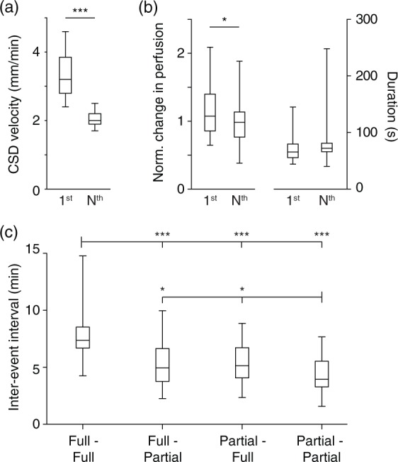
Velocity and hemodynamic amplitude are larger for first vs. subsequent SD. (a) SD velocity, though not significantly different between cortical induction sites (data not shown), shows significant decreases (as well as decreases in variability) when comparing first to all subsequent SD. (b) Left graph: Amplitude of SD-associated blood volume change is larger in first compared to subsequent SD. Right graph: There was no significant difference in duration of blood volume changes (*** p < 0.001, *p < 0.05, Student’s t-test, n = 20 mice). (c) Inter-event intervals from all four induction sites divided into four types of transitions: full to full, full to partial, partial to full, partial to partial. Full–full transitions had the longest intervals; partial–partial the shortest, with intermediate values for full–partial and partial–full transitions (*p < 0.05, **p < 0.01, ***p < 0.001, Tukey multiple comparison test, n = 91, 79, 74, and 28 for the “full–full,” “full–partial,” “partial–full,” and “partial–partial” groups, respectively).
Figure 5.
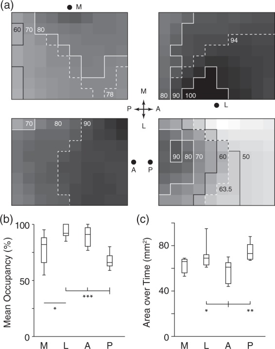
Cumulative SD propagation characteristics. (a) Panels summarize all experiments for each induction location. Each panel is an 8 × 10 grid rendering of the imaged region. Each square shows percentage occupancy by SD over all experiments for that induction location. For example, a square showing 50% occupancy was occupied by 50% of all SD waves induced. Dashed contour shows median occupancy value, giving a measure of central tendency. Each induction location has very different occupancy patterns. Also note that for all but posterior induction, there is a relative avoidance of the posteromedial (top left) squares, corresponding to retrosplenial cortex. (b) Mean percent occupancy for the four induction sites. Lowest percent occupancy was for the posterior site (primary visual cortex), highest was for lateral site (auditory cortex), corresponding with the highest and lowest proportion of partial SD, respectively. (c) Cumulative area exposed to SD over all experiments. Despite the large number of partial events, the high number of SD induced from the posterior site led to the largest area exposed.
Pattern of propagation is inhomogeneous in all locations, and varies between locations
SD induced from all four locations deviated significantly from concentric propagation, and the pattern of propagation was distinct for each location and each experiment, both initially and over time. While the first SD tended to be the most concentric and isotropic, even these usually contained inhomogeneities in both the shape of the wave front and in the rate of propagation across the imaging field (Figures 3 and 4).
Figure 3.

SD propagation patterns for all experiments. Each square represents a SD propagation pattern. Total number of incidences is given above each pattern. Patterns without a number occurred less than 5 times.
Figure 4.

Heterogeneous SD patterns. All contours are plotted at 4-s intervals. All scale bars are 1 mm. (a) All 8 SD from a medial induction experiment. Last panel is superimposed over a standard deviation map of the experiment, which shows veins as dark, arteries as bright (because they change shape during SD) and cortex as intermediate gray. SD propagation varies considerably between each event. Note that first SD propagates significantly faster than all subsequent events (also seen in (b), (d), and (f)). (b) Alternating full and partial SD in a posterior induction experiment. Possible modulation of wave shape by cortical vein (first, third, and fourth panels; also see (c), second and third panels of (d) and (g)). (c) Eccentric propagation that avoids prior locations, avoids retrosplenial cortex (see also (d)). (d) Increasing avoidance of retrosplenial cortex. Possible vascular modulation of wavefront. (e) Partial SD followed by spiral SD that circles the location of prior partial (see also (c)). (f) Heterogeneous SD propagation in rat. (g) Varying propagation rate, possibly modulated by midline vein. Map at right plots derived SD velocity over each pixel, highlighting heterogeneity (methods in Chang et al.51,52).
Subsequent SD tended to become more irregular in shape, as well as slower in velocity and smaller in spatial extent. Examples included bi-lobed waves, double waves, and spiral waves, as well as waves that propagated across only part of the imaged field. There was also evidence of re-entrant waves, which left the imaging field only to return from another location (Figures 3 and 4). In a subset of OIS experiments performed in rat (lateral induction only; n = 5), we confirmed these observations: propagation was inhomogeneous even for first SD, and became more inhomogeneous and slower over time (Figure 4(f)).
In order to systematize the analysis of wave patterns, we divided the imaging field into an 8 × 10 grid of equally sized squares and quantified the incidence of each square on the grid experiencing a SD passage, for all SD elicited from a given location. For example, if a square was affected by every SD elicited, its incidence was 100%. This gave a summary view of SD susceptibility (formally, SD occupancy) for each location. There were significant differences in the overall propagation pattern from each location (Figure 5(a)). Other summary measures were the total area occupied by SD, and the mean percent activation of all regions, for each stimulus location. The former gives an index of how much cortex is affected by SD over time; the latter reveals how likely a given SD was to affect the whole cortex. Despite having the lowest percent activation score due to the large number of partial events, posterior-induced SD occupied the largest area over time, by virtue of the very high frequency of events. Conversely, anterior-induced SD occupied the smallest area over time due to a small total number of events, but had a very high activation score due to the low proportion of partial events (Figure 5(b) and (c)).
Factors modulating SD propagation
Modulation of SD by prior SD: refractory phenomena
The most obvious effect of prior SD on subsequent events was the decrement seen after the first SD (see above). However, prior events continued to have major effects on subsequent SDs over time. A prominent phenotype was an increased likelihood of partial SD with increasing numbers of SD events (correlation of all partial SD with all total SD, Pearson’s r 0.78, p = 3e-8, n = 342). When observing the different possible transitions from one SD to another (full to full SD, full to partial, partial to full, and partial to partial), 156 of 311 transitions (50%) were from full to partial or partial to full SD; 109/311 (35%) were full to full; and 46 of 311 (15%) were partial to partial. The inter-event interval between different types of SD was longest for full–full transitions, shortest for partial–partial transitions, and intermediate for full–partial and partial–full transitions (Figure 2(c)). Taken together, these patterns suggest a tendency toward full–partial transitions, likely driven by longer refractory periods between full/full transitions.
A second phenotype was the avoidance of prior SD locations, when events were closely spaced in time. There was often an alternating pattern in which SD passed through one region in one instance, and the adjacent, previously unaffected region in the subsequent instance (Figure 4(c)). The most dramatic version of this was spiral SD, where the spiral pattern was generated by an SD propagating radially around a region it had just traversed (Figure 4(e)).
Though refractory phenomena clearly determined the course of many partial SD, there was also apparent entrainment of distinct SD patterns for each experiment. This was observed for both full and partial SD. Excluding full symmetrical SD, 27 of 33 (82%) experiments showed at least one repetitive full or partial SD pattern.
Possible vascular modulation of the SD wavefront
Occasionally, the pattern of SD propagation appeared to be constrained or stopped by vascular structures – in all cases this was due to large veins rather than arteries (Figure 4(b), (c), and (d)). This was typically not seen with the first SD, or with ‘full’ SDs, although in some instances the velocity of propagation appeared to have been slowed by a vessel (Figure 4(b) and (g)). Rather it occurred later in the experiment, with ‘partial’ SDs. The frequency of these events varied by induction location: 11/75 (15%) of all SD in 6 of 9 experiments anteriorly, 7/102 (6.8%) of all SD in six of seven experiments posteriorly, 3/69 (4.3%) of all SD in three of eight experiments laterally, and 13/96 (14%) of all SD in six of nine experiments medially. The geometry of the veins appeared to affect the likelihood of modulation. In six of six anterior induction experiments, six of six posterior inductions, two of three lateral inductions, and five of six medial inductions, the vein involved was within 30° of perpendicular to the direction of propagation.
It must be emphasized that vascular modulation of SD propagation was an unpredictable event. Often the same vessel that appeared to have curtailed, the propagation of one SD would have no effect on the propagation of a prior or subsequent SD (Figure 4(d)). And given the varied and irregular shape of the SDs, it was not possible to determine whether an apparent conformance to venous boundaries was real or coincidental. Nevertheless, it was equally difficult to substantiate the hypothesis that SD was not affected by vascular structures – in the cases observed it was difficult to explain the pattern of propagation without them.
Possible cytoarchitectonic modulation
Avoidance of posteromedial cortex
We were able to confirm longstanding observations that the posteromedial cortex, mostly occupied by retrosplenial cortex, was less susceptible to SD propagation. To three of four stimulus locations, the posteromedial region was among the least likely areas for propagation (Figure 5(a)).
Decreased propagation across anteroposterior midline
We also observed that there was an apparent decreased likelihood of antero-posterior or postero-anterior SD propagation, at the approximate midpoint of the imaging window (Figure 5(a); the medial width of the window was spanned by parietal association cortex at this location). Both anterior- and posterior-induced SD were less likely to propagate across this region, despite otherwise very different characteristics (this is best seen with the median occupancy contour in Figure 5(a)). The pattern of truncated propagation was not evident for SD crossing the cortex medio-laterally or latero-medially, suggesting a relative barrier to propagation in the anteroposterior axis. It was not an artifact of greater distance traveled in the anteroposterior axis, because the relative truncation occurred before such a point.
Preferential propagation in barrel somatosensory cortex
There was also convergent information from all four induction locations suggesting preferential propagation through somatosensory barrel cortex. Of the 53 laterally induced SD that propagated asymmetrically (out of 69 total), 43 (81%) propagated anteriorly prior to posteriorly. This anterior propagation corresponded to the location of the whisker barrel region of primary somatosensory cortex (posterior propagation was into parietal association cortex and auditory cortex). No such bias was seen for SD induced medially. Of the 71 asymmetric propagations (out of 96 total), 39 (55%) propagated anteriorly. For medial induction, anterior propagation was into trunk and hindlimb somatosensory cortex; posterior propagation was into secondary visual cortex. There was also evidence of preferential propagation into barrel cortex from anterior and posterior induction experiments. Of 60 asymmetric anterior propagations (out of 75 total), 41 (68%) propagated laterally into barrel cortex rather than medially into trunk and hindlimb somatosensory cortex. For posterior induction, 43 of 67 (64%) asymmetric propagations (out of 102 total) propagated laterally into barrel cortex rather than medially into retrosplenial cortex.
Propagation confined to visual cortex
The highest number of partial SDs (as well as the highest total number of SDs) was observed with posterior induction (Figure 1(b)). In contrast to the other induction locations, each located near cytoarchitectonic borders, the posterior induction location was centered well within V1 visual cortex, which itself was symmetrically bordered by V2 cortex. The majority of partial SD induced posteriorly remained within the boundaries of V1 and V2 cortex. This is best seen in Figure 5(a) where the greatest SD occupancy approximates V1/2 boundaries (see also Figure 4(b), second and fourth panels). This type of symmetric pattern of partial SD was not seen for other induction locations, suggesting it was not an artifact of the induction technique. Indeed other locations had mostly asymmetric propagation of partial SD, as described above.
Susceptibility of SD in superficial cortical layers
We used both mice and rats to evaluate the susceptibility of SD in surface vs. deep cortical layers. We used arrays of three field potential electrodes to sample SD incidence and propagation at different cortical depths in rats. Frequency of SD was consistently higher in the superficial compared to deep electrodes and depth of recording was negatively correlated with SD frequency (Spearman rank order correlation R = −0.45, p = 0.02, n = 22 measurements in nine animals, five with triple electrode arrays, four with double electrode arrays) (Figure 6(a) and (b)).
Figure 6.
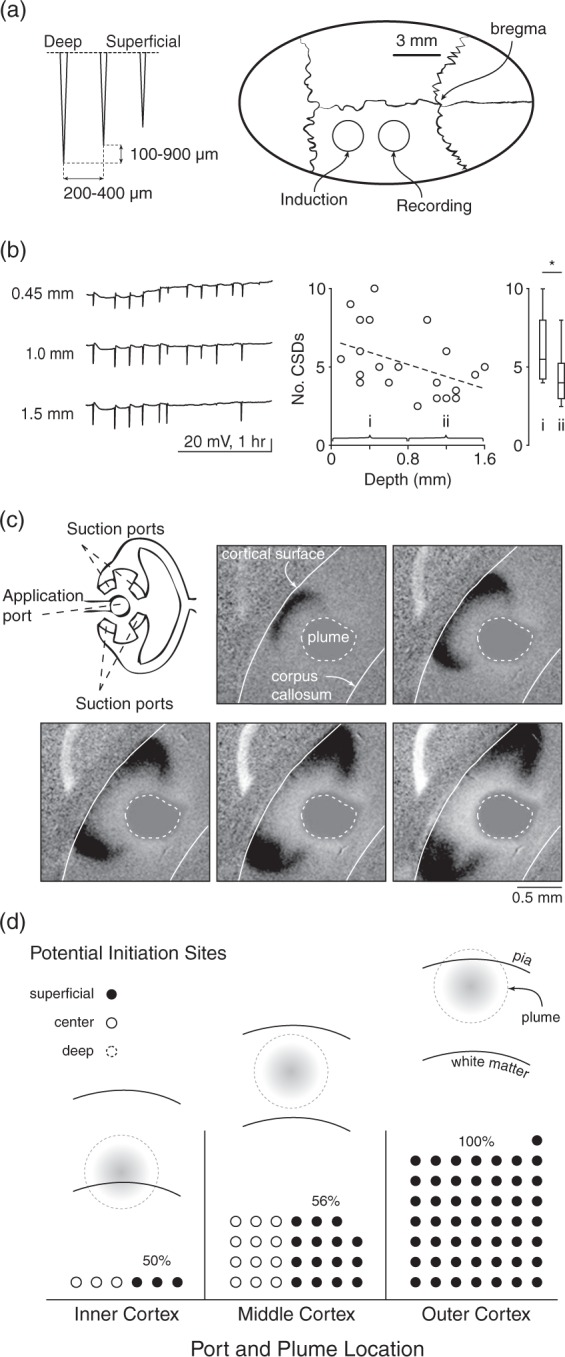
SD susceptibility and propagation vary by cortical depth. (a) Schematic shows depth electrode arrays and location of electrode and KCl stimulus placement in rat. (b) Example SD traces at 450, 1000, and 1500 µm below the cortical surface (all >3 mm away from stimulus) showing decreased incidence of SD at depth. Plot at right shows lower SD incidence by depth. Box plots show number of SD/hour at 1–800 µm and 800–1600 µm depth (p = 0.04, Student’s t-test); scatter plot shows all measurements. (Spearman’s rank order correlation R = −0.45, p = 0.02, n = 22 measurements in nine animals, five with triple electrode arrays, four with double electrode arrays). (c) Schematic shows microfluidic device with application and suction ports that allow delivery of a precisely sized plume of KCl to a mouse brain slice. Images show SD induction and propagation in the superficial and middle but not deep layers, to a plume centered between pia and white matter. (d) Preferential induction of SD in superficial layers. Location of plume was either in inner, middle, or outer third of cortex (schematics). SD could theoretically start in either inner, middle, or outer third of cortex for each experimental paradigm (dotted circle, solid circle, filled circle, respectively – each circle represents a single experiment). For plumes located in inner cortex, there was no induction in the inner layers; 50% of inductions were in middle (solid circle) and 50% were in outer cortex (filled circle). For plumes located in middle cortex, 56% were in outer cortex (the remainder were in middle cortex). For plumes located in outer cortex, 100% of SD were induced in outer cortex.
Though we spaced KCl stimulation at least 3 mm distant to the recording electrodes and in a separate burr hole, it is possible that the tropism for superficial layers in the above experiments was due to superficial KCl application. To account for this possibility, we used brain slice experiments where the size, location, and intensity of the stimulus, and the recording over different cortical layers, could be precisely controlled.
We used a microfluidic device with separate injection and suction ports that allowed us to control the location and shape of a plume of KCl in mouse brain slices (Figure 6(c)). The injection port center was aligned with either the upper, middle, or lower third of the cortical thickness, measured from pia to white matter. A typical SD induced from the middle location is shown in Figure 6(c). Despite the centered KCl perfusion, SD begins at the upper margins of the plume, and propagates preferentially in the superficial and not deep cortical layers. Figure 6(d) shows that for inductions in the middle of the slice, the majority of SD initiated in the upper layers, a minority in the middle layers, and none in the lower layers. For inductions in the upper layers, all SD were initiated in these layers. For inductions in the lower third, all SD were initiated in either the middle or upper third, rather than where the plume originated.
Discussion
The principal finding of this work is that SD are more heterogeneous – spatially, temporally, and by cortical location, than previously appreciated.
Preclinical implications
From Leão’s initial observation of a lack of propagation into retrosplenial granular regions, it has been known that SD susceptibility cannot be uniform across the cortex. Yet remarkably little is known about this susceptibility. We systematically tested SD incidence and propagation in four different cortical regions – retrosplenial, auditory, forelimb somatosensory, and primary visual – and found that both incidence and propagation varied.
SD incidence
The clear outlier was visual cortex, with a significantly higher incidence of SD, greater incidence of partial events, and significantly different hemodynamic correlates. The mechanisms underlying this differential susceptibility to repetitive SD are unclear. The highest neuronal density occurs in visual cortex in mouse34 and in human.35 For both mouse and human, visual cortex is statistically separable from all other regions by a unique relationship between cellular number and cortical volume.34,35 The clear outlier status in SD repetition would appear at least superficially consistent with the anatomical data. The cytoarchitectural separation of visual cortex might also provide an explanation for the frequent finding that SD did not propagate out of this region. The impression that emerges is that visual cortex has a different refractory period to other regions – whether because of cytoarchitectonic differences, hemodynamic response differences, or both – allowing the generation of more SD in a shorter period of time.
Note that our present results address the number of SD induced to a constant stimulus – they do not address absolute threshold of SD. While it might be intuitive to hypothesize that visual cortex would also have the lowest threshold for SD induction, we have found in separate work that this is not the case.36 When exposed to threshold concentrations of extracellular potassium, the first region to experience SD is somatosensory barrel cortex in the majority of cases. This shows that the threshold of SD is not equivalent to the ability to induce repetitive events – threshold and number are complementary and separable measures of susceptibility.
SD propagation
Though SD is considered an approximately concentric and isotropic phenomenon, we never observed an SD wave with either a smooth or circular wavefront. Moreover, maps of propagation showed fairly large alterations in velocity as the waves progressed over the cortex (Figure 4). To our knowledge, the only truly concentric and isotropic SD phenomena are generated in chick retina, which has a uniform, avascular, structure.9,37 This suggests that the heterogeneity of SD in cortex may be due to heterogeneity in structure, both cellular and vascular.
Overall, there was a striking difference in propagation of SD induced from four different regions (Figure 5). Two primary patterns emerge: SD with a high likelihood of propagating broadly (forepaw and auditory cortex induction) and SD with a much more local overall propagation (visual and retrosplenial induction).
We were able to confirm prior work showing that SD was less likely to propagate into retrosplenial cortex.10,13–15 However, it is noteworthy that there was no difficulty inducing SD in retrosplenial cortex – SD number was not significantly different from auditory and forepaw somatosensory inductions. It is possible that the interface between retrosplenial cortex and other regions, rather than retrosplenial cortex per se, constitutes the barrier to propagation. The relatively low “percent occupancy” of cortex outside retrosplenial cortex, for retrosplenial-induced SD (Figure 5(a)), would be consistent with such a hypothesis. It is interesting to note the similarity with visual cortex-induced SD; the high incidence of partial SD terminating within the borders of visual cortex suggesting a possible barrier at the interface of two regions.
We also observed an apparent preference for propagation through somatosensory barrel cortex, with directionality of propagation favoring barrel cortex for all inductions where barrel cortex was nearby (anterior, lateral, and posterior induction), and no directionality preference when barrel cortex was distant (medial induction). These data are in agreement with those of Eiselt et al.,13 who found that occipitally-induced SD propagated laterally before moving medially. Barrel cortex is both ethologically relevant and highly developed in rodent: it has high neuronal density34 and a complex columnar structure.38 Larger rises in extracellular K+ to a constant stimulus36 might also account for a relative propagation tropism.
Cytoarchitectural modulation of SD has recently been reported. Fujita et al.19 observed a decrease in propagation velocity at the interface of neocortex and paleocortex. Modulation of SD propagation correlated with relative astrocyte density, which was greater in paleocortex. It is possible that relative differences in astrocyte density also account for the differences we observed. Herculano-Houzel et al.34 counted both neurons and non-neuronal cells (dominated by astrocytes) in all cortical regions, and found the highest density of non-neuronal cells in retrosplenial cortex. This might account for the resistance to propagation into retrosplenial cortex (though it does not explain why SD induction was not disfavored). It is also interesting to note that visual cortex had both very high non-neuronal and neuronal density; speculatively, the high non-neuronal density might contribute to SD recovery, allowing the higher rates of SD in this region.
It is likely that relative glial density is not the only contributor to different SD susceptibility and propagation. Cortical myelin suppresses SD propagation,20 suggesting an effect of structural complexity beyond simple cellular density. The structural complexity of barrel cortex may account for its greater susceptibility to SD induction than other regions.36 It would also be surprising if the functional characteristics of cortex, mediated by the complement of receptors and channels in different regions, were not involved.
There was an apparent modulation of SD propagation by vascular structures, consistent with reports in both lissencephalic19 and gyrencephalic39 brain. We observed constraint or stoppage of propagation by large cortical veins, most prominently when parallel rather than perpendicular to the advancing wavefront. Given this geometry, we agree with prior hypotheses that vessels served (at least in part) as physical barriers to propagation.19,39
In addition to possible cytoarchitectonic and vascular modulation of propagation, there was a clear modulation by prior SD, suggestive of an influence of relative and absolute refractory periods. The most dramatic example was the significant decrement in SD velocity between first and subsequent waves (Figures 2 and 4). This effect was long-lasting, as we observed reduced velocity SD for the duration of the experiments. As a possible mechanism, there is long-lasting tissue depolarization after SD, associated with a second direct current shift in extracellular field potential26 lasting over an hour, and membrane depolarization at least 30 min after the passage of the SD wave.40 On a shorter time scale but also suggestive of refractory phenomena were SD that alternated location with prior SD, and spiral SD (Figure 4(c) and (e)). In addition, the alternation of “full” and “partial” SD (Figure 4(b)) may also be due to relative refractory periods: SD arising and propagating in tissue that has not fully repolarized may not have the capacity to propagate as far, or to propagate across relative barriers (cytoarchitectonic boundaries, vessels, or other).
It is worth noting that despite its lissencephalic nature, rodent cortex supported highly complex propagation patterns, including spiral waves. This kind of complex SD phenomenology has been reported in gyrencephalic cortex, and the structural nature of gyrencephalic cortex advanced as an explanation for the complexity.39 While our data do not in any way rule out influences of gyration, they show that it is not necessary for the generation of complex SD phenotypes. This should not be surprising, as spiral waves are observed in the even simpler retina,41 and previous work in rodents has suggested such phenomenology.42 From a theoretical standpoint, circling or spiral waves can be explained by refractory periods in any excitable medium43 – they do not require structural complexity.
Differential susceptibility by cortical depth
Leão first showed that SD was more easily induced with electrical stimulation, and propagated faster, in the superficial cortical layers.12,44 Later work with brain slices showed that SD propagates preferentially in superficial cortical layers.17 However, other work in vivo has suggested preferential propagation in lower cortical layers, and a relative barrier to SD propagation between superficial and deep layers.45 In hippocampus, distinct propagation has been demonstrated in dendritic versus cellular layers16 that might have correlates in the cortex.
We therefore revisited the issue of SD initiation and propagation by depth, with in vivo and in vitro recordings. Both sets of experiments favor superficial propagation of SD: the total SD count was higher in superficial layers in vivo, and preferential spread in superficial layers could actually be observed in vitro. We also directly addressed SD susceptibility by depth in vitro. We were able to demonstrate that SD tended to be induced superficially even when a KCl plume was delivered to deeper layers. There are many possible mechanisms for this tropism, including neuronal, glial, and vascular density, structural complexity, and repertoire of conductances. While it is likely that many factors play a role, we suspect that the enrichment of dendritic structures, with their associated excitatory conductances, may be important.
Methodological issues in SD research
Given the different susceptibility and propagation at different cortical locations, it is important to specify (ideally with anatomical coordinates) the location of induction and recording. As susceptibility varies by depth, this applies not only to location at the cortical surface, but location within cortex.
It is also important to consider the temporal order of SD in analysis and reporting. The first SD is significantly different from subsequent events, and SD can easily be induced during surgical preparation, even in experienced hands. It is likely that much analysis and reporting of SD has pooled first and subsequent SD, with a consequent “blurring” of characterization. We recommend that monitoring for SD commences with the beginning of the surgical preparation, and that all reporting of SD take into account the effect of prior SD as a potential modulator.
Finally, the large spatiotemporal heterogeneity of SD can clearly create ambiguity when point measurements (electrodes, biosensors) are used. Clear specification of location in x, y, and z planes is helpful, and for repetitive events the possibility of eccentric waveforms generating difficult-to-interpret phenotypes must be entertained. Ideally, 2- and 3-D techniques can be combined with point measurements to better account for heterogeneity.
Potential limitations
We relied primarily on optical measurement of SD, due to its ability to generate a continuous two-dimensional map of propagation. It is well known that SD can alter neurovascular coupling2,3,8,25,26,46; thus it can be asked whether the primarily hemodynamic measures we used faithfully represent the depolarization of SD. It is also known that the vascular correlates in mouse (our primary subject) vary significantly from other animals,3,47 potentially introducing bias into our measurements. However, though the optical signal is complex, multiphasic, and varies with number of SD, it remains a large signal that can be easily distinguished from ongoing activity. It also appears to faithfully report depolarization as recorded with electrodes or voltage sensitive dye,3,25,39,47,48 in both lissencephalic and gyrencephalic species. And while mouse has a more pronounced hypoperfusion phase than other species, it retains the same multiphasic optical profile as other species, and the same relation of that profile to depolarization.3 The main caveat is that most (but not all) of this data come from “full” SD, leaving the possibility that optical and electrical recordings do not correspond as well in “partial” SD scenarios. Ultimately this question can be resolved with combined distributed electrical recordings33 or ideally with voltage sensitive dye.48
Clinical/translational implications
Clinically, SD is heterogeneous. Though migraine aura can be stereotyped, it can also vary greatly even within the same subject.49,50 SD recorded from humans with brain injury show even greater variability,2,4,8 likely due in part to the diverse nature of injury, but here again there is also large intra-subject variability. It is likely that incidence, repetition rate, and pattern and extent of SD propagation vary by both cortical region and depth in humans as well as experimental animals.10,13–15,17 Differential susceptibility to SD can explain why the migraine aura arises where it does, and can suggest territories at risk in humans.36 An understanding of the mechanisms that generate this differential susceptibility is a major goal for future SD research, as it offers the promise of modulating SD therapeutically.
Funding
The author(s) disclosed receipt of the following financial support for the research, authorship, and/or publication of this article: This work was supported by the National Institutes of Health (NS 085413; KCB; Intramural Research Program, CC; JCC), Department of Defense (CDMRP PR 130373), National Science Foundation (DMS 0635561; JCC).
Declaration of conflicting interests
The author(s) declared no potential conflicts of interest with respect to the research, authorship, and/or publication of this article.
Authors’ contributions
KCB took part in the study conception; DK, JZ, YTT, VBB, and KCB in experimental design; DK, JZ, CAS, YTT, VBB, and SM performed experiments; DK, JZ, JJT, CAS, YTT, VBB, JCC, and KCB took part in the analysis;: DK, JZ, JJT, CAS, YTT, VBB, JCC, SM, JS, YSJ, and KCB wrote the manuscript.
References
- 1.Pietrobon D, Moskowitz MA. Chaos and commotion in the wake of cortical spreading depression and spreading depolarizations. Nat Rev Neurosci 2014; 15: 379–393. [DOI] [PubMed] [Google Scholar]
- 2.Dreier JP. The role of spreading depression, spreading depolarization and spreading ischemia in neurological disease. Nat Med 2011; 17: 439–447. [DOI] [PubMed] [Google Scholar]
- 3.Ayata C, Lauritzen M. Spreading depression, spreading depolarizations, and the cerebral vasculature. Physiol Rev 2015; 95: 953–993. [DOI] [PMC free article] [PubMed] [Google Scholar]
- 4.Lauritzen M, Dreier JP, Fabricius M, et al. Clinical relevance of cortical spreading depression in neurological disorders: migraine, malignant stroke, subarachnoid and intracranial hemorrhage, and traumatic brain injury. J Cereb Blood Flow Metab 2011; 31: 17–35. [DOI] [PMC free article] [PubMed] [Google Scholar]
- 5.Charles B. Cortical spreading depression-new insights and persistent questions. Cephalalgia 2009; 29: 1115–1124. [DOI] [PMC free article] [PubMed] [Google Scholar]
- 6.Pietrobon D, Moskowitz MA. Pathophysiology of migraine. Annu Rev Physiol 2013; 75: 365–391. [DOI] [PubMed] [Google Scholar]
- 7.Lauritzen Pathophysiology of the migraine aura. The spreading depression theory. Brain 1994; 117: 199–210. [DOI] [PubMed] [Google Scholar]
- 8.Dreier JP, Reiffurth C. The stroke-migraine depolarization continuum. Neuron 2015; 86: 902–922. [DOI] [PubMed] [Google Scholar]
- 9.Martins-Ferreira H, de Castro GO. Light-scattering changes accompanying spreading depression in isolated retina. J Neurophysiol 1966; 29: 715–726. [DOI] [PubMed] [Google Scholar]
- 10.Leao AAP. Spreading depression of activity in cerebral cortex. J Neurophysiol 1944; 7: 359–390. [DOI] [PubMed] [Google Scholar]
- 11.Leao AAP. Pial circulation and spreading depression of activity in cerebral cortex. J Neurophysiol 1944; 7: 391–396. [Google Scholar]
- 12.Leao AAP, Morison RS. Propagation of spreading cortical depression. J Neurophysiol 1945; 8: 33–45. [Google Scholar]
- 13.Eiselt M, Giessler F, Platzek D, et al. Inhomogeneous propagation of cortical spreading depression-detection by electro- and magnetoencephalography in rats. Brain Res 2004; 1028: 83–91. [DOI] [PubMed] [Google Scholar]
- 14.Chen S, Li P, Luo W, et al. Time-varying spreading depression waves in rat cortex revealed by optical intrinsic signal imaging. Neurosci Lett 2006; 396: 132–136. [DOI] [PubMed] [Google Scholar]
- 15.Fifkova E. Spreading EEG depression in the neo-, paleo-, and archicortical structures of the brain of the rat. Physiol Bohemoslov 1964; 13: 1–15. [PubMed] [Google Scholar]
- 16.Herreras O, Somjen GG. Propagation of spreading depression among dendrites and somata of the same cell population. Brain Res 1993; 610: 276–282. [DOI] [PubMed] [Google Scholar]
- 17.Basarsky TA, Duffy SN, Andrew RD, et al. Imaging spreading depression and associated intracellular calcium waves in brain slices. J Neurosci 1998; 18: 7189–7199. [DOI] [PMC free article] [PubMed] [Google Scholar]
- 18.Bogdanov VB, Multon S, Chauvel V, et al. Migraine preventive drugs differentially affect cortical spreading depression in rat. Neurobiol Dis 2011; 41: 430–435. [DOI] [PubMed] [Google Scholar]
- 19.Fujita S, Mizoguchi N, Aoki R, et al. Cytoarchitecture-dependent decrease in propagation velocity of cortical spreading depression in the rat insular cortex revealed by optical imaging. Cereb Cortex 2015; 26: 1580–1589. [DOI] [PubMed] [Google Scholar]
- 20.Merkler D, Klinker F, Jürgens T, et al. Propagation of spreading depression inversely correlates with cortical myelin content. Ann Neurol 2009; 66: 355–365. [DOI] [PubMed] [Google Scholar]
- 21.Guide for the care and use of laboratory animals, 8th ed. National Academies Press, https://grants.nih.gov/grants/olaw/Guide-for-the-Care-and-use-of-laboratory-animals.pdf#page=1&zoom=auto,-144,648 (accessed 27 May2016).
- 22.Kilkenny C, Browne WJ, Cuthill IC, et al. Improving bioscience research reporting: the ARRIVE Guidelines for Reporting Animal Research. PLoS Biol 2010; 8: e1000412. [DOI] [PMC free article] [PubMed] [Google Scholar]
- 23.Brennan KC, Romero Reyes M, Lopez-Valdes HE, et al. Reduced threshold for cortical spreading depression in female mice. Ann Neurol 2007; 61: 603–606. [DOI] [PubMed] [Google Scholar]
- 24.Eikermann-Haerter K, Dileköz E, Kudo C, et al. Genetic and hormonal factors modulate spreading depression and transient hemiparesis in mouse models of familial hemiplegic migraine type 1. J Clin Invest 2009; 119: 99–109. [DOI] [PMC free article] [PubMed] [Google Scholar]
- 25.Brennan KC, Beltran-Parrazal L, Lopez Valdes HE, et al. Distinct vascular conduction with cortical spreading depression. J Neurophysiol 2007; 97: 4143–4151. [DOI] [PubMed] [Google Scholar]
- 26.Chang JC, Shook LL, Biag JD, et al. Biphasic direct current shift, hemoglobin desaturation, and neurovascular uncoupling in cortical spreading depression. Brain 2010; 133: 996–1012. [DOI] [PMC free article] [PubMed] [Google Scholar]
- 27.Kaufmann D, Bates EA, Yagen B, et al. sec-Butylpropylacetamide (SPD) has antimigraine properties. Cephalalgia 2015. DOI: 10.1177/0333102415612773. [DOI] [PMC free article] [PubMed] [Google Scholar]
- 28.Tang YT, Mendez JM, Theriot JJ, et al. Minimum conditions for the induction of cortical spreading depression in brain slices. J Neurophysiol 2014; 112: 2572–2579. [DOI] [PMC free article] [PubMed] [Google Scholar]
- 29.Tang YT, Kim J, López-Valdés HE, et al. Development and characterization of a microfluidic chamber incorporating fluid ports with active suction for localized chemical stimulation of brain slices. Lab Chip 2011; 11: 2247–2254. [DOI] [PMC free article] [PubMed] [Google Scholar]
- 30.Frostig RD, Lieke EE, Ts’o DY, et al. Cortical functional architecture and local coupling between neuronal activity and the microcirculation revealed by in vivo high-resolution optical imaging of intrinsic signals. Proc Natl Acad Sci U S A 1990; 87: 6082–6086. [DOI] [PMC free article] [PubMed] [Google Scholar]
- 31.Hillman EMC. Optical brain imaging in vivo: techniques and applications from animal to man. J Biomed Opt 2007; 12: 051402–051428. [DOI] [PMC free article] [PubMed] [Google Scholar]
- 32.Mané M, Müller M. Temporo-spectral imaging of intrinsic optical signals during hypoxia-induced spreading depression-like depolarization. PloS One 2012; 7: e43981. [DOI] [PMC free article] [PubMed] [Google Scholar]
- 33.Theriot JJ, Toga AW, Prakash N, et al. Cortical sensory plasticity in a model of migraine with aura. J Neurosci 2012; 32: 15252–15261. [DOI] [PMC free article] [PubMed] [Google Scholar]
- 34.Herculano-Houzel S, Watson C, Paxinos G. Distribution of neurons in functional areas of the mouse cerebral cortex reveals quantitatively different cortical zones. Front Neuroanat 2013; 7: 35. [DOI] [PMC free article] [PubMed] [Google Scholar]
- 35.Ribeiro PFM, Ventura-Antunes L, Gabi M, et al. The human cerebral cortex is neither one nor many: neuronal distribution reveals two quantitatively different zones in the gray matter, three in the white matter, and explains local variations in cortical folding. Front Neuroanat 2013; 7: 28. [DOI] [PMC free article] [PubMed] [Google Scholar]
- 36.Bogdanov VB, Middleton NA, Theriot JJ, et al. Susceptibility of Primary Sensory Cortex to Spreading Depolarizations. J Neurosci Off J Soc Neurosci 2016; 36: 4733–4743. [DOI] [PMC free article] [PubMed] [Google Scholar]
- 37.Martins-Ferreira H, Nedergaard M, Nicholson C. Perspectives on spreading depression. Brain Res Brain Res Rev 2000; 32: 215–234. [DOI] [PubMed] [Google Scholar]
- 38.Petersen CCH. The functional organization of the barrel cortex. Neuron 2007; 56: 339–355. [DOI] [PubMed] [Google Scholar]
- 39.Santos E, Scholl M, Sanchez-Porras R, et al. Radial, spiral and reverberating waves of spreading depolarization occur in the gyrencephalic brain. Neuroimage 2014; 99: 244–255. [DOI] [PubMed] [Google Scholar]
- 40.Sawant PM, Suryavanshi P, Mendez JM, et al. Mechanisms of neuronal silencing after cortical spreading depression. Cereb Cortex 2015. (in Press). [DOI] [PMC free article] [PubMed] [Google Scholar]
- 41.Martins-Ferreira H, De Oliveira Castro G, Struchiner CJ, et al. Circling spreading depression in isolated chick retina. J Neurophysiol 1974; 37: 773–784. [DOI] [PubMed] [Google Scholar]
- 42.Shibata M, Bures J. Reverberation of cortical spreading depression along closed-loop pathways in rat cerebral cortex. J Neurophysiol 1972; 35: 381–388. [DOI] [PubMed] [Google Scholar]
- 43.Gerhardt M, Schuster H, Tyson JJ. A cellular automation model of excitable media including curvature and dispersion. Science 1990; 247: 1563–1566. [DOI] [PubMed] [Google Scholar]
- 44.Leao AA. The slow voltage variation of cortical spreading depression of activity. Electroencephalogr Clin Neurophysiol 1951; 3: 315–321. [DOI] [PubMed] [Google Scholar]
- 45.Richter F, Lehmenkuhler A. Spreading depression can be restricted to distinct depths of the rat cerebral cortex. Neurosci Lett 1993; 152: 65–68. [DOI] [PubMed] [Google Scholar]
- 46.Piilgaard H, Lauritzen Persistent increase in oxygen consumption and impaired neurovascular coupling after spreading depression in rat neocortex. J Cereb Blood Flow Metab 2009; 29: 1517–1527. [DOI] [PubMed] [Google Scholar]
- 47.Ayata C, Shin HK, Salomone S, et al. Pronounced hypoperfusion during spreading depression in mouse cortex. J Cereb Blood Flow Metab 2004; 24: 1172–1182. [DOI] [PubMed] [Google Scholar]
- 48.Farkas E, Pratt R, Sengpiel F, et al. Direct, live imaging of cortical spreading depression and anoxic depolarisation using a fluorescent, voltage-sensitive dye. J Cereb Blood Flow Metab 2008; 28: 251–262. [DOI] [PMC free article] [PubMed] [Google Scholar]
- 49.Schott GD. Exploring the visual hallucinations of migraine aura: the tacit contribution of illustration. Brain 2007; 130: 1690–1703. [DOI] [PubMed] [Google Scholar]
- 50.Hansen JM, Baca SM, Vanvalkenburgh P, et al. Distinctive anatomical and physiological features of migraine aura revealed by 18 years of recording. Brain 2013; 136: 3589–3595. [DOI] [PubMed] [Google Scholar]
- 51.Chang JC, Brennan KC and Chou T. Tracking monotonically advancing boundaries in image sequences using graph cuts and recursive kernel shape priors. IEEE Trans Medl Imaging 2012; 31(5): 1008–1020. [DOI] [PMC free article] [PubMed]
- 52.Chang JC, Chou T. Iterative graph cuts for image segmentation with a nonlinear statistical shape prior. J Math Imaging Vis 2014; 49(1): 87–97. [DOI] [PMC free article] [PubMed]