Direct Estimation of Tracer-Kinetic Parameter Maps from Highly Undersampled Brain DCE-MRI

Abstract

Purpose

To develop and evaluate a T1-weighted dynamic contrast enhanced (DCE) MRI methodology where tracer-kinetic (TK) parameter maps are directly estimated from undersampled (k,t)-space data.

Methods

The proposed reconstruction involves solving a non-linear least squares optimization problem that includes explicit use of a full forward model to convert parameter maps to (k,t)-space, utilizing the Patlak TK model. The proposed scheme is compared against an indirect method that creates intermediate images via parallel imaging and compressed sensing prior to TK modeling. Thirteen fully-sampled brain tumor DCE-MRI scans with 5 sec temporal resolution are retrospectively undersampled at rates R=20, 40, 60, 80, and 100 for each dynamic frame. TK maps are quantitatively compared based on root mean-squared-error (rMSE), and Bland-Altman analysis. The approach is also applied to four prospectively R=30 undersampled whole-brain DCE-MRI data sets.

Results

In the retrospective study, the proposed method performed statistically better than indirect method at R≥80 for all thirteen cases. This approach provided restoration of TK parameter values with less errors in tumor regions-of-interest, an improvement compared to a state-of-the-art indirect method. Applied prospectively, the proposed method provided whole-brain high-resolution TK maps with good image quality.

Conclusion

Model-based direct estimation of TK maps from k,t-space DCE-MRI data is feasible and is compatible up to 100-fold undersampling.

Introduction

Brain dynamic contrast enhanced (DCE) MRI is used to measure neurovascular parameters such as blood-brain-barrier (BBB) permeability in a variety of conditions including brain tumor (1,2), multiple sclerosis (3,4), and Alzheimer disease (5). DCE-MRI involves collecting a series of T₁-weighted images during the administration of a T₁-shortening contrast agent (6,7). TK modeling is then performed on the dynamic images to estimate physiological parameters, such as vascular permeability (K^trans), fractional plasma volume (v_p), and extravascular-extracellular volume fraction (v_e) (8,9). The anatomic dynamic images are primarily used to derive the TK maps (2,10–12).

For many applications, current DCE-MRI with Nyquist sampling is unable to simultaneously provide high spatio-temporal resolution and adequate volume coverage. Compressed sensing (13) and parallel imaging (14,15) based schemes have been proposed to accelerate acquisition process, primarily to achieve better spatial resolution and coverage while maintaining the same temporal resolution. Notably, Lebel et al. (16) used a temporal high pass filter and multiple spatial sparsity constraints to achieve an undersampling rate (R) of 36×, and showed excellent quality of anatomic images in brain tumor cases. A recent pilot study in brain tumor patients indicated that this approach performs superior to conventional techniques with no apparent loss of diagnostic information (17). The works of Feng et al. (18), Chandarana et al. (19), Rosenkrantz et al. (20), used a golden-angle radial sampling pattern, compressed sensing, and parallel imaging to achieve a comparable acceleration rate of 19.1 to 28.7. These studies showed improved resolution and reduced motion sensitivity in breast, liver, and prostate DCE-MRI, compared to either parallel imaging alone or coil-by-coil compressed sensing alone. We will refer to these techniques as “indirect” methods, since the anatomic image series are reconstructed first, followed by a separate step for TK parameter fitting on a voxel-by-voxel basis.

In this work, we propose a framework for “direct” estimation of TK parameter maps from fully-sampled or undersampled (k,t)-space data. We employ a full forward model that converts the TK maps to (k,t)-space, and we pose the estimation of TK maps as an error minimization problem. Our approach is motivated by two factors: 1) spatial TK parameter maps have much lower dimensionality than those of dynamic image series (2-4 parameters, compared to 50-100 time points, per voxel), and 2) TK model-based reconstruction directly exploits what is known about contrast agent kinetics. These allow for robust parameter estimation from an information theoretic perspective, and has the potential to provide the most accurate restoration of TK parameter values, and allow for the highest acceleration.

Model-based direct reconstruction has been previously explored in other applications such as MRI relaxation parameter estimation (21–26), TK parameter estimation in PET (27–29), and TK parameter estimation in MRI (30,31). Notably, for MRI relaxation parameter estimation, Sumpf et al. (24) used a model-based nonlinear inverse reconstruction to estimate T2 maps from highly undersampled spin-echo MRI data; Zhao et al. (25) estimated T1 parameters directly from undersampled MRI data with a sparsity constraint on the parameter maps. For dynamic PET imaging, Kamasak et al. (28) directly estimated TK parameter images from dynamic PET data using a kinetic model-based reconstruction optimization; Lin et al. (29) used a sparsity constrained mixture model to estimate TK parameters from dynamic PET data, and evaluated with both simulated and experimental PET data.

For DCE MRI parameter mapping, Felsted et al. (30) proposed to use a model-based reconstruction algorithm to solve TK parameters directly from undersampled MRI k-space with a modified gradient descent algorithm. An undersampling factor of R=4 was demonstrated on simulated data; Dikaios et al. (31) proposed a Bayesian inference framework to directly estimate TK maps from undersampled MRI data, and achieved 8× acceleration in phantom and in-vivo prostate cancer data.

While the prior studies demonstrate promise, the full potential of TK model based reconstruction has lacked validation, both at higher undersampling rates, or with prospectively undersampled data from patients. In this study, we explore the maximum potential benefit of the direct TK estimation by testing very high undersampling rates. We validate the approach using retrospective undersampling of fully-sampled data and using prospectively undersampled DCE data sets from brain tumor patients. Compared to prior work, we are able to demonstrate much higher undersampling rates (up to 100×) in the retrospective study, using a more efficient gradient-based algorithm. We use quantitative evaluation (root Mean Square Error (rMSE) in TK parameters) to provide a systematic comparison against a state-of-the-art compressed sensing method that uses spatial and temporal sparsity constraints in 13 brain tumor patients. We also uniquely provide a prospective in-vivo study showing that whole-brain coverage with high spatial resolution can be achieved to capture complete pathological information. We demonstrate the potential of direct reconstruction to enable “parameter-free” reconstruction, when no sparsity constraints are added.

Theory

Direct TK Mapping

We propose to integrate TK modeling, specifically the Patlak model, into the image reconstruction process. Figure 1 illustrates the forward model that relates TK parameter maps to undersampled (k,t)-space. We use the vector r ∈ (x,y,z) to represent image domain spatial coordinates, k ∈ (k_x,k_y,k_z)to represents k-space coordinates; t, c are the time and coil dimensions. The variables beneath the arrows of each step are known or predetermined. The steps indicated (above the arrows) in Figure 1 are explained below:

1. Contrast agent concentration over time CA(r,t) is assumed to follow the Patlak model:

   $$\mathit{\text{CA}}(\mathit{r},t)=K^{\mathit{\text{trans}}}(\mathit{r})\underset{0}{\overset{t}{\int }}{C}_p(\tau )\mathrm{d}\tau +v_p(\mathit{r})C_p(t)$$ [Eqn 1]

   where C_p(t) is the arterial input function (AIF). In this work, we used a population-based AIF from (32). Notice that the AIF requires specifying a delay time. This is estimated from the k-space origin, which is acquired in every time frame, and has shown to accurately detect the time of contrast bolus arrival (33). We assume that the Patlak is appropriate for all voxels in the imaging volume. We have observed that image regions outside of vessels and tumor typically experience no enhancement during the DCE-MRI acquisition which results in a fit to v_p=0, K^trans=0.

2. Dynamic anatomic images s(r,t) are related to CA(r,t) by the steady state spoiled gradient echo (SPGR) signal equation:

   $$s(\mathit{r},t)=\frac{M_0(\mathit{r})sin\alpha (1-e^{-\mathit{\text{TR}}\cdot [R_1(\mathit{r},0)+\mathit{\text{CA}}(\mathit{r},t)\cdot r_1]})}{1-cos\alpha e^{-\mathit{\text{TR}}\cdot [R_1(\mathit{r},0)+\mathit{\text{CA}}(\mathit{r},t)\cdot r_1]}}+[s(\mathit{r},0)-\frac{M_0(\mathit{r})sin\alpha (1-e^{-\mathit{\text{TR}}\cdot R_1(\mathit{r},0)})}{1-cos\alpha e^{-\mathit{\text{TR}}\cdot R_1(\mathit{r},0)}}]$$ [Eqn 2]

   where TR is the repetition time, α is the flip angle, r₁ is the contrast agent relaxivity, R₁(r,0) and M₀(r) are the pre-contrast R₁ (reciprocal of T₁) and the equilibrium longitudinal magnetization that are estimated from a T₁ mapping sequence. In this work, we used DESPOT1 (34) immediately prior to the DCE-MRI scan. s(r,0) is the pre-contrast first-frame, which is fully-sampled in this work. The bracketed [] term resolves differences between the pre-contrast signal and the predicted pre-contrast signal based on the baseline T1 and M0 maps (from DESPOT1 sequences) (35).

3. The undersampled raw (k,t)-space data S(k,t,c) is related to s(r,t) by the coil sensitivities C(r,c), and undersampling Fourier transform (F_u):

   $$S(\mathit{k},t,c)=F_{u}C(\mathit{r},c)s(\mathit{r},t)$$ [Eqn 3]

   In this work, C(r,c) is estimated from time averaged data using the standard root sum-of-squares method (14). The image phase information is assumed to be captured by the complex-valued sensitivity maps.

Figure 1.

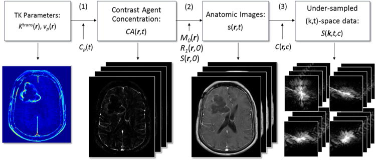
DCE-MRI forward model flowchart illustrating the conversion from TK parameter maps to undersampled (k,t)-space. Patlak model is used to convert TK parameter maps to contrast concentration over time, after which the T₁-weighted signal equation is used to obtain the dynamic anatomic images. Fourier transform, sensitivity maps and sampling pattern connect anatomic images to multi-coil (k,t)-space measurements.

Combining Eqn 1-3, we reach a general function f to denote the relationship between TK maps K^trans(r),v_p(r) and undersampled (k,t)-space S(k,t,c).

$$S(\mathit{k},t,c)=f(K^{\mathit{\text{trans}}}(\mathit{r}),v_p(\mathit{r});C_p(t),\mathit{\text{TR}},\alpha ,R_1(\mathit{r},0),M_0(\mathit{r}),r_1,C(\mathit{r},c))$$ [Eqn 4]

where C_p(t),TR,α,R₁(r,0),M₀(r), r₁,C(r,c) are variables that are known or pre-determined as mentioned above. We solve for the unknown K^trans(r), v_p(r) via least-square optimization, formulated as follows:

$$(K^{\mathit{\text{trans}}}(\mathit{r}),v_p(\mathit{r}))=\underset{K^{\mathit{\text{trans}}}(\mathit{r}),v_p(\mathit{r})}{argmin}{\Vert S(\mathit{k},t,c)-f(K^{\mathit{\text{trans}}}(\mathit{r}),v_p(\mathit{r}))\Vert }_2^2$$ [Eqn 5]

This nonlinear optimization problem is solved by a quasi-Newton limited-memory Broyden-Fletcher-Goldfarb-Shannon (l-BFGS) method (36), where K^trans(r) and v_p(r) are solved alternatingly. The details of the optimization algorithm and gradient calculation are provided in Appendix I.

Direct reconstruction by itself is “parameter-free”. This is in contrast to compressed sensing based algorithms that require tuning of one or more regularization parameters. It is possible to incorporate additional spatial sparsity constraints on the TK maps themselves. In this work, we test the potential value of adding a spatial ‘db2’ wavelet constraint (Ψ) to the parameter maps. The optimization problem with sparsity constraint is formulated as follows:

$$({\mathit{k}}^{\mathit{\text{trans}}}(\mathit{r}),v_p(\mathit{r}))\underset{K^{\mathit{\text{trans}}}(\mathit{r}),v_p(\mathit{r})}{argmin}{\Vert S(\mathit{K},t,c)-f(K^{\mathit{\text{trans}}}(\mathit{r}),v_p(\mathit{r}))\Vert }_2^2+{\lambda }_1{\Vert \psi K^{\mathit{\text{trans}}}(\mathit{r})\Vert }_1+{\lambda }_2{\Vert \psi v_p(\mathit{r})\Vert }_1$$ [Eqn 6]

We provide source code, along with sample datasets, and scripts that generate several of the figures from this manuscript (37), Repository: https://github.com/usc-mrel/DCE_direct_recon; Release 1: https://doi.org/10.5281/zenodo.154058

Indirect TK Mapping

Current state-of-the-art methods for highly accelerated DCE involve reconstructing intermediate images prior to TK modeling. These indirect methods are the most relevant alternatives to direct TK modeling and serve as a performance benchmark. A basic model for indirect reconstruction solves the minimization problem in [Eqn 7], where the final image, s(r,t), remains consistent with acquired (k,t)-space data S(k,t,c), yet is sparse in the temporal finite differences (V) domain and spatial wavelet domain (Ψ).

$$s(\mathit{r},t)=\underset{s(\mathit{r},\mathit{t})}{argmin}{\Vert S(\mathit{k},t,c)-F_{u}C(\mathit{r},\mathrm{c})s(\mathit{r},t)\Vert }_2^2+{\lambda }_1{\Vert V_s(\mathit{r},t)\Vert }_1+{\lambda }_2{\Vert \psi s(\mathit{r},t)\Vert }_1$$ [Eqn 7]

The image is related to the acquired data using known coil sensitivities C(r,c) and the undersampling Fourier transform F_u. TK modeling (e.g. using a Patlak model) is performed in a last step to estimate the spatial TK maps (e.g. K^trans(r), v_p(r)) from s(r,t). This optimization problem was solved by an efficient augmented Lagrangian method, alternating direction methods of multipliers (ADMM) (38), to get the anatomic images.

Methods

Digital Phantom

We simulated realistic DCE-MRI data using a digital phantom with known TK parameter maps and using the Patlak TK model. We used a process identical to Ref. (39), where the segmentation is extracted from patient data. Realistic sensitivity maps were used, and noise was added to each channel according to noise covariance matrix estimated from the patient data. A pre-contrast white-matter SNR level of 20 was chosen to mimic the SNR level in actual DCE data sets.

We retrospectively undersampled k,t-space with rates R of 20× to 100×. Ten noise realizations were generated for each R. Undersampling was in the k_x -k_y plane, simulating the k_y-k_z plane as in a prospectively undersampled 3D case, using a randomized golden-angle radial sampling pattern (40,41). Detailed description and the videos of the undersampling strategies can be found in and the supporting materials. Direct and indirect methods were used to generate the TK parameters from both fully-sampled and undersampled data. TK map rMSE were computed over an ROI containing the entire tumor boundary.

In-Vivo Retrospective Evaluation

We reviewed 110 fully-sampled DCE-MRI raw data sets from patients with known or suspected brain tumor, receiving a routine brain MRI with contrast on a clinical 3T scanner (HDxt, GE Healthcare, Waukesha, WI). The data sets were from patients receiving routine brain MRI with contrast (including DCE-MRI) at our Institution, and the demographics reflect our local patient population. Our Institution follows standard exclusion criteria for MRI with Gadolinium-based contrast (42,43) which includes: medically unstable, renal impairment, cardiac pacemaker, internal ferromagnetic device that is contraindicated for use in MRI, claustrophobia, and any other condition that would compromise the scan with reasonable safety. The retrospective study protocol was approved by our Institutional Review Board.

The sequence was based on a 3D Cartesian fast spoiled gradient echo sequence (SPGR) with FOV: 22×22×4.2cm³, spatial resolution: 0.9×1.3×7.0mm³, temporal resolution: 5s, 50 time frames, and 8 receiver coils. The flip angle is 15°, and TE is 1.3ms, TR is 6ms. DESPOT1 was performed before the DCE sequence, where three images with flip angle of 2°, 5°, 10° were acquired to estimate T₁ and M₀ maps before the contrast arrival. The contrast agent, Gadobenate dimeglumine (MultiHance Bracco Inc., which has relaxivity r₁ =4.39 s^-1mM^-1 at 37°C at 3 Tesla (44)) was administered with a dose of 0.05 mMol/kg, followed by a 20 ml saline flush in the left arm by intravenous injection.

Of the 110 cases, we found 18 that had visible tumor larger than 1cm by bidirectional assessment. TK parameter maps K^trans and v_P were calculated from the fully-sampled images, and TK model fitting error was computed by taking the l₂ norm between the contrast concentration curves from fully-sampled images, CA(r,t), and the fitted concentration curves generated from the TK parameter maps, $\widehat{\mathit{\text{CA}}}(\mathit{r},t)$. We then examined the Patlak modeling error, defined as:

$$\frac{{\Vert \widehat{\mathit{\text{CA}}}(\mathit{r},t)-\mathit{\text{CA}}(\mathit{r},t)\Vert }_2^2}{{\Vert \mathit{\text{CA}}(\mathit{r},t)\Vert }_2^2}\times 100\%$$ [Eqn 8]

Of the 18 cases with visible tumor larger than 1cm, 13 cases had Patlak modelling error less than 1%, suggesting that the Patlak model with the population AIF was appropriate. The analysis below was performed on the 13 cases which were fully-sampled, had at least one tumor larger than 1cm, and for whom the Patlak model fitted the fully-sampled data with less than 1% error

For each selected case, three sets of TK maps were generated from: 1) standard Fourier reconstruction of fully sampled data. These served as the gold standard reference maps. 2) Direct reconstruction method using retrospective undersampling; 3) Indirect reconstruction using retrospective undersampling. We examined R of 20× to 100×, with at increments of 20×. For each R, 10 realizations of the sampling pattern were generated using a different initial angle in the randomized golden-angle radial scheme. This effectively creates multiple noise realizations, since there is almost no overlap in the (k,t) sampling pattern (except for the one sample at the k-space origin, which is included in every sampling scheme at every undersampling factor).

For indirect method [Eqn 7], the regularization parameters were empirically set as λ₁=0.01 and λ₂=0.0001. These values are motivated by empirical observations made on retrospective undersampling studies on a number of datasets (around 15) based on a criterion of achieving minimal rMSE between the reconstructed dynamic images from sub-sampled data and fully-sampled data. Both the regularizations were used in [Eqn 7], during experimental comparisons against the direct method with spatial sparsity constraint [Eqn 6]. For direct method, regularization parameters were also empirically set as λ₁=0.03 and λ₂=0.00001. For fair comparison, when the direct method had no spatial wavelet constraint [Eqn 5], λ₂ in [Eqn 7] of the indirect method was set to 0.

The quantitative metric rMSE was computed on TK parameter maps, within a region-of-interest (ROI) containing enhancing tumor. Bland-Altman plots were generated using the difference of the reconstructed K^trans maps with respect to the fully-sampled K^trans maps within the ROI to test for any systematic bias.

A two-tailed paired STUDENT's t-test was performed based on the rMSE of the two methods in the 13 patients. The null hypothesis was equivalence of the two methods, with the null value being zero. The significance criterion was P value less than 0.05. The assumptions of normality were validated using Shapiro-Wilk test. Bonferroni correction was applied to correct for multiple comparisons, that is, the significance level for each individual test was set to 0.05/13.

For one data set we applied spatial wavelet sparsity constraints for both methods ([Eqn 6] and [Eqn 7]) to demonstrate the feasibility and determine any possible improvement.

In-Vivo Prospective Evaluation

Prospectively undersampled data were acquired in 4 brain tumor patients (65 M, 71 M, 46 F, 22 F, all Glioblastoma) with Cartesian golden-angle radial k-space sampling (17,41). 3D T1-w SPGR data was acquired continuously for 5 minutes. Whole-brain coverage was achieved with a FOV of 22*22*20 cm³ and spatial resolution of 0.9*0.9*1.9 mm³. The prospective study protocol was approved by our Institutional Review Board. Written informed consent was provided by all participants.

Five second temporal resolution was achieved by grouping raw (k,t)-space data acquired within consecutive 5 sec intervals. This prospective acquisition undersampled each 5 sec temporal frame by 30×. Note that undersampling is not being used to shorten the scan time, but rather to significantly increase the spatial coverage and spatial resolution. For comparison, the standard clinical protocol at our institution that utilizes Nyquist sampling and 5 sec temporal resolution achieves FOV 22×22×4.2cm³ and spatial resolution 0.9×1.3×7.0mm³. For DCE-MRI, the scan time and temporal resolution is kept the same to capture dynamic changes during contrast arrival and wash-out.

Direct estimation of TK maps was performed using the proposed method. Three-plane and panning volume K^trans and v_p maps for the 4 data sets are presented for visual assessment. The first frame is necessary in the direct reconstruction process. A detailed description of how to obtain this frame, utilizing the properties of the golden-angle radial sampling pattern, can be found in the supporting materials. These prospectively undersampled DCE-MRI data were obtained 20 minutes after a standard-of-care conventional DCE-MRI scan, therefore there was some residual contrast on board.

Results

Figure 2 shows the convergence performance for the direct method at R=20. Objective function changes are plotted against iteration number, and final results where minimum gradient values reached are shown with different initial conditions. In the experiments, 140–180 iterations were needed to reach the stopping criteria. Convergence was achieved regardless of the initial condition. The reconstruction time for indirect and direct method was 265s and 296s respectively on Linux workstation (24 core 2.5GHz, 192GB RAM). K^trans is reported in the units of min^-1, and v_p is reported as percent fraction. This holds throughout the manuscript.

Figure 2.

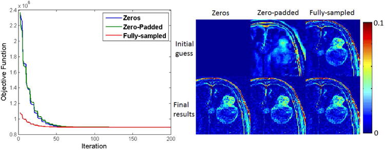
Objective function versus iteration number for three initial TK parameter estimates (left), and cropped portions of these initial and final TK maps (shown is the K^trans map) at a undersampling rate of 20× (right). All initial conditions converged to the same solution. No benefit was observed using a zero-padded k-space relative to a null starting condition.

Figure 3 top shows the phantom results (cropped at the tumor part) of indirect and direct reconstruction of the K^trans and v_p maps at R=1 (fully-sampled data) and R=60 for both direct and indirect method. At R=1, it is shown that the direct method does not introduce additional error by enforcing the Patlak model into the reconstruction. At R=60, the direct method performs better than indirect method for both K^trans and v_p maps, overcoming the large errors and noise introduced by indirect method. Figure 3 bottom shows the rMSE (calculated in tumor boundary ROI) performance across different R. Across all R tested, the direct method outperformed indirect method at high undersampling rates.

Figure 3.

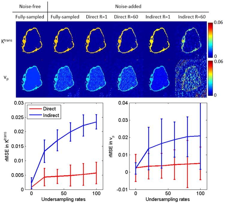
Retrospective evaluation of indirect and direct methods on phantom data. The top row contains ground truth K^trans and v_p maps that are used to generate the phantom, Patlak fitting results from fully-sampled but noise-added data, and R=1 and R=60 reconstruction results for both direct and indirect methods. Realistic noise (SNR=20) were added to the simulated k-space data. The bottom row contains rMSE across undersampling rates for a region of interest containing the entire tumor boundary (761 voxels). The proposed direct reconstruction produced lower mean rMSE at all sampling rates.

Figure 4 shows one representative example of the image results of direct and indirect reconstruction. K^trans and v_p maps of a glioblastoma patient at three different undersampling rates obtained from fully sampled data, the proposed direct reconstruction, and via indirect reconstruction are shown. Across all undersampling rates, the direct method qualitatively, and quantitatively depicted equal or more accurate restoration of TK parameter maps compared to indirect method. At R of 20× or less, the direct and indirect methods had equivalent performance. At higher undersampling rates, the indirect method failed to capture critical tumor signals and tumor shapes in K^trans maps and small vessel information in v_p maps, while the direct method was able to provide accurate restoration. The results with spatial wavelet constraints (only 100× shown here) provide improved noise performance and image quality. It is also worth noting that the indirect method tends to underestimate K^trans values, while the direct method overcomes this underestimation. This is better observed in the Bland-Altman plots in Figure 6.

Figure 4.

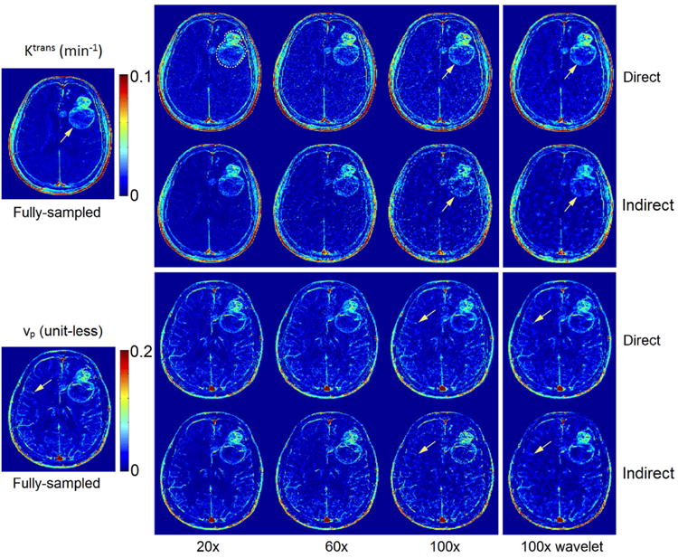
Retrospective evaluation of direct and indirect reconstruction of K^trans and v_p maps. Both reconstructions are shown without spatial wavelet sparsity constraints in the first three columns, and with the sparsity constraint in the last column. By visual inspection, direct reconstruction outperformed indirect results at all undersampling rates. The direct method provided superior delineation of the tumor boundary and other high resolution features in the K^trans maps than did the indirect method. This was particularly true at the highest undersampling rate (see arrows at 100×). For v_p maps, the direct method better preserved small vessel signals (see arrows at 100×) compared to the indirect method. Spatial wavelet constraints, shown on the rightmost column with 100×, provide additional noise suppression.

Figure 6.

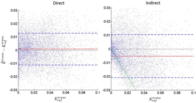
Bland-Altman plots of the difference between estimated K^trans and reference K^trans (from fully-sampled reconstruction) for both direct and indirect method at R=100×. Each dot corresponds to one voxel within the tumor ROI of one of the 13 cases. The indirect reconstruction (right) demonstrated a pattern of underestimating K^trans values, especially for K^trans < 0.02 min^-1 (see green line). This may be a side-effect of the temporal finite difference constraint suppressing small concentration changes. In contrast, the direct reconstruction (left) did not demonstrate any considerable bias patterns, and had a lower variance.

Figure 5 shows tumor ROI K^trans rMSE plots for both methods for a range of undersampling rates, and all 13 data sets that we used for retrospective evaluation. The error bars show the variance introduced by varying the initial angle of the sampling patterns. The direct method outperformed the indirect method for all the cases at high undersampling factors (>80×). The cases are ordered (left to right) by decreasing performance of direct reconstruction compared to indirect reconstruction. More detailed analysis can be found in Table 1.

Figure 5.

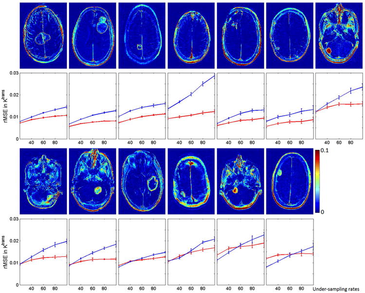
Tumor ROI (fully-sampled) and rMSE plot for direct and indirect reconstruction results across different R (20× to 100×) and 13 data sets for K^trans values. The error bar indicate the mean and variance of the rMSE for each R where 10 different realization of sampling patterns were used. The direct method outperformed the indirect method in most cases, especially at R>60×. The variance for the two methods are comparable.

Table 1.

Patient demographic information and the rMSE performance (mean and standard diviations) of K^trans and v_p for direct and indirect methods at R=60×. The patient order is sorted as the direct reconstruction performance degraded (same as figure 6). At a significance level of p<0.05 (for individual case, p<0.0038 after Bonferroni correction), the direct method performed better than the indirect method for all the cases, with the cut-off undersampling rates varying between 20× to 80×. The p-value for the cut-off undersampling rate is shown in the last column.

No.	Age/Sex	Diagnosis	Indirect 60×		Direct 60×		Significant different at R>	p-value
			Ktrans rMSE (×10e-4)	vp rMSE (×10e-4)	Ktrans rMSE (×10e-4)	vp rMSE (×10e-4)
1	75M	Meningioma	117±2.1	237±4.1	96±2.0	219±6.3	20×	3.72×10-7
2	74M	Glioblastoma	107±2.0	250±6.2	76±1.2	188±4.2	20×	6.3×10-9
3	73M	Glioma	120±3.8	305±9.5	99±3.2	258±9.4	20×	2.55×10-8
4	69F	Meningioma	178±4.5	313±8.3	103±3.4	201±6.2	20×	4.1×10-10
5	77M	Glioma	90±4.7	191±8.3	82±5.2	178±7.4	20×	6.86×10-6
6	39F	Meningioma	114±5.0	192±10.5	83±4.7	191±8.2	20×	1.75×10-6
7	54F	Glioma	167±5.1	358±14.5	156±4.4	376±17.3	40×	2.41×10-6
8	44F	Meningioma	155±6.4	327±13.1	123±5.6	281±14.3	40×	6.57×10-6
9	60M	Glioblastoma	130±5.0	306±10.2	113±5.5	261±10.1	40×	9.73×10-7
10	38F	Glioma	134±5.4	457±6.8	129±5.3	424±6.2	60×	7.42×10-5
11	63M	Meningioma	135±5.4	361±10.6	136±6.9	352±22.0	80×	1.25×10-6
12	73F	Glioma	171±6.1	436±18.2	171±6.6	433±16.5	80×	3.84×10-4
13	79F	Glioma	133±9.5	318±13.0	137±4.7	316±12.2	80×	1.31×10-4

Figure 6 shows the Bland-Altman plots of direct and indirect methods for the K^trans values combining the ROIs of all the 13 cases. The indirect method tended to suppress K^trans values smaller than 0.02 min^-1, and tended to underestimate values larger than 0.02 min^-1. This is similar to a soft-thresholding operation, and is illustrated by the green line in Figure 6. This may be a side-effect of the temporal finite difference constrained reconstruction that suppresses small temporal changes of concentration. Such a trend was not observed in the direct reconstruction, suggesting that tighter integration the TK model is able to identify and restore low K^trans values.

Table 1 lists the patient demographic information, and the performance of direct and indirect methods at R=60×, evaluated by rMSE for both K^trans and v_p maps. The mean and standard deviation of rMSE are listed. The order of presentation in this table matches the order of Figure 6. The normality assumptions are met by Shapiro-Wilk test, and only 4 out of 56 cases (13 patients, 5 undersampling rates) reject the null hypothesis of composite normality assumption at significance level of 0.05. A two-tailed paired STUDENT's t-test was performed between the two methods based on rMSE of K^trans, and the last two columns show the smallest R where the direct method started to statistically significantly outperform the indirect method (p<0.0038 after Bonferroni correction), and the corresponding p-value. The direct method was consistently better than indirect method across multiple data sets at high undersampling rates, and the difference was statistically significant at R>20× for 6 cases, R>40× for 3 cases, R>60× for 1 case, and R>80× for 3 cases.

Figure 7 illustrates direct reconstruction of K^trans and v_p in two representative prospectively undersampled whole-brain DCE data sets. Panning videos TK maps for all 4 cases are provided in supporting materials. The whole-brain high-resolution TK maps enable visualization of the tumor on any arbitrary reformatted plane, providing a complete depiction of the pathological information, and evaluation of narrow enhancing margin and small lesions. The reconstruction time was approximately 10 hours. This pilot study demonstrates the feasibility of applying direct TK parameter reconstruction to whole-brain DCE-MRI.

Figure 7.

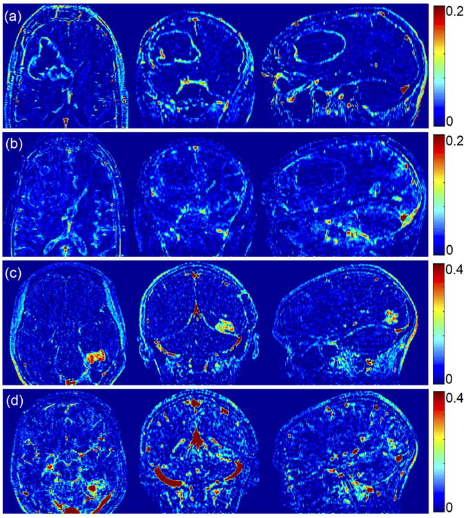
Direct reconstruction of K^trans ((a), (c)) and v_p ((b), (d)) maps from 2 representative prospectively undersampled data. Although lacking gold standard for the prospective studies, the direct reconstruction provided reasonable K^trans values and complete depiction of the entire tumor region. Panning-volume videos for all 4 cases are available in supplementary materials.

Discussion

We have presented a novel and potentially powerful TK parameter estimation scheme for DCE-MRI, where the TK parameter maps are directly reconstructed from undersampled (k,t)-space. By integrating the full forward model connecting the TK maps to the (k,t)-space data in the reconstruction, this method is able to provide excellent TK map fidelity at undersampling rates up to 100×. Higher rates were not tested. The forward model contained the analytic TK model along with specification of the AIF, coil sensitivity maps, and pre-contrast T₁, and M₀ maps obtained from pre-scans. The optimization has the flexibility to incorporate additional spatial sparsity constraints on the TK maps, as demonstrated with a spatial wavelet transform. In the retrospective study, this method outperformed an indirect reconstruction using parallel imaging and compressed sensing. We also uniquely demonstrated the use of this method for prospectively undersampled whole-brain DCE data, where whole-brain TK parameter maps can be produced with excellent image quality.

The proposed method is a “parameter-free” reconstruction, when no spatial constraints are applied to the TK maps. We demonstrated that by simply enforcing the TK model during reconstruction, performance is improved relative to a state-of-the-art compressed sensing reconstruction, without the need to select a constraint or to tune associated regularization parameters. It is straightforward to add sparsity constraints to the optimization problem as shown in [Eqn 7]. Such constraints improve the noise performance, but at the expense of tuning regularization parameters. These constraints were found to improve convergence at very high undersampling rates (>50×) where the TK map estimation problem becomes ill-posed.

The prospective study demonstrates that the proposed method can be used to achieve substantially higher spatial resolution and broader spatial coverage DCE-MRI, while maintaining the same temporal resolution and overall scan time. Although not studied in this work, this approach could potentially be used to improve the temporal resolution of DCE-MRI which is known to provide improvements in patient-specific AIF measurement and TK parameter precision (45).

The proposed method estimates the TK maps directly, and rather than reconstructing image time series as an intermediate step. This enables robust parameter estimation and easy-of-use in clinical application. Clinically, intermediate images (typically 50-100 volumes) are not always viewed. The extracted TK maps are of primary interest as they succinctly describe the behavior of the intermediate images. It is worth noting that the proposed method can provide intermediate images using the full forward model described in Figure 1. Figure 8 compares synthesized images from reconstructed TK maps against fully-sampled anatomic images. The synthesized images show close resemblance to the fully-sampled images.

Figure 8.

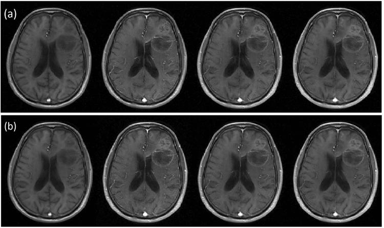
Illustration of intermediate anatomic images from fully-sampled (a), synthesized direct reconstruction at R=30× (b). Images from pre-, peak-, post-, and last- contrast arrival time points are shown from left to right. Anatomic images synthesized from direct estimation of TK parameter maps show similar quality to the fully-sampled and reconstructed anatomic images.

The proposed direct reconstruction scheme requires a-priori definition of the arterial input function (AIF). In this work, we used a population-based AIF, and the time-of-arrival was automatically detected as described in (33). However, other extensions which are blind to the choice of AIF could be explored. For instance, Fluckiger et al. (46) proposed a model-based blind estimation of both AIF and TK parameters from DCE images for fully-sampled data. This approach may be combined with ours to provide joint reconstruction of AIF and TK parameters directly from undersampled data.

This study has a few important limitations. First, we have thus far only demonstrated effectiveness of this approach using the Patlak model. Patlak was chosen because it is widely used and can be linearized and gradients can be readily computed. We also restricted the retrospective study to datasets that fit the Patlak model. It will be important to develop support for more sophisticated models, and utilize data that does not fit the presumed model to fully characterize failure modes. Use of more sophisticated models (e.g. extended Tofts model or 2-compartment exchange model) may fit the data better. Their inclusion will make the reconstruction problem non-linear, and possibly non-convex. Gradient descent algorithms may not be applicable, as they require analytic solution for the first derivative of CA(r,t) with respect to each TK parameter in the model (step 1 for Patlak model in Figure 1). Dikaois et al. (47) recently demonstrated the use of a Bayesian formulation of direct TK parameter estimation in DCE. The rationale was to use an optimal model for different tissue types. The additional complexity of more sophisticated models will necessitate longer reconstruction time, and convergence will require further investigation, and remains as future work.

A second limitation is that the tight integration of TK modeling in our reconstruction could be sensitive to data inconsistencies, such as patient motion. This is equally true for indirect reconstruction. Prospective motion compensation could be added to the proposed model but the complexities involved and efficacy have not been investigated here.

A third limitation is that the intermediate anatomic images are computed during the reconstruction and thus require a similar amount of memory and computation time as indirect methods. This approach is not currently solving the computational limitation of constrained reconstructions but rather provides a framework for improved image quality.

A fourth limitation is that T₁ and M₀ maps are required in the forward model, and were estimated using a separate multiple flip-angle sequence (DESPOT1) performed immediately prior to the DCE scan. Future work could include joint estimation of the pre-contrast T₁ maps and the TK maps, as suggested by Dickie et al. (48).

We compared the direct method with a state-of-the-art indirect method that utilized a temporal finite difference constraint. Compressed sensing techniques are expected to improve steadily as better constraints are identified (49–51); however, if used for TK parameter estimation, a TK model will be applied to the data and model inconsistencies introduced by the intermediate sparsity transforms are likely to propagate into the final parameter maps. Although untested, we hypothesize that our direct estimation method is likely to meet or exceed the image quality of any compressed sensing method.

Our proposed direct reconstruction scheme provides a method for highly accelerated DCE. Extremely high acceleration rates have been demonstrated (up to 100×), enabling full brain DCE with high spatial and temporal resolution. Our method is able to provide a parameter-free reconstruction and so avoids the empirical tuning required in other methods. This technique is easily extendable to DCE-MRI in other body parts such as the breasts, prostate, etc. Future work will include exploration of these additional clinical applications, optimization of data sampling schemes, and integration of more sophisticated TK models.

Conclusion

We have presented a novel and efficient reconstruction scheme to directly estimate TK parameter maps from highly undersampled DCE-MRI data. By comparison with a state-of-the-art indirect compressed sensing method, we demonstrate that the proposed direct approach provides improved TK map fidelity, and enables much higher acceleration. With the prospective study, this method is shown to be clinically feasible and provide high-quality whole-brain TK maps.

Supplementary Material

Supp Video S1

Supporting Document S1: Sampling strategies used in retrospective and prospective under-sampling studies.

Supporting Figure S1: Illustration of the first frame in prospective study: (a) the sampling pattern in ky-kz plane before the contrast injection. (b) the sampling pattern of 30× in a subsequent frame. (c) Inverse Fourier transform of the zero-padded k-space from (a), showing one key slice. (d) Result from averaging all the k-space data points. (e) Result from view-sharing the outer k-space points but keeping the center ¼ points, this is used as first frame in the prospective direct reconstruction.

Supporting Video S1: The sampling pattern changes over time for retrospective under-sampling pattern at 20×, 40×, 60×, 80× and 100×.

Supporting Video S2: The sampling pattern changes over time for Prospective under-sampling pattern at 30×.

Supporting Video S3: The panning volume of the TK parameter maps for prospective study case 0506PJ.

Supporting Video S4: The panning volume of the TK parameter maps for prospective study case 0519JR.

Supporting Video S5: The panning volume of the TK parameter maps for prospective study case 0609SE.

Supporting Video S6: The panning volume of the TK parameter maps for prospective study case 0722SS.

Appendix I: Gradient calculation for the optimization problem

The optimization problem in [Eqn 5] is solved alternatively by a quasi-Newton limited-memory Broyden-Fletcher-Goldfarb-Shanno (l-BFGS) method (36). That is, solving one while keeping the other fixed, as the pseudo codes indicated below:

• Input initial guess K^trans (r)⁽⁰⁾ v_p(r)⁽⁰⁾

• K = 0, while “stopping criteria not met” do {

  $$K^{\mathit{\text{trans}}}{(\mathit{r})}^{(k+1)}=\underset{K^{\mathit{\text{trans}}}(\mathit{r})}{argmin}{\Vert S(\mathit{k},t,c)-y(K^{\mathit{\text{rans}}}(\mathit{r}),v_p{(\mathit{r})}^{(k)})\Vert }_2^2$$ [Eqn A.1]

  $$v_p{(\mathit{r})}^{(k+1)}=\underset{v_p(\mathit{r})}{argmin}{\Vert S(\mathit{k},t,c)-y(K^{\mathit{\text{trans}}}{(\mathit{r})}^{(k+1)},v_p(\mathit{r}))\Vert }_2^2$$ [Eqn A.2]

• K=k=1;}

The gradient of the cost function is evaluated analytically. This can be derived from the model and signal equations. For notational simplicity, the coordinate notations r, k and c are neglected (t is preserved to show the difference in dimension between TK parameter maps and dynamic images). For example, K^trans is for K^trans(r) and S(t) is for S(k,t,c).

In Eqn (A.1), we denote the cost function as:

$$y(K^{\mathit{\text{trans}}},v_p)={\Vert S(t)-f(K^{\mathit{\text{trans}}},v_p)\Vert }_2^2$$

where for one iteration, vp and all other known variables are kept constant, and we focus on deriving the gradient of y w.r.t. K^trans. We use the derivative chain rule:

$$\frac{\partial y}{\partial K^{\mathit{\text{trans}}}}=\frac{\partial \mathit{\text{CA}}(t)}{\partial K^{\mathit{\text{trans}}}}\frac{\partial s(t)}{\partial \mathit{\text{CA}}(t)}\frac{\partial y}{\partial s(t)}$$

where,

$$\begin{array}{c}\frac{\partial y}{\partial s(t)}=C^H{F_u}^H[k_u(t)-f(K^{\mathit{\text{trans}}},v_p)]\hfill \\ \frac{\partial s(t)}{\partial \mathit{\text{CA}}(t)}=r_1{M}_{0}sin\alpha \frac{\mathit{\text{TR}}\cdot e^{-\mathit{\text{TR}}\cdot R_1(t)}\cdot (1-e^{-\mathit{\text{TR}}\cdot R_1(t)}cos\alpha )-(1-e^{-\mathit{\text{TR}}\cdot R_1(t)})\cdot \mathit{\text{TR}}\cdot e^{-\mathit{\text{TR}}\cdot R_1(t)}cos\alpha }{{(1-e^{-\mathit{\text{TR}}\cdot R_1(t)}cos\alpha )}^2}\hfill \\ \frac{\partial \mathit{\text{CA}}(t)}{\partial K^{\mathit{\text{trans}}}}=\sum _{t=0}^{t=t_L}[\underset{0}{\overset{t}{\int }}{C}_p(\tau )d\tau ]\hfill \end{array}$$

Sparsity-based constraints can be optionally applied to the TK maps as shown in [Eqn 6]. In this study, we demonstrate the use of wavelet transform, and we denote the wavelet constrained part as y₁=‖ψx‖₁. For the evaluation of y₁, the l₁ norm is relaxed as in Ref (13):

$$\frac{\partial y_1(K^{\mathit{\text{trans}}})}{\partial K^{\mathit{\text{trans}}}}={\lambda }_1{\psi }^H{W}^{-1}\psi K^{\mathit{\text{trans}}}$$

And the i^th diagonal element of W is calculated as:

$$(W_i=\sqrt{{(\psi K^{\mathit{\text{trans}}})}_i^{\ast }\cdot {(\psi K^{\mathit{\text{trans}}})}_i+\mu )}$$

where μ is a small relaxation parameter.

The gradient for [Eqn A.2] is very similar:

$$\frac{\partial y}{\partial v_p}=\frac{\partial \mathit{\text{CA}}(t)}{\partial v_p}\frac{\partial s(t)}{\partial \mathit{\text{CA}}(t)}\frac{\partial y}{\partial s(t)}$$

where all other parts are the same as above except:

$$\frac{\partial \mathit{\text{CA}}(t)}{\partial v_p}=C_p(t)$$

References

- 1.Larsson HB, Stubgaard M, Frederiksen JL, Jensen M, Henriksen O, Paulson OB. Quantitation of blood-brain barrier defect by magnetic resonance imaging and gadolinium-DTPA in patients with multiple sclerosis and brain tumors. Magn Reson Med. 1990;16:117–131. doi: 10.1002/mrm.1910160111. [DOI] [PubMed] [Google Scholar]
- 2.Law M, Yang S, Babb JS, Knopp EA, Golfinos JG, Zagzag D, Johnson G. Comparison of cerebral blood volume and vascular permeability from dynamic susceptibility contrast-enhanced perfusion MR imaging with glioma grade. Am J Neuroradiol. 2004;25:746–755. [PMC free article] [PubMed] [Google Scholar]
- 3.Yang S, Law M, Zagzag D, Wu HH, Cha S, Golfinos JG, Knopp Ea, Johnson G. Dynamic contrast-enhanced perfusion MR imaging measurements of endothelial permeability: differentiation between atypical and typical meningiomas. AJNR Am J Neuroradiol. 2003;24:1554–9. [PMC free article] [PubMed] [Google Scholar]
- 4.Cramer SP, Simonsen H, Frederiksen JL, Rostrup E, Larsson HBW. Abnormal blood-brain barrier permeability in normal appearing white matter in multiple sclerosis investigated by MRI. NeuroImage Clin. 2014;4:182–189. doi: 10.1016/j.nicl.2013.12.001. [DOI] [PMC free article] [PubMed] [Google Scholar]
- 5.Montagne A, Barnes SR, Law M, et al. Blood-Brain Barrier Breakdown in the Aging Human Report Blood-Brain Barrier Breakdown in the Aging Human Hippocampus. Neuron. 2015;85:296–302. doi: 10.1016/j.neuron.2014.12.032. [DOI] [PMC free article] [PubMed] [Google Scholar]
- 6.O'Connor JPB, Jackson A, Parker GJM, Roberts C, Jayson GC. Dynamic contrast-enhanced MRI in clinical trials of antivascular therapies. Nat Rev Clin Oncol. 2012;9:167–77. doi: 10.1038/nrclinonc.2012.2. [DOI] [PubMed] [Google Scholar]
- 7.Heye AK, Culling RD, Hernández CV, Thrippleton MJ, Wardlaw JM. Assessment of blood – brain barrier disruption using dynamic contrast-enhanced MRI. A systematic review. NeuroImage:Clinical. 2014;6:262–274. doi: 10.1016/j.nicl.2014.09.002. [DOI] [PMC free article] [PubMed] [Google Scholar]
- 8.Tofts PS, Brix G, Buckley DL, et al. Estimating kinetic parameters from dynamic contrast-enhanced T(1)-weighted MRI of a diffusable tracer: standardized quantities and symbols. J Magn Reson Imaging. 1999;10:223–32. doi: 10.1002/(sici)1522-2586(199909)10:3<223::aid-jmri2>3.0.co;2-s. [DOI] [PubMed] [Google Scholar]
- 9.Sourbron SP, Buckley DL. On the scope and interpretation of the Tofts models for DCE-MRI. Magn Reson Med. 2011;66:735–45. doi: 10.1002/mrm.22861. [DOI] [PubMed] [Google Scholar]
- 10.Cramer SP, Larsson HBW. Accurate determination of blood-brain barrier permeability using dynamic contrast-enhanced T1-weighted MRI: a simulation and in vivo study on healthy subjects and multiple sclerosis patients. J Cereb blood flow Metab. 2014;34:1655–1665. doi: 10.1038/jcbfm.2014.126. [DOI] [PMC free article] [PubMed] [Google Scholar]
- 11.Shiroishi MS, Habibi M, Rajderkar D, et al. Perfusion and permeability MR imaging of gliomas. Technol Cancer Res Treat. 2011;10:59–71. doi: 10.7785/tcrt.2012.500180. [DOI] [PubMed] [Google Scholar]
- 12.Sourbron SP, Buckley DL. Classic models for dynamic contrast-enhanced MRI. NMR Biomed. 2013;26:1004–27. doi: 10.1002/nbm.2940. [DOI] [PubMed] [Google Scholar]
- 13.Lustig M, Donoho D, Pauly JM. Sparse MRI: The application of compressed sensing for rapid MR imaging. Magn Reson Med. 2007;58:1182–1195. doi: 10.1002/mrm.21391. [DOI] [PubMed] [Google Scholar]
- 14.Pruessmann KP, Weiger M, Scheidegger MB, Boesiger P. SENSE: sensitivity encoding for fast MRI. Magn Reson Med. 1999;42:952–962. [PubMed] [Google Scholar]
- 15.Uecker M, Lai P, Murphy MJ, Virtue P, Elad M, Pauly JM, Vasanawala SS, Lustig M. ESPIRiT-an eigenvalue approach to autocalibrating parallel MRI: Where SENSE meets GRAPPA. Magn Reson Med. 2014;71:990–1001. doi: 10.1002/mrm.24751. [DOI] [PMC free article] [PubMed] [Google Scholar]
- 16.Lebel RM, Jones J, Ferre JC, Law M, Nayak KS. Highly accelerated dynamic contrast enhanced imaging. Magn Reson Med. 2014;71:635–644. doi: 10.1002/mrm.24710. [DOI] [PubMed] [Google Scholar]
- 17.Guo Y, Lebel RM, Zhu Y, Lingala SG, Shiroishi MS, Law M, Nayak K. High-resolution whole-brain DCE-MRI using constrained reconstruction: Prospective clinical evaluation in brain tumor patients. Med Phys. 2016;43:2013–2023. doi: 10.1118/1.4944736. [DOI] [PMC free article] [PubMed] [Google Scholar]
- 18.Feng L, Grimm R, Block KT, Chandarana H, Kim S, Xu J, Axel L, Sodickson DK, Otazo R. Golden-Angle Radial Sparse Parallel MRI : Combination of Compressed Sensing, Parallel Imaging, and Golden-Angle Radial Sampling for Fast and Flexible Dynamic Volumetric MRI. Magn Reson Med. 2014;72:707–717. doi: 10.1002/mrm.24980. [DOI] [PMC free article] [PubMed] [Google Scholar]
- 19.Chandarana H, Feng L, Ream J, Wang A, Babb JS, Block KT, Sodickson DK, Otazo R. Respiratory Motion-Resolved Compressed Sensing Reconstruction of Free-Breathing Radial Acquisition for Dynamic Liver Magnetic Resonance Imaging. Invest Radiol. 2015;50:749–756. doi: 10.1097/RLI.0000000000000179. [DOI] [PMC free article] [PubMed] [Google Scholar]
- 20.Rosenkrantz AB, Geppert C, Grimm R, et al. Dynamic contrast-enhanced MRI of the prostate with high spatiotemporal resolution using compressed sensing, parallel imaging, and continuous golden-angle radial sampling: Preliminary experience. J Magn Reson Imaging. 2015;41:1365–1373. doi: 10.1002/jmri.24661. [DOI] [PMC free article] [PubMed] [Google Scholar]
- 21.Haldar JP, Hernando D, Liang Z. Super-resolution Reconstruction of MR Image Sequences with Contrast Modeling. IEEE Int Symp Biomed Imaging From Nano to Macro. 2009:266–269. [Google Scholar]
- 22.Ma D, Gulani V, Seiberlich N, Liu K, Sunshine JL, Duerk JL, Griswold Ma. Magnetic resonance fingerprinting. Nature. 2013;495:187–92. doi: 10.1038/nature11971. [DOI] [PMC free article] [PubMed] [Google Scholar]
- 23.Welsh CL, Dibella EVR, Adluru G, Hsu EW. Model-based reconstruction of undersampled diffusion tensor k-space data. Magn Reson Med. 2013;70:429–440. doi: 10.1002/mrm.24486. [DOI] [PMC free article] [PubMed] [Google Scholar]
- 24.Sumpf TJ, Uecker M, Boretius S, Frahm J. Model-based nonlinear inverse reconstruction for T2 mapping using highly undersampled spin-echo MRI. J Magn Reson Imaging. 2011;34:420–8. doi: 10.1002/jmri.22634. [DOI] [PubMed] [Google Scholar]
- 25.Zhao B, Lam F, Liang ZP. Model-based MR parameter mapping with sparsity constraints: Parameter estimation and performance bounds. IEEE Trans Med Imaging. 2014;33:1832–1844. doi: 10.1109/TMI.2014.2322815. [DOI] [PMC free article] [PubMed] [Google Scholar]
- 26.Peng X, Liu X, Zheng H, Liang D. Exploiting parameter sparsity in model-based reconstruction to accelerate proton density and T2 mapping. Med Eng Phys. 2014;36:1428–1435. doi: 10.1016/j.medengphy.2014.06.002. [DOI] [PubMed] [Google Scholar]
- 27.Wang G, Qi J. Direct estimation of kinetic parametric images for dynamic PET. Theranostics. 2013;3:802–815. doi: 10.7150/thno.5130. [DOI] [PMC free article] [PubMed] [Google Scholar]
- 28.Kamasak ME, Bouman Ca, Morris ED, Sauer K. Direct reconstruction of kinetic parameter images from dynamic PET data. IEEE Trans Med Imaging. 2005;24:636–50. doi: 10.1109/TMI.2005.845317. [DOI] [PubMed] [Google Scholar]
- 29.Lin Y, Haldar J, Li Q, Conti P, Leahy R. Sparsity Constrained Mixture Modeling for the Estimation of Kinetic Parameters in Dynamic PET. IEEE Trans Med Imaging. 2013;33:173–185. doi: 10.1109/TMI.2013.2283229. [DOI] [PMC free article] [PubMed] [Google Scholar]
- 30.Felsted BK, Whitaker RT, Schabel M, DiBella EVR. Model-based reconstruction for undersampled dynamic contrast-enhanced MRI. Proc SPIE. 2009;7262:1–10. [Google Scholar]
- 31.Dikaios N, Arridge S, Hamy V, Punwani S, Atkinson D. Direct parametric reconstruction from undersampled (k, t)-space data in dynamic contrast enhanced MRI. Med Image Anal. 2014;18:989–1001. doi: 10.1016/j.media.2014.05.001. [DOI] [PubMed] [Google Scholar]
- 32.Parker GJM, Roberts C, Macdonald A, Buonaccorsi Ga, Cheung S, Buckley DL, Jackson A, Watson Y, Davies K, Jayson GC. Experimentally-derived functional form for a population-averaged high-temporal-resolution arterial input function for dynamic contrast-enhanced MRI. Magn Reson Med. 2006;56:993–1000. doi: 10.1002/mrm.21066. [DOI] [PubMed] [Google Scholar]
- 33.Lebel RM, Guo Y, Zhu Y, Lingala SG, Frayne R, Andersen LB, Easaw J, Nayak KS. The comprehensive contrast-enhanced neuro exam. Proc International Society of Magnetic Resonance in Medicine (ISMRM) 2015:3705. [Google Scholar]
- 34.Deoni SCL, Peters TM, Rutt BK. High-resolution T1 and T2 mapping of the brain in a clinically acceptable time with DESPOT1 and DESPOT2. Magn Reson Med. 2005;53:237–41. doi: 10.1002/mrm.20314. [DOI] [PubMed] [Google Scholar]
- 35.Li KL, Zhu XP, Waterton J, Jackson a. Improved 3D quantitative mapping of blood volume and endothelial permeability in brain tumors. J Magn Reson Imaging. 2000;12:347–57. doi: 10.1002/1522-2586(200008)12:2<347::aid-jmri19>3.0.co;2-7. [DOI] [PubMed] [Google Scholar]
- 36.Liu DC, Nocedal J. On the limited memory BFGS method for large scale optimization. Math Program. 1989;45:503–528. [Google Scholar]
- 37.Guo Y, et al. usc-mrel/DCE_direct_recon: Release 1. Zenodo 2016. doi: http://doi.org/10.5281/zenodo.154058.
- 38.Ramani S, Fessler JA. Parallel MR image reconstruction using augmented Lagrangian methods. IEEE Trans Med Imaging. 2011;30:694–706. doi: 10.1109/TMI.2010.2093536. [DOI] [PMC free article] [PubMed] [Google Scholar]
- 39.Zhu Y, Guo Y, Lingala SG, Barnes S, Lebel RM, Law M, Nayak KS. Proc International Society of Magnetic Resonance in Medicine (ISMRM) 2015. Evaluation of DCE-MRI data sampling, reconstruction and model fitting using digital brain phantom; p. 3070. [Google Scholar]
- 40.Winkelmann S, Schaeffter T, Koehler T, Eggers H, Doessel O. An optimal radial profile order based on the Golden Ratio for time-resolved MRI. IEEE Trans Med Imaging. 2007;26:68–76. doi: 10.1109/TMI.2006.885337. [DOI] [PubMed] [Google Scholar]
- 41.Zhu Y, Guo Y, Lingala SG, Marc Lebel R, Law M, Nayak KS. GOCART: GOlden-angle CArtesian randomized time-resolved 3D MRI. Magn Reson Imaging. 2016;34:940–50. doi: 10.1016/j.mri.2015.12.030. [DOI] [PubMed] [Google Scholar]
- 42.Shellock FG, Kanal E. Guidelines and recommendations for MR imaging safety and patient management. III. Questionnaire for screening patients before MR procedures. J Magn Reson Imaging. 1994;4:749–751. doi: 10.1002/jmri.1880040519. [DOI] [PubMed] [Google Scholar]
- 43.Kanal E, Barkovich AJ, Bell C, et al. ACR guidance document for safe MR practices: 2007. Am J Roentgenol. 2007;188:1447–1474. doi: 10.2214/AJR.06.1616. [DOI] [PubMed] [Google Scholar]
- 44.Stanisz GJ, Henkelman RM. Gd-DTPA relaxivity depends on macromolecular content. Magn Reson Med. 2000;44:665–667. doi: 10.1002/1522-2594(200011)44:5<665::aid-mrm1>3.0.co;2-m. [DOI] [PubMed] [Google Scholar]
- 45.De Naeyer D, De Deene Y, Ceelen WP, Segers P, Verdonck P. Precision analysis of kinetic modelling estimates in dynamic contrast enhanced MRI. MAGMA. 2011;24:51–66. doi: 10.1007/s10334-010-0235-6. [DOI] [PubMed] [Google Scholar]
- 46.Fluckiger JU, Schabel MC, DiBella EVR. Model-based blind estimation of kinetic parameters in Dynamic Contrast Enhanced (DCE)-MRI. Magn Reson Med. 2009;62:1477–1486. doi: 10.1002/mrm.22101. [DOI] [PMC free article] [PubMed] [Google Scholar]
- 47.Dikaios N, Punwani S, Atkinson D. Proc International Society of Magnetic Resonance in Medicine (ISMRM) Direct parametric reconstruction from (k, t)-space data in dynamic contrast enhanced MRI; p. 2015.p. 3706. [Google Scholar]
- 48.Dickie BR, Banerji A, Kershaw LE, Mcpartlin A, Choudhury A, West CM, Rose CJ. Improved accuracy and precision of tracer kinetic parameters by joint fitting to variable flip angle and dynamic contrast enhanced MRI data. Magn Reson Med. 2015;76:1270–1281. doi: 10.1002/mrm.26013. [DOI] [PubMed] [Google Scholar]
- 49.Lingala S, Hu Y, DiBella E, Jacob M. Accelerated Dynamic MRI Exploiting Sparsity and Low-Rank Structure: k-t SLR. IEEE Trans Med Imaging. 2011;30:1042–1054. doi: 10.1109/TMI.2010.2100850. [DOI] [PMC free article] [PubMed] [Google Scholar]
- 50.Hu Y, Lingala SG, Jacob M. A fast majorize-minimize algorithm for the recovery of sparse and low-rank matrices. IEEE Trans Image Process. 2012;21:742–53. doi: 10.1109/TIP.2011.2165552. [DOI] [PubMed] [Google Scholar]
- 51.Miao X, Lingala SG, Guo Y, Jao T, Nayak KS. Accelerated Cardiac Cine Using Locally Low Rank and Total Variation Constraints. Proc International Society of Magnetic Resonance in Medicine (ISMRM) 2015:571. [Google Scholar]
Associated Data
This section collects any data citations, data availability statements, or supplementary materials included in this article.
Supplementary Materials