Efficient 3D Reconstruction in Ultrasound Elastography via a Sparse Iteration based on Markov Random Fields

Abstract

Percutaneous needle-based liver ablation procedures are becoming increasingly common for treatment of small isolated tumors in hepatocellular carcinoma patients who are not candidates for surgery. Rapid three dimensional visualization of liver ablations has potential clinical value because it can enable interventional radiologists to plan and execute needle-based ablation procedures with real time feedback. Ensuring the right volume of tissue is ablated is desirable to avoid recurrence of tumors from residual untreated cancerous cells. Shear wave velocity measurements can be used as a surrogate for tissue stiffness to distinguish stiffer ablated regions from softer untreated tissue. This paper extends the previously reported sheaf reconstruction method to generate complete three dimensional visualizations of shear wave velocities without resorting to an approximate intermediate step of reconstructing transverse C-planes. The noisy data is modeled using a Markov random field, and a computationally tractable reconstruction algorithm that can handle grids with millions of points is developed. Results from simulated ellipsoidal inclusion data show that this algorithm outperforms standard nearest neighbor interpolation by an order of magnitude in mean squared reconstruction error. Results from phantom experiments show that it also provides a higher contrast-to-noise ratio by almost 2 dB and better SNR in the stiff inclusion by over 2 dB compared to nearest neighbor interpolation and has lower computational complexity than linear and spline interpolation.

I. Introduction

Ultrasound elastography is a safe and rapid method for imaging elastic properties of tissues. Following the pioneering work of Ophir et al. [1] that laid the groundwork for signal processing methods for estimating displacements and strain from raw ultrasound echo data (quasi-static ultrasound elastography), research in ultrasound-based tissue elasticity imaging has now enabled the measurement of many different properties such as Young’s modulus [2], shear modulus [3], [4], shear wave velocity (SWV) [5]–[9] and viscoelastic properties [10]. The present paper deals with the problem of reconstruction of three dimensional (3D) visualization of SWVs from data acquired over two dimensional (2D) image planes.

Electrode vibration-based shear wave elastography (EVE) [7], [8] is a type of transient elastography technique which is particularly suited for monitoring percutaneous needle-based ablation procedures. Radiofrequency and microwave ablation have become common clinical procedures in interventional radiology for treating hepatocellular carcinoma [11]. Ablation is typically used for patients who are not candidates for surgical resection and have a fairly localized tumor of diameter less than 5 cm [12].

Ablation uses electromagnetic heating to above 60°C which causes protein denaturation and cell necrosis [13]. As part of the treatment planning stage, patients typically undergo an MRI or CT scan to locate the tumor. B-mode ultrasound is used during the minimally invasive procedure to guide the ablation needle into the tumor, and the procedure is followed by a post-ablation MR or CT scan to ensure that the right volume of cancerous tissue is treated [14]. Ablation planning and monitoring is important because residual untreated cancerous cells may cause the tumor to recur and necessitates additional treatment if seen on post-ablation scans.

B-mode ultrasound does not provide a reliable way to locate the ablation boundary because tissue echogenicity may not be correlated with stiffness [15]. On the other hand, ultrasound shear wave elastography has the potential to provide immediate feedback to clinicians about the extent of an ablation by using the speed of a shear wave as a surrogate for tissue stiffness [16]–[18]. Although it is safer and faster than other imaging modalities that use ionizing radiation, it has the disadvantage of not being able to provide the same level of high resolution 3D reconstructions. Ultrasound elastography is typically used to obtain 2D image reconstructions of tissue stiffness because 1D array probes are still more commonly used in clinical procedures than 2D matrix arrays. Although it may be possible to perform 3D transient elastography using a 2D matrix array transducer [19], [20] the frame rates are too low to track the propagation of a shear wave in a single volume acquisition. Therefore, a method for rapidly reconstructing a 3D visualization from multiple 2D slice acquisitions has clinical value.

The sheaf of ultrasound planes reconstruction (SOUPR) method was presented in [21] for obtaining C-plane (i.e., transverse plane) reconstructions of SWVs. Instead of using an approximate approach of reconstructing individual transverse planes, the present paper proposes a more general method for reconstruction on a full 3D grid while also handling ill-posed situations where the number of grid points may exceed the number of data points. A computationally tractable algorithm that can handle large grid sizes with millions of grid points in 3D is also presented. A standard method for dealing with fast interpolation of scattered data on a grid is through nearest neighbor interpolation [22], and has been previously used for 3D reconstruction of B-mode ultrasound images from 2D slices [23]. The algorithm presented here provides an order of magnitude better mean squared reconstruction error and higher signal-to-noise ratio than nearest neighbor interpolation, as demonstrated through simulations and data acquired from a tissue mimicking (TM) phantom experiment.

II. Theory

A. Markov Random Field Model

A Markov random field (MRF) generalizes the one-dimensional Markov property to higher dimensions. This is useful, for instance, when the random process is a function of spatial co-ordinates instead of time. Let {X₁, X₂, …, X_t, …} be a sequence of discrete valued random variables forming a Markov chain. Then the joint conditional density function of a variable conditioned on the past satisfies the following property:

$$P(X_t|X_1,\dots ,X_{t-1})=P(X_t|X_{t-1}).$$

The same idea can be extended to a “random field” indexed by spatial co-ordinates as follows. Consider an infinite lattice of nodes indexed by triplets −∞ < i, j, k < ∞. The MRF property can be written as:

$$\begin{array}{r}P(X_{i^{\ast },j^{\ast },k^{\ast }}|\{X_{i,j,k}:i\ne i^{\ast },j\ne j^{\ast },k\ne k^{\ast }\})\\ =P(X_{i^{\ast },j^{\ast },k^{\ast }}|\left\{X_{i^{\ast }\pm 1,j^{\ast }\pm 1,k^{\ast }\pm 1}\right\}),\end{array}$$

that is, the value at any given node when conditioned on its immediate neighbors is independent of all other node values. These conditions can be analogously defined using continuous density functions (instead of discrete probability mass functions) for random variables defined on a continuous state space. Also, in practice, it is assumed that the grid size is finite 1 ≤ i ≤ N_y, 1 ≤ j ≤ N_x and 1 ≤ k ≤ N_z where N_x, N_y and N_z respectively denote the number of grid points along the x, y and z dimensions of the 3D volume.

For this paper, a 3D lattice Ising model [24, Ch. 1] is used because the final goal is to reconstruct the measured quantity on a fine grid of points in 3D. An Ising model captures the dependence of values at each grid node as influenced by the values at its immediate neighboring nodes.

A similar idea was used by Gorce et al. [25] to model radiofrequency (RF) ultrasound data for spectral processing. Temporarily ignoring the grid points lying on the boundary, a 6-neighborhood of each node as shown in Fig. 1 is used to define “clique potentials” as follows [26]:

$$\begin{array}{l}V(u_{i,j,k})={(u_{i,j,k}-d_{i,j,k})}^2\\ +\lambda {[\left(\frac{u_{i,j+1,k}+u_{i,j-1,k}-2u_{i,j,k}}{\mathrm{\Delta }{x}^2}\right)}^2\\ +{\left(\frac{u_{i+1,j,k}+u_{i-1,j,k}-2u_{i,j,k}}{\mathrm{\Delta }{y}^2}\right)}^2\\ +{\left(\frac{u_{i,j,k+1}+u_{i,j,k-1}-2u_{i,j,k}}{\mathrm{\Delta }{z}^2}\right)}^2],\end{array}$$ (1)

where d_i,j,k is the value of the data point closest to the node at lattice location (i, j, k) and Δx, Δy, Δz are the grid resolutions along the three axes. The intuition behind using this potential function is as follows. The first term is a data fidelity term that encourages the node values to be close to the values at nearby data points. The next three terms are second order finite differences that approximate the second derivative at each node location to promote smoothness.

Fig. 1.

A 6-neighborhood of grid nodes is used to calculate the clique potential at each grid point using (1). The data point nearest to the central grid point is also used to maintain data fidelity.

Let u denote an N_x N_y N_z × 1 vector consisting of the individual u_{i, j,k} values¹. The “energy function” is defined as the sum of the potentials over all cliques:

$$E(\mathbf{u})={\displaystyle \sum _{\mathbf{i},\mathbf{j},\mathbf{k}}\mathbf{V}({\mathbf{u}}_{\mathbf{i},\mathbf{j},\mathbf{k}})}.$$

By the Hammersley-Clifford theorem, the joint density function for the state u of the MRF can be expressed as [27]:

$$p(\mathbf{u})=\frac{\mathbf{1}}{\mathbf{Z}}\exp (-\mathbf{E}(\mathbf{u}))$$

where Z is a normalization that ensures that p integrates to unity.

B. Iterative Reconstruction Algorithm

The goal of a reconstruction algorithm is to estimate the mode of this distribution, i.e., the value of u which maximizes p(u), or equivalently, minimizes − log p(u) = log Z + E(u). In most situations, it is impossible to calculate Z explicitly because it involves integrating over all possible node values. However, the value of Z is not required for this minimization problem, and it is sufficient to find a minimizer for E(u).

In practice the reconstruction grid size can be quite large. For instance, even in a simple case of a hundred grid points along each of the three axes, the total number of grid points (i.e. the length of the vector u) is 10⁶. A computationally tractable iterative reconstruction approach is shown in Fig. 2. The key idea is to start from an initial guess for the solution and then gradually refine the guess such that the energy function value decreases at each iteration. In order to handle large grid sizes, it is important that the updates should be easy to compute, both in terms of memory storage requirement and computational complexity.

Fig. 2.

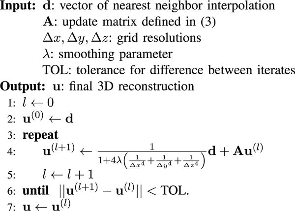
Iterative reconstruction algorithm which starts with an initial guess equal to the nearest neighbor interpolation and refines it using a sparse matrix update equation. The stopping criterion used here examines the progress from one iteration to the next and stops if the norm is smaller than a user defined tolerance. Other stopping criteria (such as a fixing the number of iterations ahead of time) may also be used.

Consider the following greedy algorithm [28, Ch. 17] which updates the value at each node myopically, by using values from the previous iteration for each neighbor. Let u^(l) denote the value of the vector at iteration l, for l ≥ 0. The (i, j, k)th element $u_{i,j,k}^{(l+1)}$ of this vector is obtained by minimizing the potential function in (1) at a fixed coordinate as follows:

$$\begin{array}{l}{u}_{i,j,k}^{(l+1)}=\underset{u}{\arg min}{(u-d_{i,j,k})}^2\\ +\lambda [{\left(\frac{u_{i,j+1,k}^{(l)}+u_{i,j-1,k}^{(l)}-2u}{\mathrm{\Delta }{x}^2}\right)}^2\\ +{\left(\frac{u_{i+1,j,k}^{(l)}+u_{i-1,j,k}^{(l)}-2u}{\mathrm{\Delta }{y}^2}\right)}^2\\ +{\left(\frac{u_{i,j,k+1}^{(l)}+u_{i,j,k-1}^{(l)}-2u}{\mathrm{\Delta }{z}^2}\right)}^2].\end{array}$$

This can be solved in closed form by setting the derivative of the function on the right with respect to u to zero:

$$\begin{array}{l}{u}_{i,j,k}^{(l+1)}=\frac{1}{1+4\lambda \left(\frac{1}{\mathrm{\Delta }{x}^4}+\frac{1}{\mathrm{\Delta }{y}^4}+\frac{1}{\mathrm{\Delta }{z}^4}\right)}[d_{i,j,k}\\ +\frac{2\lambda }{\mathrm{\Delta }{x}^4}(u_{i,j+1,k}^{(l)}+u_{i,j-1,k}^{(l)})\\ +\frac{2\lambda }{\mathrm{\Delta }{y}^4}(u_{i+1,j,k}^{(l)}+u_{i-1,j,k}^{(l)})\\ +\frac{2\lambda }{\mathrm{\Delta }{z}^4}(u_{i,j,k+1}^{(l)}+u_{i,j,k-1}^{(l)})].\end{array}$$

This is similar to the iterated conditional modes (ICM) technique described by Besag [29]. However, note that the update is only a linear combination of the components of u^(l). Therefore, unlike the original ICM algorithm where each pixel is changed individually, the complete vector can be updated in a single step using the following matrix formulation:

$${\mathbf{u}}^{(\mathbf{l}+\mathbf{1})}=\frac{\mathbf{1}}{\mathbf{1}+\mathbf{4}\lambda \left(\frac{\mathbf{1}}{\mathrm{\Delta }{\mathbf{x}}^4}+\frac{\mathbf{1}}{\mathrm{\Delta }{\mathbf{y}}^4}+\frac{\mathbf{1}}{\mathrm{\Delta }{\mathbf{z}}^4}\right)}\mathbf{d}+\mathbf{A}{\mathbf{u}}^{(\mathbf{l})}$$ (2)

where d denotes is a vector of d_i,j_,k values obtained via nearest neighbor interpolation [30], [31]. The matrix A = [a_mn] is defined as:

$$a_{\mathit{mn}}=\{\begin{array}{ll}\frac{2\lambda /\mathrm{\Delta }{x}^4}{1+4\lambda \left(\frac{1}{\mathrm{\Delta }{x}^4}+\frac{1}{\mathrm{\Delta }{y}^4}+\frac{1}{\mathrm{\Delta }{z}^4}\right)}\hfill & \text{if}n=m\pm 1\hfill \\ \frac{2\lambda /\mathrm{\Delta }{y}^4}{1+4\lambda \left(\frac{1}{\mathrm{\Delta }{x}^4}+\frac{1}{\mathrm{\Delta }{y}^4}+\frac{1}{\mathrm{\Delta }{z}^4}\right)}\hfill & \text{if}n=m\pm N_y\hfill \\ \frac{2\lambda /\mathrm{\Delta }{z}^4}{1+4\lambda \left(\frac{1}{\mathrm{\Delta }{x}^4}+\frac{1}{\mathrm{\Delta }{y}^4}+\frac{1}{\mathrm{\Delta }{z}^4}\right)}\hfill & \text{if}n=m\pm N_y{N}_x\hfill \\ 0\hfill & \text{otherwise},\hfill \end{array}$$ (3)

where boundary cases are handled by only considering valid indices 1 ≤ m, n ≤ N_xN_yN_z. It is worth noting the computational complexity of the update equation (2). The matrix A is N_x N_y N_z × N_x N_y N_z and the matrix-vector product would require $O(N_x^2{N}_y^2{N}_z^2)$ multiplications and additions. This can be prohibitive for large grid sizes with millions of grid points. However, note that A is sparse and has at most six non-zero entries per row as seen from (3). Therefore, each element in Au^(l) can be calculated in constant time, resulting in an overall complexity of O(N_x N_y N_z). This is discussed further in Section V.

The following theorem asserts that the sequence of iterates generated in (2) must eventually converge to a limit point. This is proved using a contraction mapping argument in the Appendix.

Theorem

The sequence of iterates {u^(l)} generated by the algorithm in Fig. 2 has a limit point.

Proof: See Appendix. ■

III. Materials and Methods

A. Simulated Ellipsoid Data

The mean squared error (MSE) performance of the 3D reconstruction algorithm was evaluated using simulated ellipsoidal inclusion data with a smooth transition boundary. The SWV value was set to 4 m/s and 1 m/s respectively in the inclusion and the background region. The smooth transition region was modeled using a sigmoid function. The width of this transition region was set to 5 mm following results from [32]. In reality, ablation shapes may be irregular due to presence of blood vessels in the vicinity. An asymmetry is introduced in this ellipsoidal model by setting the SWV in a narrow cylindrical volume equal to 8 m/s.

The “ground truth” SWV values υ(x, y, z) were defined as follows:

$$\upsilon (x,y,z)=\{\begin{array}{l}8,\text{if}{(x-0.25)}^2+{(y-1.2)}^2\le {0.2}^2\hfill \\ 1+3\left(1-\frac{1}{1+e^{-\alpha \left(\frac{x^2}{1^2}+\frac{y^2}{1^2}+\frac{{(z-2.25)}^2}{{1.5}^2}-1\right)}}\right),\text{otherwise}\hfill \end{array}$$ (4)

where the function is evaluated inside −2 ≤ x, y ≤ 2 and 0 ≤ z ≤ 4.5 and the choice of $\alpha =-\frac{1}{0.25}\log \left(\frac{1}{0.99}-1\right)$ captures 98% of the transition region over a width of 5 mm. These numbers were chosen to closely match the dimensions (in cm) of a TM phantom used in Section III-C. The sheaf acquisition pattern was mimicked by sampling this ellipsoid using a cylindrical co-ordinates grid with 4, 6, 12 and 16 image planes. Each image plane was sampled over a 100 × 100 grid, 4 cm wide and 4.5 cm high, i.e., by evaluating (4) inside −2 ≤ x, y ≤ 2 and 0 ≤ z ≤ 4.5. I.i.d Gaussian noise was added to this ground truth data with various noise levels ranging from 5 dB to 20 dB (dB with respect to the inclusion stiffness). A 3D reconstruction was generated using the MRF algorithm listed in Fig. 2 with λ = 0.01, and a grid of size 100×100×100 in a parallelepiped with lateral and elevational dimensions of 4 cm each and depth of 4.5 cm, so that Δx = Δy = 0.04 cm and Δz = 0.045 cm. Mean reconstruction MSE was calculated over 20 independent realizations of the noisy data in a shell of thickness 0.6 cm centered around the ellipsoid boundary. For comparison, the same data was also reconstructed using nearest neighbor interpolation.

B. Finite Element Simulation

An electrode vibration elastography experiment was simulated using a finite element model (FEM) consisting of a stiff inclusion in soft background. The stiffness values were chosen so that the inclusion had a SWV of 4.3 m/s and the surrounding background had a SWV of 1.3 m/s. Details about the FEM can be found in the paper by DeWall et al. [8]. Individual 2D planes in the sheaf were simulated separately due to computational reasons and a limit on the number of nodes. Each image plane was reconstructed using a particle filtering algorithm [33] and registered using the location of the needle as reference.

A 3D reconstruction was generated from the SWV values on registered image planes in the sheaf. The performance of the MRF algorithm was compared with nearest neighbors (NNB) interpolation and linear (LIN) interpolation results. The reconstruction parameters were identical to those used for the simulated ellipsoidal example in Section III-A. The LIN algorithm operates by first calculating a tetrahedralization with all the data points and then uses linear barycentric interpolation in each triangle to estimate the SWV at points on the grid [34].

Various image quality statistics [35], [36] were calculated to compare the reconstruction quality from the MRF algorithm, NNB and LIN interpolation methods. Signal to noise ratio (SNR) is defined as ${\text{SNR}}_{\mathit{inc}}=20{\log }_{10}\frac{{\mu }_{\mathit{inc}}}{{\sigma }_{\mathit{inc}}}$ where the subscript “inc” denotes inclusion. A similar formula is used for the background (“bkg”). Contrast is calculated using $\mathrm{C}=20{\log }_{10}\frac{{\mu }_{\mathit{inc}}}{{\mu }_{\mathit{bkg}}}$ and contrast-to-noise ratio (CNR) using $\text{CNR}=20{\log }_{10}\frac{{\mu }_{\mathit{inc}}-{\mu }_{\mathit{bkg}}}{\sqrt{{\sigma }_{\mathit{inc}}^2+{\sigma }_{\mathit{bkg}}^2}}$. Additionally, MSE with respect to the (known) ground truth SWV values used in the FEA model was also calculated.

C. Tissue Mimicking Phantom Experiment

An oil-in-gelatin based TM phantom [37] consisting of a stiff ellipsoidal inclusion embedded in a softer background material was used for acquiring EVE data. The phantom consisted of a needle firmly glued to the inclusion to simulate the needle in an ablation procedure. A shear wave pulse was set up in the TM phantom by vibrating the needle using a piezoelectric actuator. The actuator was driven by a controller (Physik Instrumente, Germany) that was synchronized with the ultrasound imaging system (Ultrasonix SonixTOUCH, Canada). A half-sinusoid pulse of amplitude 100 microns and width of 20 ms was used to generate the shear wave.

The ultrasound system was operated in research mode which allowed the use of external triggering and a custom scan sequence. A conventional focused transmit acquisition method used to generate B-mode scans does not provide sufficiently high frame rates to track a shear wave. Therefore a phase locked mechanism described in [8] was used to assemble apparent high frame rate RF echo data frames. In this method, multiple pulse vibrations are applied to the needle and only a narrow vertical band of RF data in the image plane is acquired after each vibration. This rests on a reasonable assumption that every pulse has almost identical amplitude and width and there is sufficient delay to allow perturbations from the previous vibration to decay to zero. The 128 element linear array transducer was operated at a center frequency of 5 MHz with the RF data sampled at 40 MHz.

D. Shear Wave Velocity Reconstruction

The method used for reconstructing individual image planes is identical to the one described in [21]. It is assumed that the shear wave pulse travels laterally in the image plane with the needle acting as a line source and particle displacements are purely axial (aligned with the direction of the ultrasound beam lines). A 1D crosscorrelation-based displacement estimation algorithm with axial window length of 2 mm and 1.5 mm overlap is used to determine particle displacements for each pair of consecutive frames. The resulting frame-to-frame displacement movie can be used to localize the shear wave pulse in both space and time. Due to the lateral propagation assumption, the shear wave trajectory can be traced along lines at constant depth radiating away from the needle. The time of peak displacement at each pixel is used as an estimate for the arrival time of the shear wave pulse with sub-frame-number resolution using a 5-point parabolic fit around the peak.

3D reconstructions are generated using the MRF algorithm in Fig. 2. For comparison, nearest neighbors and linear interpolations are also generated and image quality metrics described in Section III-B are calculated. Parallelepiped shaped regions of interest (ROI) of size 5×5×10 mm³ are used to calculate mean and standard deviations of SWVs in the background and inclusion.

IV. RESULTS

A. Simulation Results

As seen in Fig. 3, in all cases the MRF algorithm provides lower MSE than nearest neighbor interpolation by an order of magnitude when reconstructing a simulated ellipsoid with additive Gaussian noise. There is an improvement in MSE performance with increasing number of imaging planes. Due to the smoothness promoting term used in the clique potential function in (1) MRF reconstruction is not as sensitive to noise as NNB.

Fig. 3.

Simulated mean squared error values (in dB) from the ellipsoidal inclusion data with different processing parameters. MSE was calculated with respect to the ground truth model and the average was calculated over 20 independent realizations with added Gaussian noise. MSE was only evaluated in a shell around the ellipsoid boundary. Reconstruction error from a simple nearest neighbor interpolation approach is also shown for comparison.

Image quality metrics for 3D reconstructions generated using the FEM simulation are shown in Tables I and II. The MRF algorithm provides higher SNR, C and CNR values than NNB and LIN algorithms. Mean squared reconstruction errors with respect to the ground truth SWV values are shown in Table III. MRF algorithm provides the lowest MSE of the three algorithms compared.

TABLE I.

Contrast and contrast-to-noise ratios FEM simulation

	Algorithm	4 slices	6 slices	12 slices	16 slices
C	MRF	12.03	11.87	11.70	11.68
	NNB	12.08	11.91	11.77	11.75
	LIN	10.15	10.68	11.06	11.12
CNR	MRF	11.01	9.86	9.49	9.39
	NNB	9.16	8.05	7.74	7.67
	LIN	5.49	7.02	7.76	7.92

Values of contrast (C) and contrast-to-noise ratios (CNR) in dB between the inclusion and the background. (MRF = Markov random field algorithm, NNB = nearest neighbor interpolation, LIN = linear interpolation).

TABLE II.

Signal to noise ratios FEM simulation

ROI	Algorithm	4 slices	6 slices	12 slices	16 slices
bkg	MRF	18.45	18.67	18.75	18.74
	NNB	16.04	16.45	16.23	16.21
	LIN	17.50	16.89	17.33	17.38
inc	MRF	13.60	12.49	12.17	12.07
	NNB	11.75	10.66	10.40	10.34
	LIN	8.78	10.10	10.68	10.82

Signal to noise ratios (SNR) in dB calculated from parallelepiped shaped ROIs in the background and inclusion. The MRF reconstruction has a higher SNR in all cases. (MRF = Markov random field algorithm, NNB = nearest neighbors interpolation, LIN = linear interpolation, bkg = background, inc = inclusion).

TABLE III.

FEM simulation mean squared reconstruction errors

Algorithm	4 slices	6 slices	12 slices	16 slices
MRF	0.24	0.25	0.26	0.26
NNB	0.39	0.41	0.41	0.42
LIN	0.43	0.38	0.35	0.35

Mean squared reconstruction errors are calculated with respect to the ground truth SWV values used in the FEA model. MRF reconstruction gives the lowest MSE in all cases. (MRF = Markov random field algorithm, NNB = nearest neighbors interpolation, LIN = linear interpolation, bkg = background, inc = inclusion).

B. Experimental Results

SWV measurements are averaged over five independent datasets obtained on the same phantom to average out any misregistration errors from manual placement of the transducer probe at different angles [21]. SWV values from the three reconstruction methods are shown in Table IV. Although all methods give similar mean estimates, the MRF algorithm has a lower standard deviation than NNB.

TABLE IV.

Shear wave velocity estimates TM phantom experiment

Algorithm	ROI	4 slices	6 slices	12 slices	16 slices
MRF	bkg	0.80 ± 0.13	0.76 ± 0.11	0.79 ± 0.12	0.79 ± 0.14
	inc	1.53 ± 0.53	1.50 ± 0.50	1.47 ± 0.49	1.48 ± 0.49
NNB	bkg	0.80 ± 0.15	0.76 ± 0.13	0.79 ± 0.14	0.79 ± 0.16
	inc	1.51 ± 0.59	1.49 ± 0.57	1.45 ± 0.57	1.46 ± 0.58
LIN	bkg	0.81 ± 0.13	0.77 ± 0.11	0.79 ± 0.12	0.80 ± 0.13
	inc	1.43 ± 0.51	1.45 ± 0.50	1.45 ± 0.46	1.52 ± 0.60

Mean and standard deviation of shear wave velocities (in m/s) obtained from five independent datasets are shown here. The MRF reconstruction has a lower variance in all cases. (MRF = Markov random field algorithm, NNB = nearest neighbors interpolation, LIN = linear interpolation, bkg = background, inc = inclusion). When measured with a clinical ultrasound scanner (Supersonic Imagine), SWV values for the inclusion and the background were estimated at 1.2 ± 0.03 m/s and 0.9 ± 0.07 m/s respectively.

Table V shows C and CNR values for the three methods with different numbers of image slices used for 3D reconstruction. MRF algorithm provides higher contrast, and also outperforms NNB by 1.96–2.24 dB and LIN interpolation by 0.49–2.13 dB in CNR values, depending on the number of image slices. In the inclusion, SNR values obtained from the MRF reconstruction outperform NNB by over 2 dB and LIN algorithm by 0.54–1.87 dB. This is because the clique potential model in (1) implicitly applies a low pass noise filter by constraining the derivative at each grid point.

TABLE V.

Contrast and contrast-to-noise ratios TM phantom experiment

	Algorithm	4 slices	6 slices	12 slices	16 slices
C	MRF	5.70	5.97	5.43	5.53
	NNB	5.56	5.89	5.30	5.33
	LIN	5.01	5.53	5.30	5.60
CNR	MRF	4.04	4.81	3.67	3.27
	NNB	2.08	2.81	1.45	1.03
	LIN	1.91	3.00	3.18	2.85

Values of contrast (C) and contrast-to-noise ratios (CNR) in dB between the inclusion and the background. All numbers are in dB. The Markov random field algorithm provides slightly better C than nearest neighbor interpolation and also provides higher CNR in the inclusion compared to linear interpolation. (MRF = Markov random field algorithm, NNB = nearest neighbor interpolation, LIN = linear interpolation).

Sample 3D reconstructions from the three methods with 16 image slices are shown in Fig. 4. Reconstructions from NNB interpolation appear blocky, because it fills all the missing grid values with the SWV value from the nearest data point resulting in a “piecewise constant” appearance. Both MRF and LIN algorithms provide smoother reconstructions.

Fig. 4.

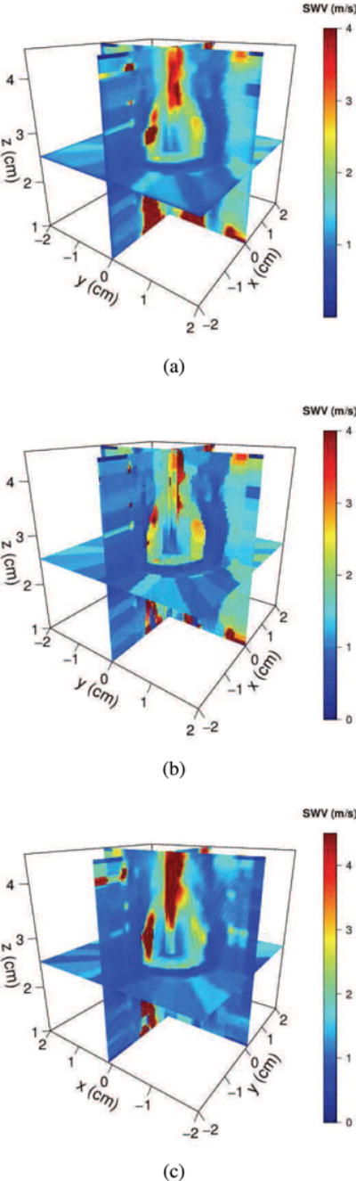
3D reconstructions of SWV values obtained from an electrode vibration elastography tissue-mimicking phantom experiment with 16 slices using the MRF reconstruction algorithm in (a), nearest neighbor interpolation (NNB) in (b) and linear interpolation (LIN) in (c). NNB reconstruction appears more blocky as compared to MRF and has poorer signal-to-noise ratio. Observe that the high velocity artifact to the left of the needle is smaller with MRF compared to LIN. MRF provides a reconstruction on par with the LIN algorithm with an order of magnitude faster reconstruction time and better image quality metrics.

V. Discussion

There is a subtle distinction between the MRF reconstruction algorithm and standard interpolation routines such as NNB and LIN considered in this paper. The MRF method is a function approximation technique as opposed to interpolation. NNB, LIN and other spline fitting algorithms assume that the data points are noiseless and produce reconstructions that respect each data point exactly. However, this may not be a good assumption for 3D SWV reconstruction where point measurements of velocities may be noisy. The MRF algorithm generates a reconstruction that obeys the data points while trying to maintain smoothness; therefore the final reconstruction does not necessarily pass through each data point.

Image quality metrics such as C, CNR and SNR suggest that MRF performs better than LIN for lower number of slices and the disparity decreases as more slices are added. Since MRF does not necessarily force the final fit to pass through the (noisy) data points, it allows greater smoothing to be achieved than LIN, especially with fewer number of image slices. The SNR improvement is greater in the inclusion region where most of the noisy data points and high SWV outliers are present.

As discussed in Section II-B, it is important to consider the algorithmic complexity of these algorithms because it can result in prohibitively long processing times for large grid sizes. NNB has the lowest time complexity among the three algorithms considered in this paper. The MRF algorithm depends on the NNB reconstruction as its initial guess. The proof of convergence in the Appendix suggests that the rate of convergence depends on ‖A‖ which in turn depends on the grid resolution and the smoothing parameter λ. So, provided the NNB result is readily available, the MRF algorithm is almost linear O(N_x N_y N_z) with a constant that depends on grid resolution and the parameter λ in the algorithm in Fig. 2. On the other hand, linear interpolation requires construction of a triangulation from N_d data points in 3D which, in the worst case, can take $O(N_d^2)$ time, and so the algorithm will have a time complexity of $O(N_d^2{N}_x{N}_y{N}_z)$. Depending on the value of N_d, this can cause LIN algorithm to run orders of magnitude slower than the MRF algorithm. For example, the 3D reconstructions shown in Fig. 4 were about 20 times faster with MRF algorithm than linear interpolation.

This paper discussed a specific application of reconstructing a stiff inclusion embedded in a soft background which is usually the case for ablation monitoring. Reflection artifacts can corrupt SWV estimates obtained from time of flight based algorithms. Such artifacts were not visible in pixel displacement profiles for the FEA and phantom data used in this paper because the shear wave originated in the stiffer material. In general, directional filtering [38] will be necessary when generating SWV maps on individual imaging planes before feeding them to the MRF reconstruction algorithm, especially if the shear wave travels through a soft-to-stiff transition boundary. The MRF reconstruction can be applied to visualization of softer inclusions as well, provided the input SWV values are corrected for such artifacts.

The MRF reconstruction algorithm enforces smoothness by penalizing large values of local derivatives. It is important to choose an appropriate value of the penalty parameter λ to avoid over or under-smoothing [21]. This algorithm is naturally suited for handling reconstruction problems where the ground truth does not contain step transitions. It may be necessary to image the volume with sufficient number of imaging planes to capture the boundary irregularities and produce reliable 3D visualizations of highly irregular inclusion shapes. The effect of increasing number of imaging planes on reconstruction is evident in Fig. 3. The location of the irregularity was such that it was not captured by 4, 6 or 8 equi-angular imaging planes. There is a drop in reconstruction MSE when 12 or 16 planes are used. The slight apparent increase in MSE from 12 to 16 planes is a sampling artifact. When using 12 imaging planes, one of the planes happens to coincide precisely with the location of the irregularity; the imaging planes are slightly offset from that location when 16 planes are used.

VI. Conclusion

This paper presented a 3D reconstruction algorithm based on Markov random fields for electrode vibration shear wave elastography. The model-based reconstruction algorithm provides better image quality metrics than standard nearest neighbor interpolation, with improved SNR and CNR and also outperforms linear scattered data interpolation methods in processing speed. Although the results presented in this paper use SWV data, the reconstruction algorithm is quite general and can be applied to other quantitative measurements such as strain, temperature or shear modulus. Moreover, it can also handle ill-posed inverse problems where the grid size is much larger than the number of measurements and the measurements may be scattered at arbitrary locations in a 3D volume.

TABLE VI.

Signal to noise ratios TM phantom experiment

ROI	Algorithm	4 slices	6 slices	12 slices	16 slices
bkg	MRF	22.65	23.14	21.72	17.78
	NNB	21.74	21.87	20.24	16.21
	LIN	23.30	23.83	21.56	18.94
inc	MRF	11.14	11.34	10.72	10.47
	NNB	9.03	9.21	8.51	8.22
	LIN	9.27	9.77	10.18	9.55

Signal to noise ratios (SNR) in dB calculated from parallelepiped shaped ROIs in the background and inclusion. Compared to NNB, the MRF reconstruction has a higher SNR in all cases, and better SNR than LIN in the inclusion. (MRF = Markov random field algorithm, NNB = nearest neighbors interpolation, LIN = linear interpolation, bkg = background, inc = inclusion).

Biographies

Atul Ingle received the B. Tech. in Electronics Engineering from Veermata Jijabai Technological Institute, Mumbai, India in 2009 and the Ph.D. in Electrical Engineering from the University of Wisconsin-Madison, Madison, WI in 2015. He was a visiting R&D engineer at Philips Healthcare Ultrasound in Andover, MA in 2013 and 2014 and is currently a research scientist at Fitbit, Inc. in Boston, MA. His research interests include ultrasound elastography, statistical signal processing for acoustics and ultrasound, and medical image reconstruction algorithms.

Tomy Varghese (S′92-M′95-SM’00) received the B.E. degree in Instrumentation Technology from the University of Mysore, India in 1988, and the M.S. and Ph.D in electrical engineering from the University of Kentucky, Lexington, KY in 1992 and 1995, respectively. From 1988 to 1990 he was employed as an Engineer in Wipro Information Technology Ltd. India. From 1995 to 2000, he was a post-doctoral research associate at the Ultrasonics laboratory, Department of Radiology, University of Texas Medical School, Houston, TX. He is currently a Professor in the Department of Medical Physics at the University of Wisconsin-Madison, Madison, WI. His current research interests include elastography, ultrasound imaging, ultrasonic tissue characterization, detection and estimation theory, statistical pattern recognition and signal and image processing applications in medical imaging. Dr. Varghese is a fellow of the American Institute of Ultrasound in Medicine (AIUM), Senior member of the IEEE, and a member of the American Association of Physicists in Medicine (AAPM) and Eta Kappa Nu.

W.A. Sethares received the Ph.D. degree in electrical engineering from Cornell University, Ithaca, NY. He has worked at the Raytheon Company designing image processing systems and is currently Professor in the Department of Electrical and Computer Engineering at the University of Wisconsin in Madison. Prof. Sethares has held visiting positions at the Australian National University, at the Technical Institute in Gdansk, Poland, at the NASA Ames Research Center in Mountainview CA, and is currently a scientific researcher at the Rijksmuseum in Amsterdam. His research interests include adaptation and learning in signal processing, and decision and estimation in imaging and audio systems. Dr. Sethares is the author of four books, and he holds 7 patents.

Appendix

Proof of Convergence

The iteration in (2) can be represented by a function f: R^N → R^N defined as:

$$f(\mathbf{u})=\frac{\mathbf{1}}{\mathbf{1}+\mathbf{4}\lambda \left(\frac{\mathbf{1}}{\mathrm{\Delta }{\mathbf{x}}^4}+\frac{\mathbf{1}}{\mathrm{\Delta }{\mathbf{y}}^4}+\frac{\mathbf{1}}{\mathrm{\Delta }{\mathbf{z}}^4}\right)}\mathbf{d}+\mathbf{Au}.$$

Let ‖·‖ denote the 2-norm for vectors and the induced spectral 2-norm for matrices. Note that any row of A contains at most six non-zero elements with elements a_mn defined in (3). By the Perron-Frobenius theorem [39], a bound on the largest eigenvalue of A, and hence on ‖A‖ can be obtained as follows:

$$\begin{array}{l}\Vert \mathbf{A}\Vert \le \underset{m}{\max }{\displaystyle \sum _n{a}_{\mathit{mn}}}\\ \le \frac{4\lambda /\mathrm{\Delta }{x}^4}{1+4\lambda \left(\frac{1}{\mathrm{\Delta }{x}^4}+\frac{1}{\mathrm{\Delta }{y}^4}+\frac{1}{\mathrm{\Delta }{z}^4}\right)}\\ +\frac{4\lambda /\mathrm{\Delta }{y}^4}{1+4\lambda \left(\frac{1}{\mathrm{\Delta }{x}^4}+\frac{1}{\mathrm{\Delta }{y}^4}+\frac{1}{\mathrm{\Delta }{z}^4}\right)}\\ +\frac{4\lambda /\mathrm{\Delta }{z}^4}{1+4\lambda \left(\frac{1}{\mathrm{\Delta }{x}^4}+\frac{1}{\mathrm{\Delta }{y}^4}+\frac{1}{\mathrm{\Delta }{z}^4}\right)}\\ =\frac{4{\lambda }^{\prime }}{1+4{\lambda }^{\prime }}\\ <1\end{array}$$

where ${\lambda }^{\prime }=\lambda \left(\frac{1}{\mathrm{\Delta }{x}^4}+\frac{1}{\mathrm{\Delta }{y}^4}+\frac{1}{\mathrm{\Delta }{z}^4}\right)$.

Therefore,

$$\begin{array}{l}\Vert f(\mathbf{u})-\mathbf{f}(\mathbf{v})\Vert =\Vert \mathbf{A}(\mathbf{u}-\mathbf{v})\Vert \\ \le \Vert \mathbf{A}\Vert \Vert \mathbf{u}-\mathbf{v}\Vert \\ <\Vert \mathbf{u}-\mathbf{v}\Vert ,\end{array}$$

where the last step follows from the fact that ‖A‖ < 1. Accordingly, f is a contraction map and by the Banach fixed point theorem [40] the sequence of iterates must converge to a limit point.

References

- 1.Ophir J, Cespedes I, Ponnekanti H, Yazdi Y, Li X. Elastography: a quantitative method for imaging the elasticity of biological tissues. Ultrason Imag. 1991 Apr;13(2):111–134. doi: 10.1177/016173469101300201. [DOI] [PubMed] [Google Scholar]
- 2.Jiang J, Varghese T, Brace CL, Madsen EL, Hall TJ, Bharat S, Hobson MA, Zagzebski JA, Lee FT., Jr Young’s modulus reconstruction for radio-frequency ablation electrode-induced displacement fields: a feasibility study. IEEE Trans Med Imag. 2009 Aug;28(8):1325–1334. doi: 10.1109/TMI.2009.2015355. [DOI] [PMC free article] [PubMed] [Google Scholar]
- 3.Sandrin L, Tanter M, Catheline S, Fink M. Shear modulus imaging with 2-d transient elastography. IEEE Trans Ultrason, Ferroelectr, Freq Control. 2002 Apr;49(4):426–435. doi: 10.1109/58.996560. [DOI] [PubMed] [Google Scholar]
- 4.Palmeri M, Wang M, Dahl J, Frinkley K, Nightingale K. Quantifying hepatic shear modulus in vivo using acoustic radiation force. Ultrasound Med Biol. 2008 Apr;34(4):546–558. doi: 10.1016/j.ultrasmedbio.2007.10.009. [DOI] [PMC free article] [PubMed] [Google Scholar]
- 5.Bercoff J, Tanter M, Fink M. Supersonic shear imaging: a new technique for soft tissue elasticity mapping. IEEE Trans Ultrason, Ferroelectr, Freq Control. 2004 Apr;51(4):396–409. doi: 10.1109/tuffc.2004.1295425. [DOI] [PubMed] [Google Scholar]
- 6.McLaughlin J, Renzi D. Shear wave speed recovery in transient elastography and supersonic imaging using propagating fronts. Inverse Problems. 2006 Mar;22(2):681–706. [Google Scholar]
- 7.Bharat S, Varghese T. Radiofrequency electrode vibration-induced shear wave imaging for tissue modulus estimation: A simulation study. J Acoust Soc Am. 2010 Oct;128(4):1582–1585. doi: 10.1121/1.3466880. [DOI] [PMC free article] [PubMed] [Google Scholar]
- 8.DeWall R, Varghese T, Madsen E. Shear wave velocity imaging using transient electrode perturbation: Phantom and ex vivo validation. IEEE Trans Med Imag. 2011 Mar;30(3):666–678. doi: 10.1109/TMI.2010.2091412. [DOI] [PMC free article] [PubMed] [Google Scholar]
- 9.Song P, Zhao H, Manduca A, Urban M, Greenleaf J, Chen S. Comb-push ultrasound shear elastography (cuse): A novel method for two-dimensional shear elasticity imaging of soft tissues. IEEE Trans Med Imag. 2012 Sep;31(9):1821–1832. doi: 10.1109/TMI.2012.2205586. [DOI] [PMC free article] [PubMed] [Google Scholar]
- 10.Selzo M, Gallippi C. Viscoelastic response (visr) imaging for assessment of viscoelasticity in voigt materials. IEEE Trans Ultrason, Ferroelectr, Freq Control. 2013 Dec;60(12):2488–2500. doi: 10.1109/TUFFC.2013.2848. [DOI] [PMC free article] [PubMed] [Google Scholar]
- 11.Ong SL, Gravante G, Metcalfe MS, Strickland AD, Dennison AR, Lloyd DM. Efficacy and safety of microwave ablation for primary and secondary liver malignancies: a systematic review. European J Gastroenterology & Hepatology. 2009 Jun;21(6):599–605. doi: 10.1097/MEG.0b013e328318ed04. [DOI] [PubMed] [Google Scholar]
- 12.Ferri F. Ferri’s Clinical Advisor 2015. Philadelphia, PA: Elsevier Mosby; 2015. Hepatocellular carcinoma: Treatment. [Google Scholar]
- 13.Knavel EM, Brace CL. Tumor ablation: Common modalities and general practices. Techniques in Vascular and Interventional Radiology. 2013 Dec;16(4):192–200. doi: 10.1053/j.tvir.2013.08.002. [DOI] [PMC free article] [PubMed] [Google Scholar]
- 14.Ziemlewicz TJ, Hinshaw JL, Lubner MG, Brace CL, Alexander ML, Agarwal P, L FT., Jr Percutaneous microwave ablation of hepatocellular carcinoma with a gas-cooled system: Initial clinical results with 107 tumors. Journal of Vascular and Interventional Radiology. 2015 Jan;26(1):62–68. doi: 10.1016/j.jvir.2014.09.012. [DOI] [PMC free article] [PubMed] [Google Scholar]
- 15.Maturen KE, Wasnik AP, Bailey JE, Higgins EG, Rubin JM. Posterior acoustic enhancement in hepatocellular carcinoma. J Ultrasound Med. 2011 Apr;30(4):111–134. doi: 10.7863/jum.2011.30.4.495. [DOI] [PubMed] [Google Scholar]
- 16.DeWall RJ, Varghese T, Brace CL. Visualizing ex vivo radiofrequency and microwave ablation zones using electrode vibration elastography. Med Phy. 2012 Nov;39(11):6692–6700. doi: 10.1118/1.4758061. [DOI] [PMC free article] [PubMed] [Google Scholar]
- 17.Lee SH, Chang JM, Kim WH, Bae MS, Cho N, Yi A, Koo HR, Kim SJ, Kim JY, Moon WK. Differentiation of benign from malignant solid breast masses: comparison of two-dimensional and three-dimensional shear-wave elastography. European Radiol. 2013 Apr;23(4):1015–1026. doi: 10.1007/s00330-012-2686-9. [DOI] [PubMed] [Google Scholar]
- 18.Gennisson JL, Provost J, Deffieux T, Papadacci C, Imbault M, Pernot M, Tanter M. 4-d ultrafast shear-wave imaging. IEEE Trans Ultrason, Ferroelectr, Freq Control. 2015 Jun;62(6):1059–1065. doi: 10.1109/TUFFC.2014.006936. [DOI] [PubMed] [Google Scholar]
- 19.Wang M, Byram B, Palmeri M, Rouze N, Nightingale K. Imaging transverse isotropic properties of muscle by monitoring acoustic radiation force induced shear waves using a 2-d matrix ultrasound array. IEEE Trans Med Imag. 2013 Sep;32(9):1671–1684. doi: 10.1109/TMI.2013.2262948. [DOI] [PMC free article] [PubMed] [Google Scholar]
- 20.Wang M, Byram B, Palmeri M, Rouze N, Nightingale K. On the precision of time-of-flight shear wave speed estimation in homogeneous soft solids: initial results using a matrix array ransducer. IEEE Trans Ultrason, Ferroelectr, Freq Control. 2013 Apr;60(4):758–770. doi: 10.1109/TUFFC.2013.2624. [DOI] [PMC free article] [PubMed] [Google Scholar]
- 21.Ingle A, Varghese T. Three-dimensional sheaf of ultrasound planes reconstruction (soupr) of ablated volumes. IEEE Trans Med Imag. 2014 Aug;33(8):1677–1688. doi: 10.1109/TMI.2014.2321285. [DOI] [PMC free article] [PubMed] [Google Scholar]
- 22.Arya S, Mount DM. Proceedings of the Fourth Annual ACM-SIAM Symposium on Discrete Algorithms. Philadelphia, PA: Society for Industrial and Applied Mathematics; 1993. Approximate nearest neighbor queries in fixed dimensions; pp. 271–280. (ser. SODA ’93). [Google Scholar]
- 23.Blancher J, Léger C, Nguyen LD. Time-varying, 3-d echocardiography using a fast-rotating probe. IEEE Trans Ultrason, Ferroelectr, Freq Control. 2004 May;51(5):634–639. [PubMed] [Google Scholar]
- 24.Kindermann R, Snell JL. Markov Random Fields and Their Applications. Vol. 1 Providence, RI: American Mathematical Society; 1980. The ising model. (ser Contemporary Mathematics). [Google Scholar]
- 25.Gorce J-M, Friboulet D, Dydenko I, D’hooge J, Bijnens B, Magnin I. Processing radio frequency ultrasound images: a robust method for local spectral features estimation by a spatially constrained parametric approach. IEEE Trans Ultrason, Ferroelectr, Freq Control. 2002 Dec;49(12):1704–1719. doi: 10.1109/tuffc.2002.1159848. [DOI] [PubMed] [Google Scholar]
- 26.Geman S, Geman D. Stochastic relaxation, gibbs distributions, and the bayesian restoration of images. IEEE Trans Pattern Anal Mach Intell. 1984 Nov;(6):721–741. doi: 10.1109/tpami.1984.4767596. [DOI] [PubMed] [Google Scholar]
- 27.Grimmett GR. A theorem about random fields. Bull London Math Soc. 1973;5(1):81–84. [Google Scholar]
- 28.Cormen TH, Stein C, Rivest RL, Leiserson CE. Introduction to Algorithms. 3rd. Cambridge, MA: MIT Press; 2001. [Google Scholar]
- 29.Besag J. On the statistical analysis of dirty pictures. J Royal Stat Soc Series B. 1986;48(3):259–302. [Google Scholar]
- 30.Bentley JL. Multidimensional binary search trees used for associative searching. Commun ACM. 1975 Sep;18(9):509–517. [Google Scholar]
- 31.Arya S, Mount DM, Netanyahu NS, Silverman R, Wu AY. An optimal algorithm for approximate nearest neighbor searching fixed dimensions. J of the ACM. 1998 Nov;45(6):891–923. [Google Scholar]
- 32.DeWall RJ, Varghese T, Brace C. Quantifying local stiffness variations in radiofrequency ablations with dynamic indentation. IEEE Trans Biomed Eng. 2012 Mar;59(3):728–735. doi: 10.1109/TBME.2011.2178848. [DOI] [PMC free article] [PubMed] [Google Scholar]
- 33.Ingle A, Ma C, Varghese T. Ultrasonic tracking of shear waves using a particle filter. Med Phy. 2015 Nov;42(11):6711–6724. doi: 10.1118/1.4934372. [DOI] [PMC free article] [PubMed] [Google Scholar]
- 34.Barber C, Dobkin D, Huhdanpaa H. The quickhull algorithm for convex hulls. ACM Trans Math Software. 1996 Dec;22(4):469–483. [Google Scholar]
- 35.Varghese T, Ophir J. A theoretical framework for performance characterization of elastography: the strain filter. IEEE Trans Ultrason, Ferroelectr, Freq Control. 1997 Jan;44(1):164–172. doi: 10.1109/58.585212. [DOI] [PubMed] [Google Scholar]
- 36.Varghese T, Ophir J. An analysis of elastographic contrast-to-noise ratio. Ultrasound in Med Biol. 1998 Jul;24(6):915–924. doi: 10.1016/s0301-5629(98)00047-7. [DOI] [PubMed] [Google Scholar]
- 37.Madsen EL, Hobson MA, Shi H, Varghese T, Frank GR. Tissue-mimicking agar/gelatin materials for use in heterogeneous elastography phantoms. Phys Med Biol. 2005 Dec;50(23):55–97. doi: 10.1088/0031-9155/50/23/013. [DOI] [PMC free article] [PubMed] [Google Scholar]
- 38.Song P, Manduca A, Zhao H, Urban M, Greenleaf J, Chen S. Fast shear compounding using robust 2-d shear wave speed calculation and multi-directional filtering. Ultrasound in Med Biol. 2014 Jun;40(6):1343–1355. doi: 10.1016/j.ultrasmedbio.2013.12.026. [DOI] [PMC free article] [PubMed] [Google Scholar]
- 39.Meyer CD. Matrix Analysis and Applied Linear Algebra. Philadelphia, PA: Society for Industrial and Applied Mathematics; 2000. Perron-frobenius theory. [Google Scholar]
- 40.Rudin W. Principles of Mathematical Analysis. 3rd. New York: McGraw-Hill Book Co; 1976. Functions of several variables: The contraction principle; pp. 220–221. ch. 9. [Google Scholar]