Quantifying the influence of global warming on unprecedented extreme climate events

Significance

Extreme climate events have increased in many regions. Efforts to test the influence of global warming on individual events have also increased, raising the possibility of operational, real-time, single-event attribution. We apply four attribution metrics to four climate variables at each available point on a global grid. We find that historical global warming has increased the severity and probability of the hottest monthly and daily events at more than 80% of the observed area and has increased the probability of the driest and wettest events at approximately half of the observed area. Our results suggest that scientifically durable operational attribution is possible but they also highlight the importance of carefully diagnosing and testing the physical causes of individual events.

Abstract

Efforts to understand the influence of historical global warming on individual extreme climate events have increased over the past decade. However, despite substantial progress, events that are unprecedented in the local observational record remain a persistent challenge. Leveraging observations and a large climate model ensemble, we quantify uncertainty in the influence of global warming on the severity and probability of the historically hottest month, hottest day, driest year, and wettest 5-d period for different areas of the globe. We find that historical warming has increased the severity and probability of the hottest month and hottest day of the year at >80% of the available observational area. Our framework also suggests that the historical climate forcing has increased the probability of the driest year and wettest 5-d period at 57% and 41% of the observed area, respectively, although we note important caveats. For the most protracted hot and dry events, the strongest and most widespread contributions of anthropogenic climate forcing occur in the tropics, including increases in probability of at least a factor of 4 for the hottest month and at least a factor of 2 for the driest year. We also demonstrate the ability of our framework to systematically evaluate the role of dynamic and thermodynamic factors such as atmospheric circulation patterns and atmospheric water vapor, and find extremely high statistical confidence that anthropogenic forcing increased the probability of record-low Arctic sea ice extent.

The last decade has witnessed increasing interest in possible connections between historical global warming and individual extreme climate events (1–9). This interest is grounded in both scientific and practical motivations. First, extremes underlie many of the most acute stresses on natural and human systems (10, 11). Understanding the influence of historical warming on extremes is therefore critical for detecting climate change impacts (12, 13). Second, trends in the frequency and/or intensity of extremes have already been detected (10, 11), implying increasing probability of events that are unprecedented in the observed record. Third, continued global warming is likely to cause widespread emergence of unprecedented events in the future (e.g., refs. 10 and 14).

Effective management of climate-related risks therefore requires robust quantification of the probability of extremes in the current and future climate (10). For example, quantification of risk and liability (8, 15), and design of resilient infrastructure and resource management systems (16), must account for both historical nonstationarity and the likelihood of future changes. Similarly, the United Nations mechanisms for climate change compensation, adaptation, and preparation create a practical need to quantify the contribution of historical emissions to individual extreme events (e.g., ref. 17). Finally, connections between historical warming and individual events have become an explicit motivation for decision makers and the public (e.g., ref. 5).

Although the tails of climate distributions have been analyzed for many years (e.g., ref. 18), quantifying the contribution of historical warming to unprecedented events presents an imposing scientific challenge at the nexus of climate dynamics and statistical analysis (5). First, although some local observations are centuries old, much of the climate system is observed only sparsely, and only for the past few decades (19–21). As a result, observational samples are small relative to the magnitude of the most extreme events (20), creating substantial uncertainty in the probability (22, 23). Second, the historical increase in greenhouse forcing has already altered global climate dynamics (e.g., refs. 2, 10, and 20). The probability of some kinds of extremes has thus been affected both by overlaying a trend on the background variability and by changes in the physical processes that create rare events (22, 24–26). However, because climate forcing has increased over the historical period, the observational sample in the present forcing is even smaller than in the full observational record. As a result, distinguishing a change in probability between the earlier and later periods poses a challenge that cannot be readily overcome solely through observational analysis (e.g., refs. 27 and 28), or with the relatively small climate model ensembles conventionally analyzed in efforts such as the Intergovernmental Panel on Climate Change (23).

Given these challenges, a number of approaches to “single-event attribution” have been developed (2–5, 7, 8, 29). These approaches use observations and/or climate models to quantify the influence of historical global warming on the probability and/or severity of individual events (e.g., refs. 6, 22, and 30–38). Each method has its own advantages and assumptions (5). One challenge is that different approaches sometimes yield different attribution statements, either because of differences in how “attribution” is defined, differences in the statistical assumptions or implementation, or differences in which aspect of the event is analyzed (5).

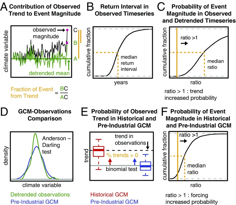
Some methods have matured to the point that “rapid” analyses are now being undertaken (e.g., ref. 39), creating a pathway to operationalize single-event attribution (5, 40). Approaches to evaluate operational attribution are also emerging, including using multiple methods to analyze a single event (38), and using a single method to analyze multiple events (41). In the current study, we analyze multiple types of events using multiple attribution metrics at all available points on a global grid (Fig. 1; Materials and Methods). Our design is philosophically akin to the “precomputed” approach of ref. 40 and the global climate model (GCM)-based analysis of ref. 42. However, we compare multiple attribution metrics, quantify the most extreme event in the observations, and constrain both observational and climate model analyses by the statistical characteristics of the observational record. By extending methods developed for individual localized events to a generalized, global context, our framework provides a systematic evaluation based on observational availability, climate model skill, and the validity of the underlying statistical assumptions.

Fig. 1.

Idealized examples of the primary metrics targeted by our attribution analysis. (A) The contribution of the observed trend to the event magnitude. (B) The uncertainty in the event return interval in the original time series. (C) The uncertainty in the contribution of the observed trend to the event probability. (D) Comparison of the observed interannual variability with the interannual variability simulated by the climate model. (E) The probability of the observed trend in the Historical Climate Model Simulations. (F) The uncertainty in the contribution of the historical forcing to the event probability.

We analyze four variables that test both punctuated and prolonged extremes: the hottest month, hottest day, driest year, and wettest 5-d period. In addition, given the importance of both dynamic and thermodynamic effects (2, 3, 9, 25, 43), we demonstrate the potential to systematically evaluate the occurrence of physical “ingredients” that contribute to individual events.

Results and Discussion

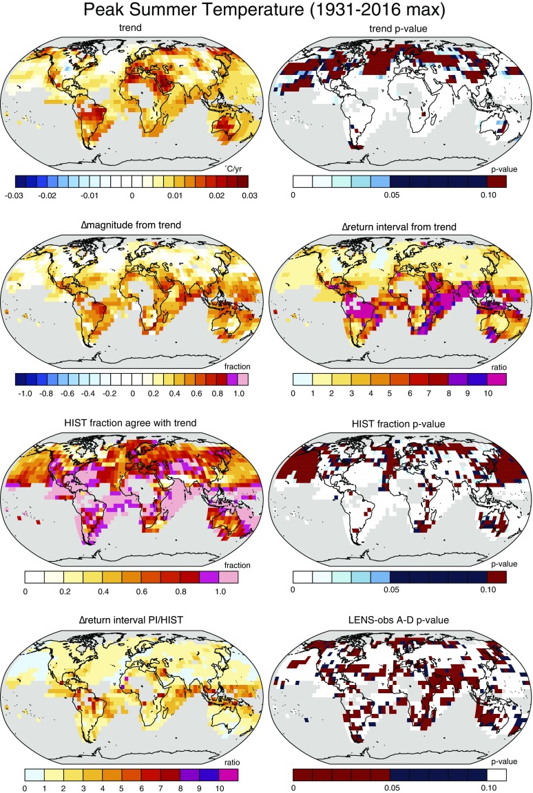
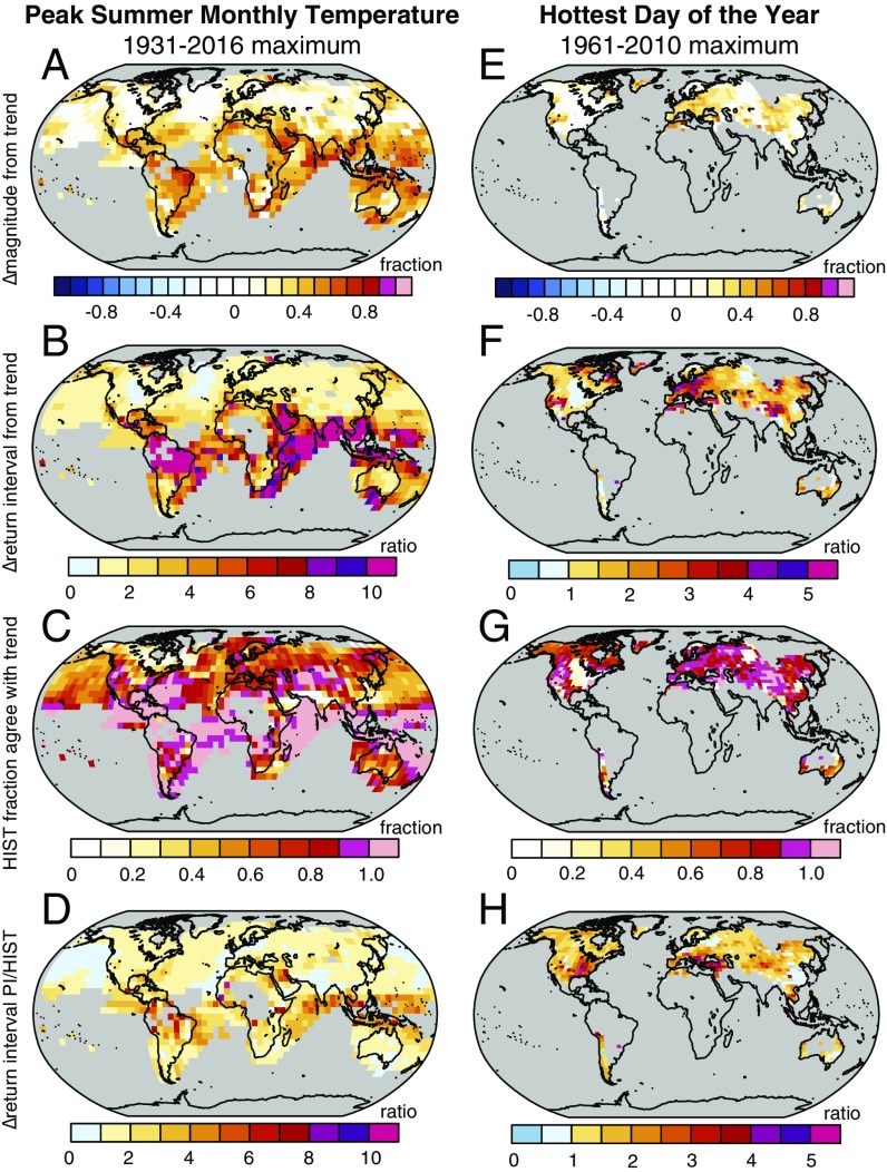
We find that 79% of the observed area exhibits a statistically significant trend in peak summer monthly temperature (Table 1 and Fig. S1). The trend has increased the severity and probability of the maximum peak summer value at 97% of observed area, including over much of the tropics, where the trend has contributed at least 50% of the magnitude and increased the probability by at least a factor of 5 (Fig. 2 A and B). The observed trend is more likely to occur in the Historical Simulations than in a stationary climate over 81% of observed area, with 64% exhibiting high statistical confidence (Table 1 and Fig. 2C). Further, 83% of observed area exhibits higher probability of exceeding the maximum value in the Historical Simulations than in the Pre-Industrial (Table 1), including increases of at least a factor of 4 over large areas of the tropics (Fig. 2D).

Table 1.

Summary of extreme event analysis

Event	Obs trend	∆ magnitude from trend		∆ return interval from trend		GCM-Obs comparison*	GCM Historical trends			∆ return interval from forcing
	Trend P < 0.05	∆mag > 0	>0 and trend P < 0.05	Return ratio > 1	>1 and trend P < 0.05	A-D P > 0.05	Trend fraction > 50%	>50% and A-D P > 0.05	Trend fraction P < 0.05†	Return ratio > 1	>1 and A-D P > 0.05
Peak summer monthly temperature	0.79	0.97	0.78	0.97	0.78	0.71	0.81	0.58	0.64	0.83	0.59
Hottest day of the year	0.41	0.82	0.40	0.83	0.40	0.83	0.82	0.69	0.73	0.85	0.70
Annual precipitation	0.36	0.42	0.14	0.42	0.14	0.55	0.54	0.32	0.34	0.57	0.32
Wettest 5-d period of the year	0.18	0.58	0.12	0.59	0.13	0.80	0.63	0.51	0.06	0.41	0.33

Reported value is the area-weighted fraction of available observations (calculated using the median grid point value, as illustrated in Fig. 1). Obs, observations.

^*Comparison of GCM and observations using A-D test.

^†Where >50% of GCM realizations agree with the observed sign of trend, and P value of trend fraction is <0.05.

Fig. S1.

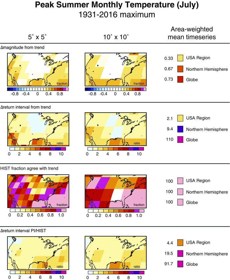
Attribution metrics for the maximum peak summer temperature in the 1931–2016 period. HIST, Historical Climate Model Simulations; PI, Pre-Industrial Control Simulation.

Fig. 2.

Attribution metrics on a global grid for (A−D) the maximum peak summer monthly temperature and (E−H) the maximum hottest day of the year. (A and E) The contribution of the observed trend to the event magnitude. (B and F) The median contribution of the observed trend to the event probability. (C and G) The probability of the observed trend in the Historical Climate Model Simulations. (D and H) The median contribution of the historical forcing to the event probability. HIST, Historical Climate Model Simulations; PI, Pre-Industrial Control Simulation.

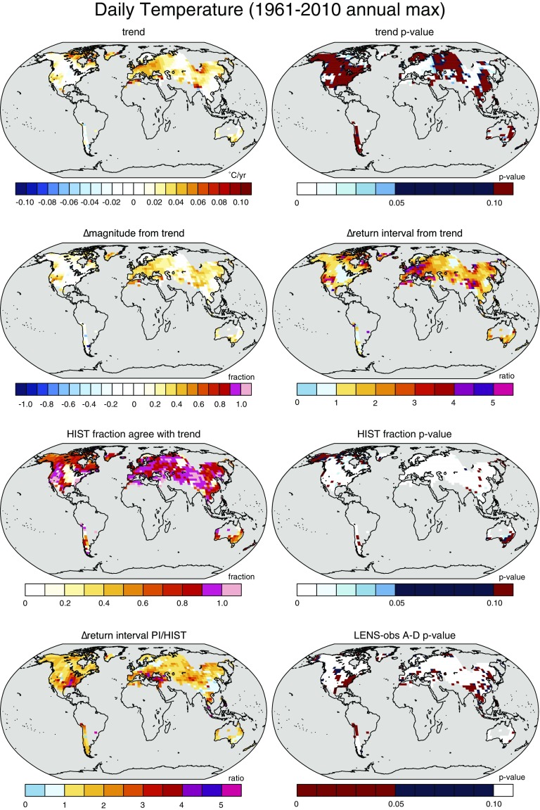
Observations of daily temperature extremes are more sparse, and only 41% of observed area exhibits a statistically significant trend in the hottest daily temperature of the year (Table 1 and Fig. S2). However, the trend has increased the severity and probability of the maximum value at ≥82% of observed area (Table 1), including contributing at least 30% of the magnitude over large areas of Europe and eastern Asia (Fig. 2E), and increasing the probability by at least a factor of 2.5 over most of Europe and parts of western North America and eastern Asia (Fig. 2F). There is high statistical confidence that the observed trend is more likely in the Historical Simulations at 73% of observed area (Table 1), with the most prominent exception being the well-documented “warming hole” over the eastern United States (Fig. 2G). Further, 85% of observed area exhibits a higher probability of exceeding the maximum daily temperature value in the Historical Simulations, including increases of at least a factor of 2 over large areas of North America, Europe, and Asia (Table 1 and Fig. 2H).

Fig. S2.

Attribution metrics for the maximum daily temperature in the 1961–2010 period. HIST, Historical Climate Model Simulations; PI, Pre-Industrial Control Simulation.

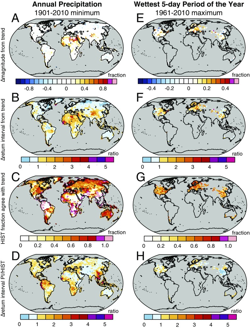
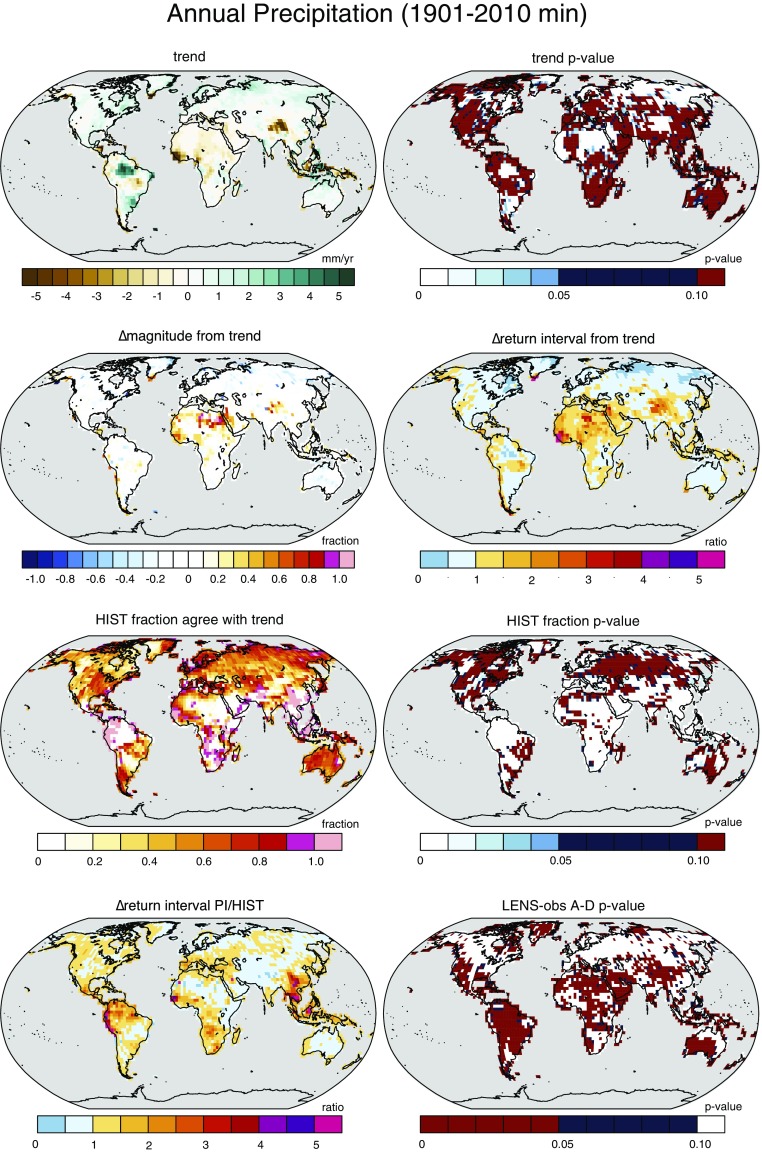
The trend in annual precipitation has increased the severity and probability of the minimum annual precipitation at 42% of observed area (Table 1). Much of this influence of the historical trend is centered in the tropics, where large areas exhibit increased probability of at least a factor of 2 (Fig. 3B). Many of those areas also exhibit a higher probability of the observed annual precipitation trend in the Historical Simulations, including high statistical confidence over areas of tropical South America, tropical Africa, and tropical Southeast Asia (Fig. 3C and Fig. S3). Similarly, 57% of observed area exhibits a higher probability of exceeding the minimum precipitation in the Historical Simulations (Table 1), including at least a factor of 2 over much of tropical North and South America, tropical and southern Africa, and Southeast and East Asia (Fig. 3D).

Fig. 3.

As in Fig. 2, but for (A−D) the minimum annual precipitation and (E−H) the maximum wettest 5-d period of the year. HIST, Historical Climate Model Simulations; PI, Pre-Industrial Control Simulation.

Fig. S3.

Attribution metrics for the minimum annual precipitation in the 1901–2010 period. HIST, Historical Climate Model Simulations; PI, Pre-Industrial Control Simulation.

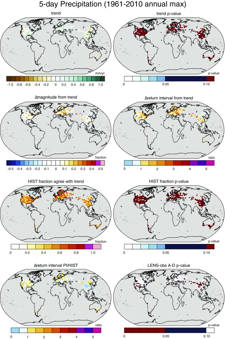
Finally, the historical trend in the wettest 5-d period of the year is statistically significant over only 18% of observed area (Table 1 and Fig. S4). However, the trend has increased the severity and probability of the maximum event at ≥58% of observed area (Table 1), including increases in probability of at least a factor of 1.5 over areas of the United States and Europe (Fig. 3F). In addition, although only 6% of observed area exhibits a significantly higher probability of the observed trend in the Historical Simulations (Table 1 and Fig. 3G), 41% exhibits a higher probability of exceeding the maximum 5-d precipitation value (Table 1 and Fig. 3H).

Fig. S4.

Attribution metrics for the maximum 5-d precipitation in the 1961–2010 period. HIST, Historical Climate Model Simulations; PI, Pre-Industrial Control Simulation.

Quantifying the influence of the historical local trend has important limitations. First, although commonly applied in the literature, the historical trend will not always be accurately represented by a linear model. Second, changes in variance and higher order moments are not accounted for by subtracting a linear trend. Although such changes—and the associated nonlinear effects on event probability—are implicitly included in our comparison of Historical and Pre-Industrial Simulations (Fig. 1F), our analysis of the observed trend (Fig. 1 A and C) effectively assumes that any changes in higher moments did not result from human forcing. Third, because the block bootstrap is implemented to account for relatively short timescale autocorrelation (i.e., subdecadal), it may not account for changes in higher moments that occur over longer timescales. Our framework will therefore benefit from further refinements that explicitly account for nonstationarity in the variance and higher order moments.

Likewise, the strong observational basis of our approach confers both advantages and limitations. First, we emphasize that the observational fractions reported in Table 1 should not be interpreted as fractions of the globe for which the record event can be attributed to anthropogenic forcing. Second, although it is appropriate to compare different types of extremes in areas of overlapping observations (e.g., wet and dry extremes over Europe; Fig. 3 B and F), it is not appropriate to compare the global observational fractions of different extremes, because the observational availability represents very different sampling of the global surface [e.g., although the tropics exhibit the strongest historical temperature emergence (14), the availability of daily temperature and precipitation is heavily biased toward Northern Hemisphere midlatitudes and high latitudes; Fig. S5]. Third, there is uncertainty in the homogeneity of individual instrumental records, and in the spatial aggregation between geographically sparse instruments (19). This uncertainty is generally greater earlier in the observational record, and for shorter-timescale events (19, 44). We have chosen datasets and time periods that balance tradeoffs between longer records and greater spatial coverage, but we note that alternative datasets with more restrictive criteria would further limit the area available for analysis (19, 44). Fourth, our approach does not explicitly account for spatial dependency, which can be large for individual events such as heat waves and severe storms. Although analyzing the atmospheric circulation during such events (e.g., Fig. 4) captures some of this dependence, statistical refinements that explicitly incorporate the spatial dependence structure are also necessary (25). Finally, because the signal-to-noise ratio of climate time series generally increases with spatial scale, the scale at which the analysis is conducted can substantially influence the strength of the attribution results, with the strength increasing from continental to global scale (Fig. S6). This sensitivity suggests that particular care should be taken when analyzing highly localized events.

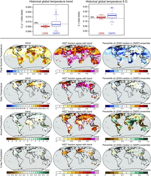
Fig. S5.

(Top) Box-and-whisker plots showing comparison of the global temperature trend (Left) and interannual SD (Right) in gridded observations, the LENS single-model ensemble, and the CMIP5 multimodel ensemble. (Bottom) Maps showing location of the LENS median trend value in the CMIP5 ensemble distribution (Right). For temperature variables, red (blue) colors indicate that the median LENS trend falls in the upper (lower) half of the CMIP5 distribution. For precipitation variables, green (brown) colors indicate that the median LENS trend falls in the upper (lower) half of the CMIP5 distribution. The observed trend (Left) and fraction of the LENS Historical realizations whose trend is of the same sign as the observed trend (Center) are reproduced from Figs. S1−S4 for reference. HIST, Historical Climate Model Simulations; S.D., interannual standard deviation.

Fig. 4.

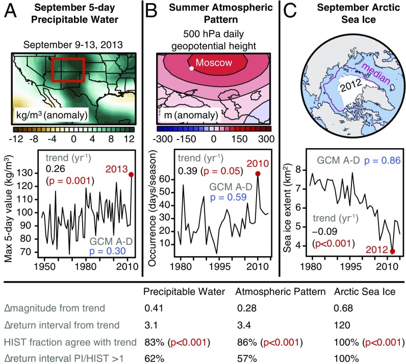
Analysis of climate variables associated with extreme climate events. (A) September 5-d precipitable water associated with the 2013 Colorado floods. (B) Summer 500-hPa geopotential height pattern associated with the 2010 Russia heatwave. (C) September Arctic sea ice extent. HIST, Historical Climate Model Simulations; PI, Pre-Industrial Control Simulation.

Fig. S6.

Quantification of attribution metrics for maximum July temperature at progressively larger spatial scales, including 5° × 5°, 10° × 10°, national, hemispheric, and global. All calculations are made using the grid points that exhibit continuous data availability over the 1931–2016 period (e.g., Fig. 2A). For each spatial scaling, the weighted area average time series is calculated first, and then the attribution metrics are calculated from the weighted area average time series. HIST, Historical Climate Model Simulations; PI, Pre-Industrial Control Simulation.

Our use of a large single-model ensemble similarly presents both advantages and limitations. The strong imprint of internal variability at the local scale creates substantial uncertainty in the influence of anthropogenic climate forcing on individual local trends (e.g., refs. 45 and 46), with even greater uncertainty for extremes than for the long-term mean. Use of a large single-model ensemble (LENS) allows us to objectively quantify the probability that the observed local trend is representative of the forced response, with the null hypothesis being that the local trend arose from climate noise alone (Materials and Methods). However, a major limitation is that the single climate model may not accurately capture the processes that regulate climate variability and/or the response to anthropogenic forcing. At the global scale, all of the LENS realizations simulate less historical warming than both the observations and the majority of the Coupled Model Intercomparison Project Phase 5 (CMIP5) multimodel ensemble (Fig. S5). The fact that LENS captures the observed global temperature variability (Fig. S5) suggests that its cold bias relative to the observed global temperature trend may arise from a lower transient climate sensitivity (47), and/or errors in the prescription of individual forcing factors (e.g., aerosols).

This lower sensitivity could explain why the influence of the trend in observed peak summer temperature is larger than the influence of the historical forcing over most areas (Fig. 2 B vs. D). Indeed, the median LENS peak summer temperature trend falls in the bottom half of the CMIP5 ensemble over most of the observed area (Fig. S5). Interestingly, compared with monthly temperature and annual precipitation, the LENS trends in daily temperature and precipitation are closer to the CMIP5 median over areas of similar data coverage (i.e., North America, Europe, and East Asia). Further, although the global temperature trend is underestimated in LENS, the median LENS annual precipitation trend falls in either the upper or lower CMIP5 quartile over much of the global land area. Together, these grid point comparisons between LENS and CMIP5 suggest that the low global temperature sensitivity in LENS does not result in a universal underestimation of the change in probability of all types of extremes. Disentangling this ambiguity will require large ensembles with additional models, an imposing challenge given that GCMs are not able to simulate the complex conditions that create some types of events (e.g., refs. 21 and 43). Indeed, although LENS agrees with the observations at the majority of observed area (ranging from 55% for annual precipitation to 83% for hottest day of the year; Table 1), large regions of disagreement do occur (e.g., Fig. S3).

We therefore emphasize the importance of understanding the physical processes that give rise to individual events, and of evaluating the ability of climate models to simulate those processes (e.g., refs. 22 and 43). Failure to make these evaluations could lead to erroneous conclusions through either Type I or Type II errors. For example, neither the observed nor simulated trend in extreme precipitation is statistically significant over most grid points (Table 1 and Fig. S4), which could imply that global warming has not substantially influenced such events. However, thermodynamic arguments suggest that global warming should have increased the event probability by increasing atmospheric moisture (2, 48). The 2013 Colorado flooding provides a recent case study (2). We find that the 2013 5-d precipitable water was the highest on record, and that the observed trend and historical forcing contributed substantially to the severity and probability of the 2013 value (Fig. 4A). Likewise, historical analyses show that changes in the frequency of atmospheric patterns have contributed to observed trends in temperature extremes (25). Given the critical role that the atmospheric pressure pattern played in the 2010 Russian heat wave (36), we analyze whether global warming has influenced the frequency of such patterns. We find that the 2010 frequency of daily-scale summertime anticylonic configurations was the largest on record, and that the observed trend and historical forcing contributed substantially to the severity and probability of the 2010 value (Fig. 4B). Although these are just two examples, they highlight the importance of analyzing both the surface expression of the event and the underlying physical causes.

Finally, thermodynamic changes have likely influenced other extremes beyond just temperature and precipitation, including sea level, snowpack, and sea ice (2). Applying our framework to the record-low 2012 September Arctic sea ice extent, we find that the observed trend contributed substantially to the severity and probability of the 2012 value, and that it is “virtually certain” (12) that the historical forcing increased the probability of the event. As with precipitable water and atmospheric pattern occurrence, the climate model ensemble is able to capture the historical variability in September Arctic sea ice (Fig. 4).

Conclusions

We apply four event attribution metrics to a suite of climate variables, including globally gridded temperature and precipitation observations. Our framework is designed to proceed if there is statistical confidence in the fit between the parametric distribution and the observations, if the parametric fit produces a finite solution across the uncertainty distribution, and if the climate model is able to accurately simulate the observed distribution of the variable. Our systematic analysis of global temperature and precipitation data show that these criteria are often met, but also that large areas of the globe can violate these criteria.

The failure of events to meet these criteria arises from at least three conditions. First, unprecedented events result from a complex combination of interacting physical causes. Second, given the rarity of the event, the limitations of the observed record, and the nonstationarity of the climate system, quantifying the probability in the current climate can be highly uncertain. Third, given the complexity of the physical causes, climate models may not accurately simulate the underlying physical processes, or their probability of occurrence.

Our results therefore highlight at least five important priorities for “single event attribution”: (i) understanding the contributions of different physical causes to a particular event, (ii) using formal hypothesis testing to quantify the uncertainty in the probability of both the event and the contributing physical causes, (iii) ensuring accurate assessment of the fidelity of the statistical and physical models to the observational data, (iv) distinguishing changes in the probability of extremes from changes in the mean, and (v) systematically differentiating “absence of evidence” of a causal link from “evidence of absence.”

The ability to robustly quantify the influence of historical global warming on the severity and probability of individual events has important implications for climate adaptation and mitigation efforts, including infrastructure design, resource management practices, disaster risk management systems, quantification of “loss and damage” and legal liability, quantification of the “social cost of carbon,” and “rapid attribution” of individual events. Further, although we have focused on the influence of historical global warming, our framework could be used to quantify the probability of unprecedented events at higher levels of forcing, including those identified in the United Nations Paris Agreement.

Materials and Methods

Observations and Models.

Observations.

Table S1 shows datasets and time periods. We use monthly temperature anomalies from the “NOAAGlobalTemp” gridded dataset (49) to analyze the maximum peak summer temperature (July in the Northern Hemisphere and January in the Southern Hemisphere). We use gridded monthly precipitation from ref. 50 to analyze the minimum annual total precipitation. We use the global gridded observational datasets from ref. 51 to analyze the maximum hottest day of the year and the maximum wettest 5-d period of the year.

Table S1.

Data sources and time periods

Event	Period	Source	Fraction of global grid with observations	Fraction of global area with observations	Fraction of observational area with GCM-Obs A-D P > 0.05	Fraction of observational area with GCM-Obs K-S P > 0.05	LENS runs	LENS period for trends	LENS period for return interval ratios	LENS Historical years	LENS Pre-Industrial years
Peak summer monthly temperature	1931–2016	NCDC (49)	0.45	0.56	0.71	0.84	29	1920–2005	1980–2005	754	1,100
Hottest day of the year	1961–2010	HadEx2 (51)	0.12	0.12	0.83	0.92	29	1956–2005	1980–2005	754	1,100
Annual precipitation	1901–2010	GPCC (50)	0.32	0.35	0.55	0.69	29	1920–2005	1980–2005	754	1,100
Wettest 5-d period of the year	1961–2010	HadEx2 (51)	0.05	0.05	0.80	0.87	29	1956–2005	1980–2005	754	1,100
2013 Boulder, CO, Sept 5-d precipitable water	1948–2013	NCEP/NCAR R-1 (53)	–	–	–	–	29	1920–2005	1980–2005	754	1,799
2010 Russia Jun−Aug anticylonic pattern	1979–2014	NCEP/NCAR R-1 (53)	–	–	–	–	29	1979–2014	1979–2014	1,044	938
2012 Arctic Septemb sea ice	1979–2015	NSIDC (52)	–	–	–	–	34	1979–2015	1980–2005	884	1,100

To explore the potential to quantify the influence of global warming on additional variables beyond temperature and precipitation, we also analyze sea ice data from ref. 52, and geopotential height patterns and precipitable water from ref. 53. The geopotential height patterns are calculated using self-organizing maps as described in ref. 25, with the direct atmospheric “thermal dilation” removed (see ref. 26).

Climate models.

The most prominent climate model experiments are those coordinated by CMIP (e.g., ref. 54). Although CMIP provides simulations from many different climate models, the limited number of realizations means that a relatively small number of simulated years are available from each model in each forcing window, which can create substantial errors in the calculation of return intervals of the most extreme events (23). We therefore analyze the National Center for Atmospheric Research (NCAR) LENS ensemble, which generates a large ensemble (∼30 realizations) of a single model in an individual CMIP5 forcing pathway (e.g., refs. 45 and 55). This approach provides many hundreds of simulated years in a given forcing window (Table S1), captures a much larger range of variability than is available in the observations, and isolates internal climate system variability from model structural uncertainty.

LENS was generated with the NCAR Community Earth System Model run at ∼1° horizontal resolution (55). The ensemble methodology branches multiple GCM simulations from a single CMIP-type transient Historical Simulation. These multiple realizations differ only in slight perturbations in the initial atmospheric conditions in 1920. (We analyze only the branched simulations that were initialized in 1920.) Each ensemble member is then prescribed the transient historical forcing through the end of the CMIP5 historical period (2005), and the Representative Concentration Pathway (RCP8.5) transient forcing after 2005.

We compare the LENS Historical Simulations with the Pre-Industrial Control Simulation (Table S1). Depending on the variable, the observed record may be shorter than the LENS simulations, or only a subset of the observed record may be deemed reliable (e.g., due to reliance on satellite observations). Although the initial period of the RCP8.5 simulations can be used to extend the simulated period past 2005, the lack of other real-world forcings such as volcanic eruptions can affect the fidelity of the simulated climate in the post-2005 period (e.g., ref. 56).

Quantifying the Influence of Global Warming on Individual Events.

We evaluate the locally observed maxima or minima of four widely used extreme temperature and precipitation indicators on a global grid. We calculate four target metrics for each variable (Fig. 1), based on our previously published methods (22, 24, 34, 57). Our choice of these four metrics is motivated by the need to compare different metrics that have been explored in the literature (5), including the contribution of the local historical trend to a given event, and the extent to which historical climate forcing has influenced the probability of a given event. We report results at grid points where the observational dataset is continuous over the analysis period.

The contribution of the observed trend to the magnitude of the event.

We first find the maximum/minimum event in the observed time series at each grid point. We then detrend the observed time series at each grid point, and find the new value of the original event magnitude in the detrended time series (Fig. 1A). We then calculate the contribution of the observed trend to the event magnitude as the difference between the observed event magnitude and the detrended event magnitude, divided by the difference between the observed event magnitude and the mean of the detrended time series (Fig. 1A). We calculate the statistical significance of the observed trend following the approach of ref. 24, which accounts for temporal dependence in the observed time series using the moving block bootstrap.

The contribution of the observed trend to the probability of the event magnitude.

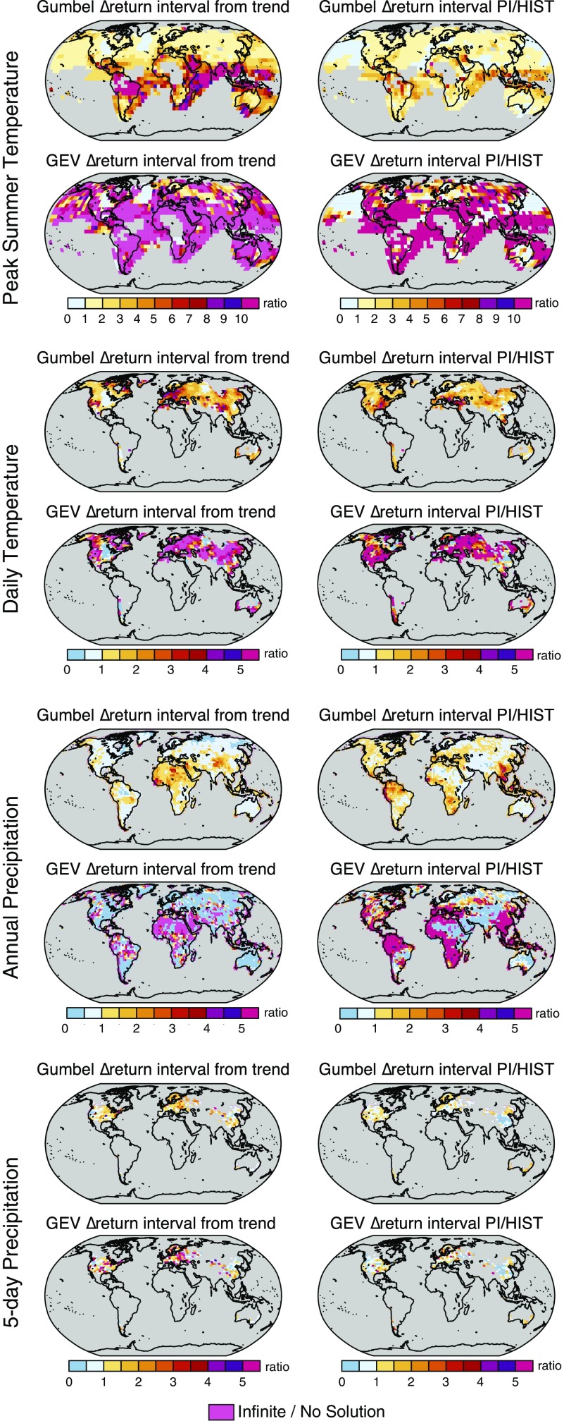
We adapt the approach of refs. 34 and 22 to calculate the ratio of return intervals between the observed and detrended time series. Different authors have used different parametric distributions (e.g., comparison in ref. 34). Here we use the Gumbel variation of the Generalized Extreme Value (GEV) distribution, which, for these variables and these datasets, provides a conservative estimation of the change in probability compared with the more generalized application of the GEV (Fig. S7). However, we note that the Gumbel distribution will not necessarily provide the most conservative estimation in all cases, and therefore care should be taken when selecting the method for calculating the return interval of historically unprecedented events.

Fig. S7.

Comparison of the change in probability calculated using the Gumbel variation of the GEV and the change in probability calculated using the generalized application of the GEV. HIST, Historical Climate Model Simulations; PI, Pre-Industrial Control Simulation.

Because sampling errors tend to be large when data segment lengths are similar to the event return interval (23), the fact that the observational record is limited to several decades is likely to create substantial uncertainty in the calculated return interval of the most extreme events. We therefore follow refs. 34 and 22 in using the moving block bootstrap to account for uncertainty in the fit of the observations to the parametric distribution. As in ref. 24, the length of each subset for the nonparametric block bootstrap—that is, the “block size”—is determined by the number of time steps for which temporal dependence is significant in the time series, based on the partial autocorrelation function of the data. By selecting the block size based on the observed autocorrelation of the data, the moving block bootstrap preserves the observed dependency of the data within—but not among—the blocks. Our application of the moving block bootstap is thereby an approach to ensuring that the statistical assumptions for hypothesis testing hold (i.e., that the block samples in the bootstrap are approximately independent and identically distributed random vectors).

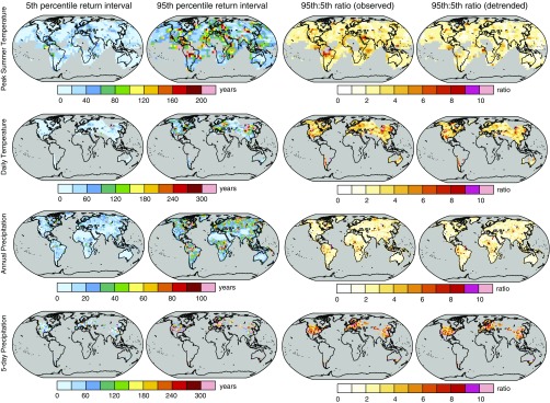
This bootstrapping yields a sample of parametric fits to the observations, which in turn yields a sample of return intervals for the event magnitude in the observed time series (Fig. 1B and Fig. S8). We repeat this process to calculate the sample of return intervals for the event magnitude in the detrended time series. [We find that the return interval uncertainty is very similar between the observed and detrended time series, with peak summer temperature over tropical South America exhibiting the greatest discrepancy (Fig. S8).] Finally, we follow refs. 34 and 22 in calculating the ratio for all possible combinations of return intervals in the observed and detrended time series, yielding an estimate of the uncertainty in the contribution of the observed trend to the event probability (Fig. 1C). We report the median value of the ratio distribution (Fig. 1C) at each grid point.

Fig. S8.

Uncertainty in the return interval of the record event in the observed time series (first three columns) and the detrended time series (fourth column). Note that the maximum (or minimum, respectively) event is removed from the historical data prior to fitting the parametric distribution.

The probability of the observed trend in the historical climate forcing.

We follow the approach of ref. 57 to calculate the probability of the observed trend in the historical forcing (Fig. 1E). We first calculate the fraction of Historical Simulations that exhibit a trend of the same sign as the observed time series. We then evaluate the statistical significance of that fraction using a two-tailed binomial test, where (i) the null hypothesis is that the probability of observing a positive trend is 0.5 and the probability of observing a negative trend is 0.5, and (ii) the P value is calculated as the two-tailed probability that the simulated fraction of trends having the same sign as the observed trend is equal to 0.5. (This method avoids fitting a parametric distribution to the observed or simulated data.)

As in refs. 34 and 22, we evaluate the climate model’s simulation of interannual variability in each climate indicator (Fig. 1D). Previous event attribution studies have made this evaluation using the Kolmogorov−Smirnov test (22, 34, 38). However, we find that the Anderson−Darling (A-D) test, which gives more weight to the tails of the distribution, produces a more restrictive comparison with observations for the four extreme climate variables (Table S1). We therefore use the A-D test. We first correct the mean of the Pre-Industrial Control Simulation to be equal to the mean of the detrended observations. We then use the A-D test to quantify the agreement between the mean-corrected Pre-Industrial Simulation and the detrended observations. We reject the climate model if the A-D test yields a P value less than 0.05, as this suggests that the model output does not come from the same statistical population as the observations.

The probability of the event magnitude in the historical and preindustrial climate forcing.

We follow refs. 34 and 22 in calculating the ratio of return intervals between the Historical and Pre-Industrial GCM Simulations (Fig. 1F). This analysis is similar to that described in The Contribution of the Observed Trend to the Probability of the Event Magnitude for the influence of the historical trend, but performed on the Historical and Pre-Industrial GCM Simulations rather than the observed and detrended time series. The NCAR large ensemble provides >700 y of data in the Historical and Pre-Industrial Simulations (Table S1); in contrast to decadal-scale periods, 1,000-y simulations have been shown to “provide fairly accurate estimates of changes in return levels even for long return periods” (23).

As described in ref. 22, we use the sample of event return intervals in the observations (calculated above) to define the sample of event magnitudes in the climate model simulation: We first define the sample of return intervals in the Pre-Industrial Simulation to be identical to that of the detrended observed time series. We then calculate the sample of event magnitudes in the Pre-Industrial Control Simulation that are associated with that sample of event return intervals. Then, for each of the Pre-Industrial event magnitudes, we calculate the associated event return interval in the Historical Climate Model Simulations. Finally, as described above, we calculate the ratio for all possible combinations of return intervals in the Historical and Pre-Industrial samples, yielding an uncertainty estimate for the contribution of historical forcing to the event probability. We report the median value of the ratio distribution (Fig. 1F) at each grid point.

References

- 1.Trenberth KE. Framing the way to relate climate extremes to climate change. Clim Change. 2012;115:283–290. [Google Scholar]
- 2.Trenberth KE, Fasullo JT, Shepherd TG. Attribution of climate extreme events. Nat Clim Change. 2015;5:725–730. [Google Scholar]
- 3.Shepherd TG. A common framework for approaches to extreme event attribution. Curr Clim Change Reports. 2016;2:28–38. [Google Scholar]
- 4.Stott PA, et al. Attribution of extreme weather and climate-related events. Wiley Interdiscip Rev Clim Change. 2016;7:23–41. doi: 10.1002/wcc.380. [DOI] [PMC free article] [PubMed] [Google Scholar]
- 5.National Academies of Sciences, Engineering, and Medicine . Attribution of Extreme Weather Events in the Context of Climate Change. Natl Acad Press; Washington, DC: 2016. [Google Scholar]
- 6.Stott PA, Stone DA, Allen MR. Human contribution to the European heatwave of 2003. Nature. 2004;432:610–614. doi: 10.1038/nature03089. [DOI] [PubMed] [Google Scholar]
- 7.Coumou D, Rahmstorf S. A decade of weather extremes. Nat Clim Change. 2012;2:491–496. [Google Scholar]
- 8.Allen M, et al. Scientific challenges in the attribution of harm to human influence on climate. Univ Pa Law Rev. 2007;155:1353–1400. [Google Scholar]
- 9.Otto FEL, et al. The attribution question. Nat Clim Change. 2016;6:813–816. [Google Scholar]
- 10.Intergovernmental Panel on Climate Change 2012. Managing the Risks of Extreme Events and Disasters to Advance Climate Change Adaptation eds Field CB, et al. (Cambridge Univ Press, Cambridge, UK)
- 11.Easterling DR, et al. Climate extremes: Observations, modeling, and impacts. Science. 2000;289:2068–2074. doi: 10.1126/science.289.5487.2068. [DOI] [PubMed] [Google Scholar]
- 12.Intergovernmental Panel on Climate Change . Summary for policy makers. In: Field CB, et al., editors. Climate Change 2014: Impacts, Adaptation, and Vulnerability. Contribution of Working Group II to the Fifth Assessment Report of the Intergovernmental Panel on Climate Change. Cambridge Univ Press; Cambridge, UK: 2014. pp. 1–32. [Google Scholar]
- 13.Rosenzweig C, et al. Attributing physical and biological impacts to anthropogenic climate change. Nature. 2008;453:353–357. doi: 10.1038/nature06937. [DOI] [PubMed] [Google Scholar]
- 14.Diffenbaugh NS, Scherer M. Observational and model evidence of global emergence of permanent, unprecedented heat in the 20(th) and 21(st) centuries. Clim Change. 2011;107:615–624. doi: 10.1007/s10584-011-0112-y. [DOI] [PMC free article] [PubMed] [Google Scholar]
- 15.Mills E. Insurance in a climate of change. Science. 2005;309:1040–1044. doi: 10.1126/science.1112121. [DOI] [PubMed] [Google Scholar]
- 16.Milly PCD, et al. Climate change. Stationarity is dead: Whither water management? Science. 2008;319:573–574. doi: 10.1126/science.1151915. [DOI] [PubMed] [Google Scholar]
- 17.Huggel C, Wallimann-Helmer I, Stone D, Cramer W. Reconciling justice and attribution research to advance climate policy. Nat Clim Change. 2016;6:901–908. [Google Scholar]
- 18.Mearns LO, Katz RW, Schneider SH. Extreme high-temperature events: Changes in their probabilities with changes in mean temperature. J Clim Appl Meteorol. 1984;23:1601–1613. [Google Scholar]
- 19.Hartmann DL, et al. In: Climate Change 2013: The Physical Science Basis. Contribution of Working Group I to the Fifth Assessment Report of the Intergovernmental Panel on Climate Change. Stocker TF, et al., editors. Cambridge Univ Press; Cambridge, UK: 2013. pp. 159–254. [Google Scholar]
- 20.Peterson TC, et al. Monitoring and understanding changes in heat waves, cold waves, floods and droughts in the United States: State of knowledge. Bull Am Meteorol Soc. 2013;94:821–834. [Google Scholar]
- 21.Diffenbaugh NS, Trapp RJ, Brooks HE. Does global warming influence tornado activity? Eos Trans AGU. 2008;89:553–554. [Google Scholar]
- 22.Swain DL, et al. The extraordinary California drought of 2013-2014: Character, context, and the role of climate change. Bull Am Meteorol Soc. 2014;95:S3–S7. [Google Scholar]
- 23.Huang WK, Stein ML, McInerney DJ, Moyer EJ. Estimating changes in temperature extremes from millennial-scale climate simulations using generalized extreme value (GEV) distributions. Adv Stat Climatol Meteorol Oceanogr. 2016;2:79–103. [Google Scholar]
- 24.Singh D, Tsiang M, Rajaratnam B, Diffenbaugh NS. Observed changes in extreme wet and dry spells during the South Asian summer monsoon season. Nat Clim Change. 2014;4:456–461. [Google Scholar]
- 25.Horton DE, et al. Contribution of changes in atmospheric circulation patterns to extreme temperature trends. Nature. 2015;522:465–469. doi: 10.1038/nature14550. [DOI] [PubMed] [Google Scholar]
- 26.Swain DL, Horton DE, Singh D, Diffenbaugh NS. Trends in atmospheric patterns conducive to seasonal precipitation and temperature extremes in California. Sci Adv. 2016;2:e1501344. doi: 10.1126/sciadv.1501344. [DOI] [PMC free article] [PubMed] [Google Scholar]
- 27.Lin N, Emanuel K. Grey swan tropical cyclones. Nat Clim Change. 2016;6:106–111. [Google Scholar]
- 28. Stone DA, Paciorek CJ, Prabhat, Pall P, Wehner M (2013) Inferring the anthropogenic contribution to local temperature extremes. Proc Natl Acad Sci USA 110:E1543. [DOI] [PMC free article] [PubMed]
- 29.Easterling DR, Kunkel KE, Wehner MF, Sun L. Detection and attribution of climate extremes in the observed record. Weather Clim Extremes. 2016;11:17–27. [Google Scholar]
- 30.Rahmstorf S, Coumou D. Increase of extreme events in a warming world. Proc Natl Acad Sci USA. 2011;108:17905–17909. doi: 10.1073/pnas.1101766108. [DOI] [PMC free article] [PubMed] [Google Scholar]
- 31.Stone DA, Allen MR. The end-to-end attribution problem: From emissions to impacts. Clim Change. 2005;71:303–318. [Google Scholar]
- 32.Pall P, et al. Anthropogenic greenhouse gas contribution to flood risk in England and Wales in autumn 2000. Nature. 2011;470:382–385. doi: 10.1038/nature09762. [DOI] [PubMed] [Google Scholar]
- 33.Otto FEL, Massey N, Oldenborgh GJ, Jones RG, Allen MR. Reconciling two approaches to attribution of the 2010 Russian heat wave. Geophys Res Lett. 2012;39:L04702. [Google Scholar]
- 34.Singh D, et al. Severe precipitation in Northern India in June 2013: Causes, historical context, and changes in probability. Bull Am Meteorol Soc. 2014;95:S58–S61. [Google Scholar]
- 35.Diffenbaugh NS, Swain DL, Touma D. Anthropogenic warming has increased drought risk in California. Proc Natl Acad Sci USA. 2015;112:3931–3936. doi: 10.1073/pnas.1422385112. [DOI] [PMC free article] [PubMed] [Google Scholar]
- 36.Dole R, et al. Was there a basis for anticipating the 2010 Russian heat wave? Geophys Res Lett. 2011;38:L06702. [Google Scholar]
- 37.Haustein K, et al. Real-time extreme weather event attribution with forecast seasonal SSTs. Environ Res Lett. 2016;11:64006. [Google Scholar]
- 38.Uhe P, et al. Comparison of methods: Attributing the 2014 record European temperatures to human influences. Geophys Res Lett. 2016;43:8685–8693. [Google Scholar]
- 39.van Oldenborgh GJ, et al. Rapid attribution of the May/June 2016 flood-inducing precipitation in France and Germany to climate change. Hydrol Earth Syst Sci Discuss. 2016 doi: 10.5194/hess-2016-308. [DOI] [Google Scholar]
- 40.Christidis N, Stott P, Zwiers F. Fast-track attribution assessments based on pre-computed estimates of changes in the odds of warm extremes. Clim Dyn. 2015;45:1547–1564. [Google Scholar]
- 41.Angélil O, et al. An independent assessment of anthropogenic attribution statements for recent extreme temperature and rainfall events. J Clim. 2017;30:5–16. [Google Scholar]
- 42.Fischer EM, Knutti R. Anthropogenic contribution to global occurrence of heavy-precipitation and high-temperature extremes. Nat Clim Change. 2015;5:560–564. [Google Scholar]
- 43.Mitchell D, et al. Assessing mid-latitude dynamics in extreme event attribution systems. Clim Dyn. August 23, 2016 doi: 10.1007/s00382-016-3308-z. [DOI] [Google Scholar]
- 44.Donat MG, et al. Global land-based datasets for monitoring climatic extremes. Bull Am Meteorol Soc. 2013;94:997–1006. [Google Scholar]
- 45.Deser C, Knutti R, Solomon S, Phillips AS. Communication of the role of natural variability in future North American climate. Nat Clim Change. 2012;2:775–779. [Google Scholar]
- 46.Mankin JS, Viviroli D, Singh D, Hoekstra AY, Diffenbaugh NS. The potential for snow to supply human water demand in the present and future. Environ Res Lett. 2015;10:114016. [Google Scholar]
- 47.Thompson DWJ, Barnes EA, Deser C, Foust WE, Phillips AS. Quantifying the role of internal climate variability in future climate trends. J Clim. 2015;28:6443–6456. [Google Scholar]
- 48.O’Gorman PA. Precipitation extremes under climate change. Curr Clim Change Rep. 2015;1:49–59. doi: 10.1007/s40641-015-0009-3. [DOI] [PMC free article] [PubMed] [Google Scholar]
- 49.Vose RS, et al. NOAA’s merged land-ocean surface temperature analysis. Bull Am Meteorol Soc. 2012;93:1677–1685. [Google Scholar]
- 50.Schneider U, et al. GPCC’s new land surface precipitation climatology based on quality-controlled in situ data and its role in quantifying the global water cycle. Theor Appl Climatol. 2014;115:15–40. [Google Scholar]
- 51.Sillmann J, Kharin VV, Zhang X, Zwiers FW, Bronaugh D. Climate extremes indices in the CMIP5 multimodel ensemble: Part 1. Model evaluation in the present climate. J Geophys Res Atmos. 2013;118:1716–1733. [Google Scholar]
- 52.Cavalieri DJ, Parkinson CL, Gloersen P, Zwally HJ. 2015, c1996. Data from “Sea ice concentrations from Nimbus-7 SMMR and DMSP SSM/I-SSMIS passive microwave data, version 1.” NASA National Snow and Ice Data Center Distributed Active Archive Center. dx.doi.org/10.5067/8GQ8LZQVL0VL.
- 53.Kalnay E, et al. The NCEP/NCAR 40-year reanalysis project. Bull Am Meteorol Soc. 1996;77:437–471. [Google Scholar]
- 54.Taylor KE, Stouffer RJ, Meehl GA. An overview of CMIP5 and the experiment design. Bull Am Meteorol Soc. 2012;93:485–498. [Google Scholar]
- 55.Kay JE, et al. The Community Earth System Model (CESM) Large Ensemble Project: A community resource for studying climate change in the presence of internal climate variability. Bull Am Meteorol Soc. 2015;96:1333–1349. [Google Scholar]
- 56.Santer BD, et al. Volcanic contribution to decadal changes in tropospheric temperature. Nat Geosci. 2014;7:185–189. [Google Scholar]
- 57.Singh D, et al. Recent amplification of the North American winter temperature dipole. J Geophys Res Atmos. 2016;121:9911–9928. doi: 10.1002/2016JD025116. [DOI] [PMC free article] [PubMed] [Google Scholar]