Constraining the instantaneous aerosol influence on cloud albedo

Significance

Uncertainties in the strength of aerosol–cloud interactions drive the current uncertainty in the anthropogenic forcing of the climate. Previous studies have highlighted shortcomings in using satellite data for determining the forcing, which underestimate the strength of the aerosol forcing. This work demonstrates that the component of the radiative forcing from aerosol–cloud interactions due to the instantaneous effect on cloud reflectivity (RFaci) can be calculated to within 20%, using only present-day observations of the variability of aerosol and cloud properties, provided the anthropogenic component of the aerosol is known. The model results are combined with satellite data to provide an improved observations-based estimate of the RFaci, paving the way for more accurate estimates of the aerosol influence on climate.

Abstract

Much of the uncertainty in estimates of the anthropogenic forcing of climate change comes from uncertainties in the instantaneous effect of aerosols on cloud albedo, known as the Twomey effect or the radiative forcing from aerosol–cloud interactions (RFaci), a component of the total or effective radiative forcing. Because aerosols serving as cloud condensation nuclei can have a strong influence on the cloud droplet number concentration (N_d), previous studies have used the sensitivity of the N_d to aerosol properties as a constraint on the strength of the RFaci. However, recent studies have suggested that relationships between aerosol and cloud properties in the present-day climate may not be suitable for determining the sensitivity of the N_d to anthropogenic aerosol perturbations. Using an ensemble of global aerosol–climate models, this study demonstrates how joint histograms between N_d and aerosol properties can account for many of the issues raised by previous studies. It shows that if the anthropogenic contribution to the aerosol is known, the RFaci can be diagnosed to within 20% of its actual value. The accuracy of different aerosol proxies for diagnosing the RFaci is investigated, confirming that using the aerosol optical depth significantly underestimates the strength of the aerosol–cloud interactions in satellite data.

The radiative forcing due to anthropogenic aerosols is the most uncertain component of the anthropogenic radiative forcing (1), with the interaction between aerosols and clouds generating much of this uncertainty. As cloud droplets form on aerosol particles, changes in the aerosol number concentration can change the cloud droplet number concentration (N_d), generating an instantaneous radiative forcing by increasing the cloud brightness, known as the Twomey effect (2) or radiative forcing from aerosol–cloud interactions (RFaci) (1) (referring only to liquid clouds in this work). Together with other changes in cloud properties due to changes in N_d (e.g., ref. 3), the RFaci is a component of the total or effective radiative forcing (ERFaci).

Due to the sparse nature of preindustrial (PI) observations of cloud properties, the influence of aerosols on cloud properties is often inferred from observations of the present-day spatiotemporal variability of aerosol and cloud properties (e.g., refs. 4–7). Although much of the variation between aerosol and cloud properties can be attributed to variations of meteorological factors (e.g., refs. 8 and 9), the sensitivity of N_d to aerosol optical depth (AOD) is thought to be largely independent of these factors. It is therefore often used in observational estimates of the strength of aerosol–cloud interactions (7, 10, 11). This sensitivity (5) has been shown to be a useful “emergent constraint” on the strength of the ERFaci in general circulation models (12), providing a method to calculate the change in N_d from the PI to the present day (PD), when combined with an estimate of the corresponding anthropogenic change in AOD (such as ref. 13). Two main assumptions are made in this process: that the AOD is a suitable proxy of the cloud condensation nuclei (CCN) concentration at the cloud base and that the relationships between aerosol and the N_d in the PD (determined by spatiotemporal variability) are indicative of the actual sensitivity of cloud properties to aerosol perturbations.

Recent work has called both of these assumptions into question. Observational (14) and model-based (15) studies have shown a disconnect between AOD and CCN. Because the AOD is a column-integrated measurement, it does not provide vertical information about the location of the aerosol. It also lacks information about the composition of the particles and is weighted preferentially toward larger particles (4), missing information about smaller aerosol particles that are often emitted from anthropogenic activities (16).

Second, it has been shown that the PD AOD–N_d relationship may not be representative of the true strength of the interaction between aerosols and cloud properties due to the differing PI and PD aerosol environments (17). Additionally, it has been shown (18) that in many global aerosol–climate models the PD sensitivity of N_d to CCN variations (the slope of the linear regression between N_d and CCN concentrations) is in many cases not representative of the sensitivity of N_d to the anthropogenic perturbation of CCN (the PD–PI change in N_d divided by the corresponding change in CCN evaluated from climate simulations). This suggests that it would be challenging to constrain the magnitude of the RFaci using only PD observations of the sensitivity of N_d to aerosol variations.

In this work, techniques are presented to address these challenges. To account for nonlinearity in the aerosol–N_d relationship and the differing PI and PD aerosol environments, normalized joint histograms are used to characterize the relationship (following ref. 11). A variety of different global aerosol–climate models that contributed to the AeroCom intercomparison (18, 19) are used to investigate the utility of different aerosol proxies for diagnosing the anthropogenic change in cloud-top N_d. Together with joint histograms, this work investigates how accurately the RFaci could be diagnosed under ideal conditions, using PD relationships between aerosol and cloud properties.

Results

Aerosol–${\text{𝑵}}_{\text{𝒅}}$ Relationships.

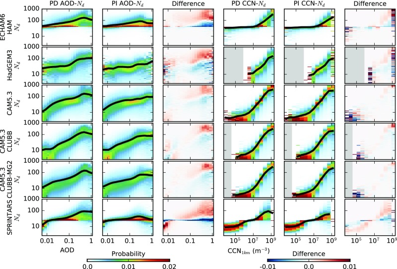
Two-dimensional (“joint”) histograms of N_d and aerosol properties are used in this work to account for the influence of nonlinearities in the relationship (11). Each column of the joint histogram is normalized so that it sums to 1, such that it becomes an array of conditional probabilities. For example, the top left histogram in Fig. 1 shows the probability of finding a specific N_d, given that a certain AOD has been observed.

Fig. 1.

Joint histograms between aerosol properties (AOD and CCN_1km, respectively, x axis) and cloud-top N_d (y axis) for each of the general circulation models (GCMs) used in this study. The first and second columns show the AOD-N_d joint histograms for the PD and the PI simulations, respectively. The histograms are normalized so each column sums to 1, such that the histograms show the probability of observing a specific cloud-top N_d, given a certain AOD (or CCN_1km). The black line shows the mean N_d at each AOD and gray regions indicate missing data. The third column shows the difference between the PD and the PI relationships. The second set of three columns are the same as the first three but use CCN_1km at 0.3% supersaturation instead of AOD as the independent variable.

Joint histograms of cloud-top N_d versus an aerosol proxy for a selection of models from the AeroCom intercomparison (18, 19) (gridded to 2.5° by 2.5°) are shown in Fig. 1. Although there is a general increase in cloud-top N_d with increasing AOD (Fig. 1, first and second columns), the nature of this increase varies significantly among the models. Some of the models (the CAM5 variants) show a strong increase in N_d at lower AOD, followed by a saturation at higher AOD, where the N_d only weakly increases with increasing AOD. Others show a weak AOD–N_d relationship at low AOD, followed by a stronger relationship as the AOD increases (ECHAM6-HAM and SPRINTARS). The enforced lower bound to the N_d apparent in some simulations may be responsible for the lower sensitivity of N_d to AOD ($\frac{d{N}_d}{dln(A)}$) at low AODs in these models (12), although low sensitivities at low AOD have also been observed in satellite data (11).

All of the models show some difference in the AOD–N_d relationship between the PD and the PI (Fig. 1, third column), mostly with higher N_ds for a given AOD in the PD simulation compared with the PI. It is stronger at high AODs, suggesting that this effect is due to the different composition of aerosols in the PD compared with the PI. When the atmosphere is clean (low AOD), the aerosol composition is similar in the PI and the PD simulations. However, high-AOD conditions occur mainly in dusty regions in the PI simulation (where the aerosol is a poor CCN), but in the PD simulation these high-AOD conditions are often the result of anthropogenic pollution (which on average is a much better CCN).

The situation is very different when using CCN at 1-km altitude and 0.3% supersaturation (CCN_1km) instead of the AOD as the parameter representing the aerosol (Fig. 1, fourth column). The CCN_1km–N_d relationships are still mostly nonlinear, although there is less variation between the models than for the AOD–N_d joint histograms. Importantly, the PD and PI CCN_1km–N_d relationships are very similar, showing much smaller differences in the joint histograms than are evident for the AOD–N_d relationship (Fig. 1, sixth column). At lower supersaturations (0.1%) the CCN is weighted toward larger particles and the PD and PI relationships are not as close (Fig. S1). However, the PD global CCN_1km–N_d joint histogram is a reasonable indicator of the PI relationship, as long as there is enough data at low CCN concentrations to properly create a joint histogram.

Fig. S1.

(A–C) As Fig. 3, but using CCN at 0.1% supersaturation. The AI and AOD columns remain the same.

It is also clear that the nonlinearity of these relationships will influence any calculations made using a linear regression, where the sensitivity would otherwise depend on the prevailing aerosol environment (17). By normalizing the joint histograms by the aerosol occurrence, this dependence is removed and with the appropriate choice of aerosol proxy (such as CCN_1km) the PD spatiotemporal variability is a good approximation of the PI variation and thus the actual sensitivity of clouds to aerosol perturbations.

Diagnosing $𝚫{\text{𝑵}}_{\text{𝒅}}$.

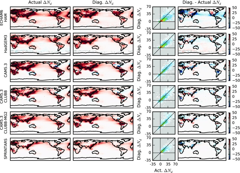
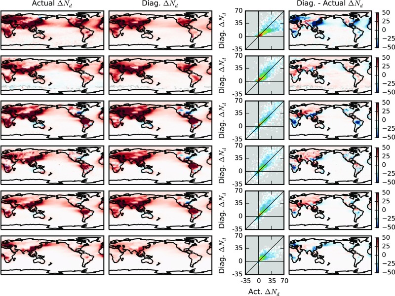
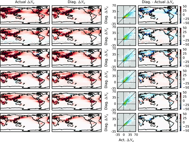
Using regional joint histograms (15° by 15° regions), similar to those from Fig. 1, and probability histograms for CCN_1km from the PI and PD simulations, a prediction for the geographic distribution of $\mathrm{\Delta }{N}_d$ is constructed in Fig. 2. The “actual” $\mathrm{\Delta }{N}_d$ for each model (the difference in N_d between the PD and PI simulations) is shown in the first column of Fig. 2. Both the PI and PD simulations are nudged to the same horizontal winds, such that the “actual” $\mathrm{\Delta }{N}_d$ is due to the difference in aerosol emissions. The $\mathrm{\Delta }{N}_d$ diagnosed using the PD CCN_1km-N_d joint histogram and the PD–PI CCN_1km change (Eq. 1) is shown in the second column.

Fig. 2.

Using joint histograms of CCN_1km versus N_d from 15° by 15° regions to diagnose $\mathrm{\Delta }{N}_d$ (Hist CCN regional). For each model used, the first column shows the annual-mean “actual” $\mathrm{\Delta }{N}_d$ (the N_d difference between the PI and PD simulations). The second shows $\mathrm{\Delta }{N}_d$ diagnosed using the PD CCN_1km–N_d joint histogram and the change in the CCN_1km between the PI and PD simulations. The third column shows the relationship between the actual and the diagnosed $\mathrm{\Delta }{N}_d$, and the final column shows the absolute difference between the diagnosed and the actual $\mathrm{\Delta }{N}_d$, with red indicating an overestimation in $\mathrm{\Delta }{N}_d$ diagnosed from the PD relationships compared with the actual value. The same color scale is used for all maps and all of the N_d units are centimeters⁻³.

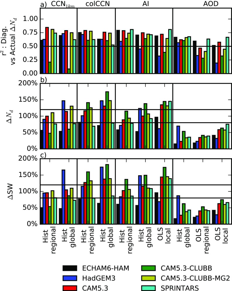
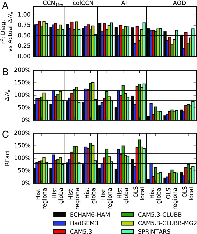
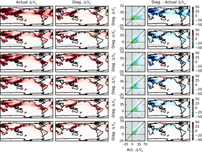
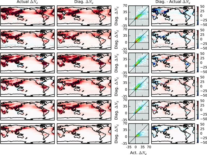
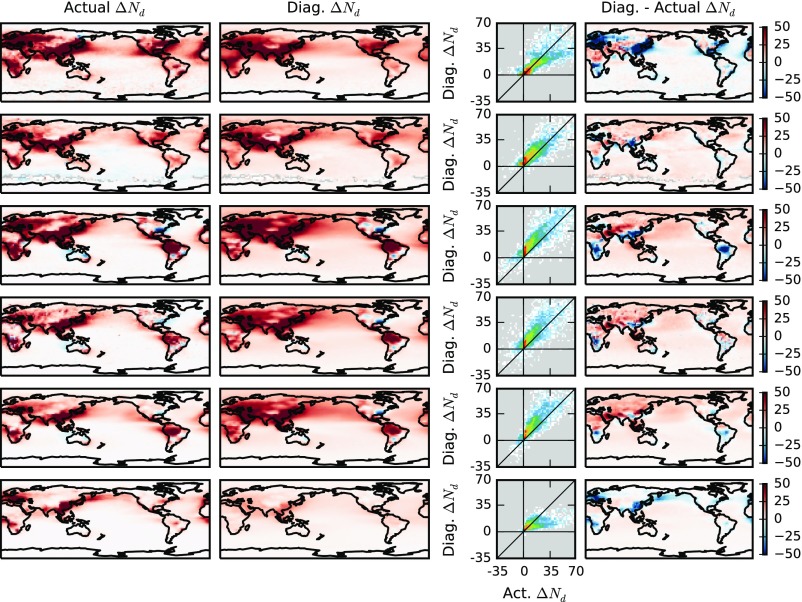
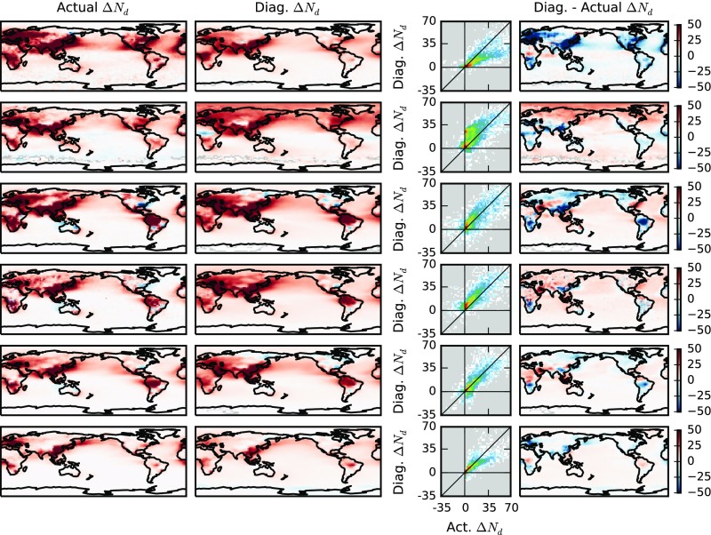
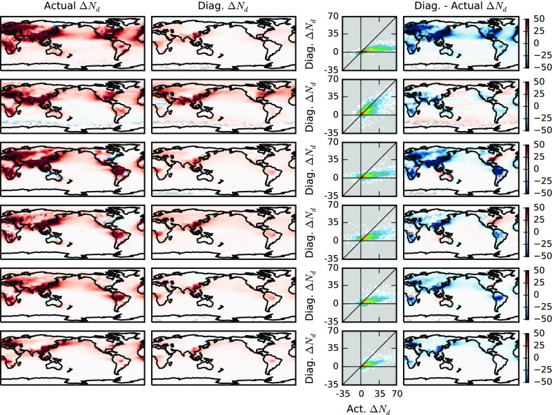
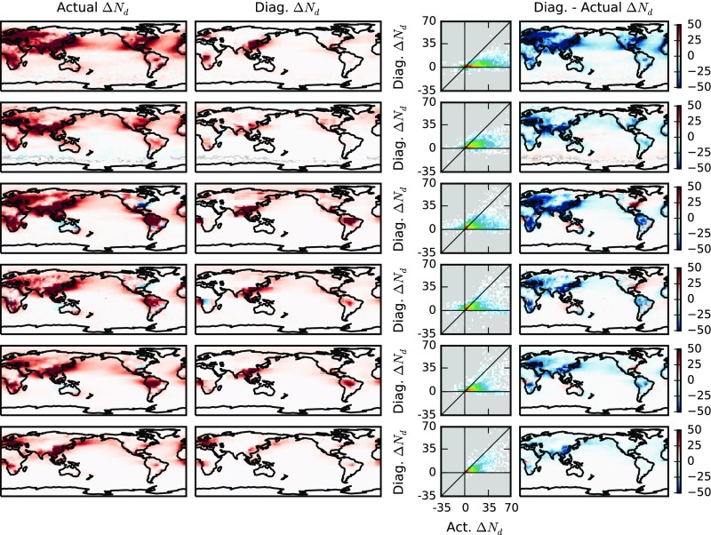
There is a good correspondence between the diagnosed and the actual $\mathrm{\Delta }{N}_d$ (Fig. 2, third column). The correlation coefficients between the diagnosed and actual $\mathrm{\Delta }{N}_d$ are between 0.84 and 0.92, explaining between 70% and 85% of the variance (Fig. 3A). These correlations decrease slightly if a single global joint histogram is used (Fig. 3A). The difference between the diagnosed and the actual $\mathrm{\Delta }{N}_d$ in the fourth column of Fig. 2 varies between the models, partially due to remaining difference between the daily mean CCN_1km and the cloud-base CCN. This seems to be important for the ECHAM6-HAM simulation over ocean (Fig. 2), where the 1-km level is more often above the cloud tops in stratocumulus regions (20) than in the other models. Repeating the analysis using the total column CCN at 0.3% supersaturation (“colCCN”) improves the $\mathrm{\Delta }{N}_d$ and RFaci diagnosis for ECHAM6-HAM (Fig. 3 B and C), possibly due to the extra information provided about cloud-base CCN. Regime-dependent updrafts may also play a role in controlling the remaining 20% of the variability in $\mathrm{\Delta }{N}_d$ (Fig. 3B). It is possible that there is further variability in $\mathrm{\Delta }{N}_d$ from PI–PD differences in the parameterized updrafts (which might be reduced by the nudging procedure), but this is a small component of the total variability and so is not further considered in this analysis. These results show that through the ability of the PD CCN_1km–N_d relationship to provide information on the “actual” CCN_1km–N_d relationship, the PD relationship can be used to provide an accurate estimate of the $\mathrm{\Delta }{N}_d$ due to anthropogenic aerosol perturbations, as long as that perturbation is known.

Fig. 3.

Comparison of different methods and proxies for calculating $\mathrm{\Delta }{N}_d$. “Hist” indicates the use of a joint histogram and “OLS” the use of an ordinary least-squares regression. (A) The determination coefficient between the diagnosed and the actual values of the $\mathrm{\Delta }{N}_d$ at a 2.5° by 2.5° resolution globally. (B) The relative size of the global mean $\mathrm{\Delta }{N}_d$. (C) The relative size of the implied global mean RFaci, with a percentage less than 100% indicating an underestimate in the estimated RFaci. The horizontal bars are at 80% and 120%. The plots summarized in this figure are shown in Figs. S2–S10.

Comparison of Aerosol Proxies.

Although $\mathrm{\Delta }{N}_d$ can be diagnosed through the PD CCN_1km–N_d relationship, observations of CCN_1km are sparse in both space and time, necessitating the use of other aerosol proxies for diagnosing $\mathrm{\Delta }{N}_d$. The aerosol index [AI, AOD multiplied by the Ångström exponent (4)] is routinely observed by satellites and provides more information about aerosol size than the AOD. Although not currently retrieved by satellites, colCCN provides extra information about the aerosol chemistry. For each of these proxies, the determination coefficient ($r^2$) between the diagnosed and the actual $\mathrm{\Delta }{N}_d$ is shown in Fig. 3A (see Figs. S2–S10 for other aerosol proxies). For comparison with earlier work, linear regressions between the N_d and aerosol proxies are also used to characterize the PD aerosol–N_d relationship (OLS). The relationships are determined at several different scales: 2.5° by 2.5° (“local”), 15° by 15° (“regional”), and a single global relationship (“global”). The local scale is only used with the OLS method, as there are not enough data within each grid box to generate a full joint histogram.

Fig. S2.

As Fig. 2, but using a single global CCN–N_d histogram (Hist CCN Global).

Fig. S10.

As Fig. 2, but using AI instead of the boundary layer CCN and a linear least-squares regression for each grid box instead of a joint histogram (OLS AOD local).

Fig. S3.

As Fig. 2, but using column-integrated CCN instead of the boundary layer CCN (Hist colCCN regional).

Fig. S4.

As Fig. 2, but using column integrated CCN and a single global joint histogram (Hist colCCN global).

Fig. S5.

As Fig. 2, but using AI instead of the boundary layer CCN (Hist AI regional).

Fig. S6.

As Fig. 2, but using AI and a single global joint histogram (Hist AI global).

Fig. S7.

As Fig. 2, but using AI instead of the boundary layer CCN and a linear least squares regression for each grid box instead of a joint histogram (OLS AI local).

Fig. S8.

As Fig. 2, but using AOD and a single global joint histogram (Hist AOD global).

Fig. S9.

As Fig. 2, but using AI instead of the boundary layer CCN and a linear least-squares regression instead of a joint histogram (OLS AOD regional).

Using separate regional PD joint histograms between CCN_1km and N_d (Fig. 3A, Hist regional) is best able to predict $\mathrm{\Delta }{N}_d$ for each of the models investigated here (excluding ECHAM6-HAM). A single global joint CCN_1km–N_d histogram (Hist global) results in a slight decrease in the ability to predict $\mathrm{\Delta }{N}_d$. There is again a slight weakening in predictive ability when moving to the colCCN as a proxy for diagnosing $\mathrm{\Delta }{N}_d$. The AI also provides a reasonable parameter for characterizing the aerosol, in many cases producing an accurate estimate of $\mathrm{\Delta }{N}_d$ (Fig. 3B). Using regional AI–N_djoint histograms for diagnosing $\mathrm{\Delta }{N}_d$ gives r² values between the diagnosed and the actual $\mathrm{\Delta }{N}_d$ (0.61 to 0.81) approaching those of the CCN_1km. Because the models do not provide the RFaci, the relative error in the RFaci is estimated by weighting $\mathrm{\Delta }{N}_d$ by the observed liquid cloud fraction and cloud albedo susceptibility (Fig. 3C, see Materials and Methods for details). In general, the regional joint histograms provide a more accurate diagnosis of RFaci, although using a single global histogram results in only a small increase in the error, even though the r² value decreases for all of the models (Fig. 3A). The AOD performs worst as a parameter for characterizing aerosol in the models when diagnosing $\mathrm{\Delta }{N}_d$ and RFaci. The local linear regressions have the lowest r² values of all of the methods and proxies investigated, although the RFaci estimate when using AOD is slightly improved compared with the regional linear regression, possibly due to the reduced aerosol type variability for a local regression (Fig. 3C).

From these results, it is clear that estimates of the aerosol forcing that rely on the relationship between AOD and N_d for characterizing the strength of aerosol–cloud interactions (such as many observational estimates) are likely to underestimate the anthropogenic perturbation of N_d by at least 30% (up to 90%). This would lead to an underestimate in the strength of the radiative forcing from aerosol indirect effects in these studies of at least 20% (up to 90%).

Satellite-Based Estimate.

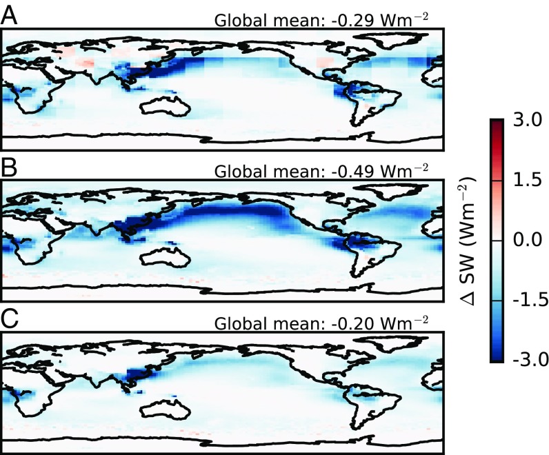
Although using the AOD as an aerosol proxy can lead to an underestimate when diagnosing the aerosol forcing, the AI is almost as good a proxy for the aerosol as the CCN_1km when attempting to diagnose $\mathrm{\Delta }{N}_d$ and the RFaci (Fig. 3C). Given this improved accuracy compared with using AOD as an aerosol proxy, AI and N_d data from the moderate-resolution imaging spectroradiometer (MODIS) are used to generate both regional joint histograms (Hist AI regional, 15° by 15° regions) and a single global joint histogram (Hist AI global), using 10 y of data (2004–2013). These are then combined with the annual mean MODIS liquid cloud fraction and the cloud susceptibility derived from MODIS and Clouds and the Earth’s Radiant Energy System (CERES) (Eq. 3) to provide an updated estimate of the RFaci (Fig. 4).

Fig. 4.

The mean of the individual model RFaci estimates (Fig. S11), using MODIS data to create (A) regional histograms, (B) a single global AI–N_d histogram, and (C) a single global AOD–N_d histogram, combined with model estimates of the anthropogenic AI/AOD contribution.

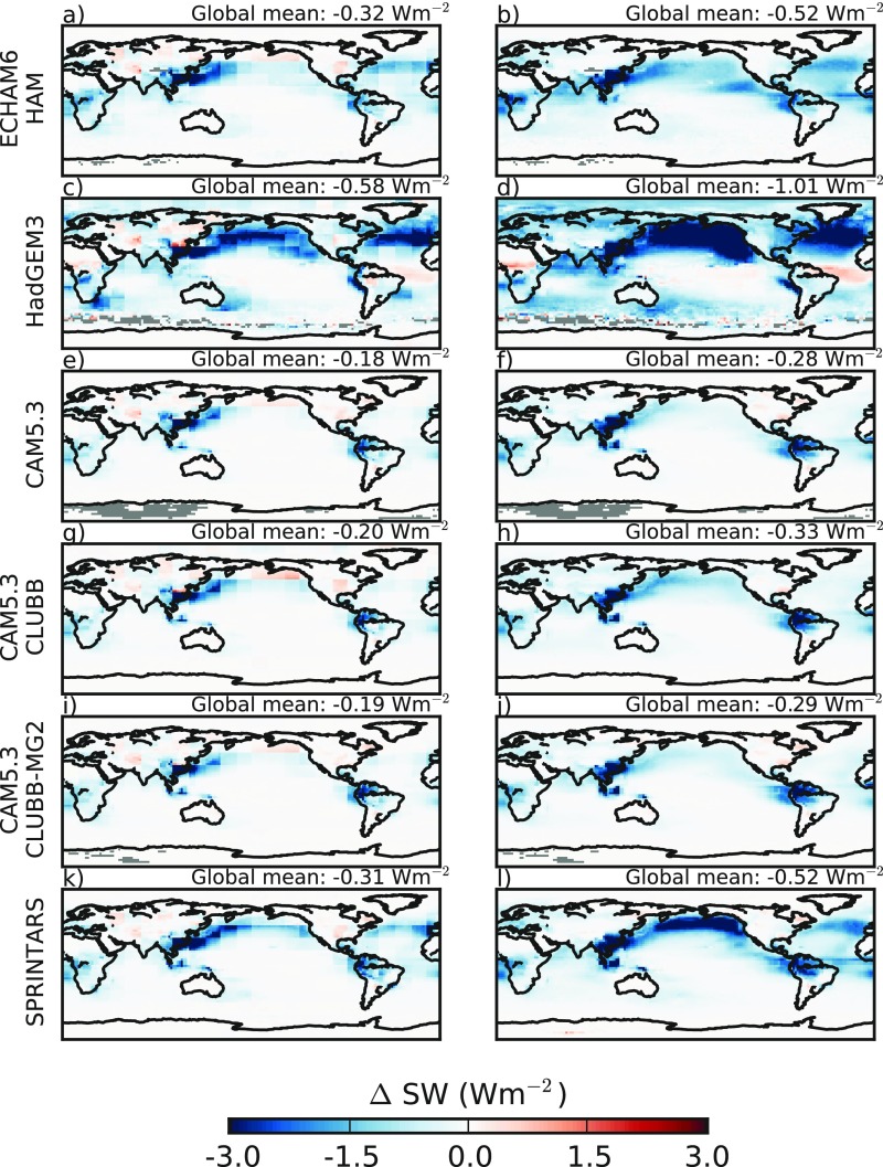
Using the PI-to-PD AI changes from each of the models gives a range of RFaci estimates for the regional method between −0.18 and −0.58 Wm⁻² and between −0.29 and −1.01 Wm⁻² if using a single global AI–N_d joint histogram (Fig. S11). The RFaci is generally higher over the ocean due to the higher liquid cloud fraction and cloud susceptibility, despite the smaller oceanic $\mathrm{\Delta }{N}_d$ (Fig. 2). Although this is not a large selection of models, the mean value of −0.29 Wm⁻² for the regional method and −0.49 Wm⁻² for the global histogram are instructive to compare with the −0.2 Wm⁻² mean value using a single global AOD-N_d histogram (Fig. 4C), −0.2 Wm⁻² using local OLS with AOD (7) and −0.4 Wm⁻² using local OLS and AI (21).

Fig. S11.

The SW radiative forcings diagnosed using the anthropogenic AI estimates from each of the included models with the Hist AI regional method (Left) and the Hist AI global method (Right). The latitude-weighted mean is shown at the top of each subplot.

There are some caveats to this estimate. First, the MODIS AI has little quantitative skill over land (22) and in some regions a positive RFaci is diagnosed from changes in the N_d (Fig. 4). This has a larger impact on the regional histogram method and may result in a reduction in the strength of the implied aerosol forcing. However, only a small fraction of the forcing comes from continental regions, similar to the findings from ref. 7, so this may not result in a large bias in the global mean RFaci. Also, the global histogram method is more likely to overestimate the RFaci (Fig. 3C), suggesting that the actual value is between the two estimates, perhaps around −0.4 Wm⁻² (this only includes changes to cloud albedo and not other rapid cloud adjustments). It is also possible that systematic biases in the MODIS AI or N_d retrieval could further affect this result, although the magnitude and sign of these effects is unclear. It should also be noted that this estimate is strongly dependent on the estimate of the anthropogenic aerosol fraction. Because all of the AeroCom models in this work use the same emissions database, the diversity in the forcing estimates from the models is unlikely to fully represent the full uncertainty in the radiative forcing from changes in cloud albedo.

Discussion

Previous work has shown that the PD CCN–N_d relationship sampled from spatiotemporal variability is not necessarily representative of the “actual” sensitivity of N_d to aerosol changes since the PI. This is partially due to the large errors in the sensitivity of the N_d to CCN in clean regions, where there is little CCN variation and consequently little N_d variation in the PD climate. However, these regions are usually regions with a small anthropogenic CCN contribution and so make only a small contribution to the global $\mathrm{\Delta }{N}_d$. Although the nudging process might reduce the variability in $\mathrm{\Delta }{N}_d$ from variations in the in-cloud updrafts, this work demonstrates that the CCN_1km–N_d relationship is representative enough in regions where there is a large $\mathrm{\Delta }{N}_d$ to make an accurate prediction of the global $\mathrm{\Delta }{N}_d$ and RFaci.

It is also interesting to note that the big increases in N_d occur in regions with large changes in CCN (over land, the Northern Hemisphere) in all of the models investigated here (Fig. 2). Although these models implement aerosol activation parameterizations that result in a saturation of the N_d at high CCN concentrations, this behavior is not evident in many of the joint histograms of Fig. 1 for the CCN_1km versus the N_d. Although there are other nonlinearities in the pathway between CCN changes and a change in top-of-atmosphere albedo (e.g., ref. 11), strong aerosol–cloud interaction effects also occur in regions of stronger aerosol perturbation for the CMIP5 models (albeit less concentrated in the Northern Hemisphere) (23), supporting the idea that the RFaci in remote regions such as the southern ocean does not dominate the total RFaci.

Finally, the results of this work demonstrate the importance of including aerosol size information when making estimates of the aerosol impact on cloud properties. Previous work has shown that the AI correlates better than the AOD with the cloud-base CCN (15). This work shows that it also offers significant benefits as an aerosol proxy when calculating $\mathrm{\Delta }{N}_d$ and the radiative forcing from aerosol–cloud interactions. The large increase in predictive ability of $\mathrm{\Delta }{N}_d$ when moving from AOD to AI for characterizing the aerosol shows the importance of a measure of aerosol size, especially given the strong changes in aerosol type between the PI and the PD simulations. Although there is also a clear benefit from including vertical information (CCN_1km is a better proxy than colCCN for most GCMs), this increase in the accuracy when diagnosing the radiative forcing is smaller than that when using AI compared with AOD. The change in predictive ability when moving from AI to column-integrated CCN is the smallest change, suggesting that information on aerosol composition is the least important of the three factors (vertical location, size distribution, and composition) that limit the ability of the AOD–N_d relationship to characterize the strength of aerosol–cloud interactions (24).

Conclusions

In this work, multiple aerosol–climate models have been used to investigate how a change in N_d can be predicted from PD aerosol–cloud relationships.

The use of joint histograms normalized by aerosol occurrence is demonstrated, accounting for nonlinearities in the aerosol–N_d relationship. It also removes the influence of the aerosol environment on the strength of the aerosol–N_d relationship, such that the PD and PI aerosol–N_d relationships are nearly identical with the correct choice of aerosol proxy (Fig. 1).

Although diagnosing the true sensitivity of N_d to CCN remains a difficult problem using only PD relationships (18), determining $\mathrm{\Delta }{N}_d$ is much easier because it weights the calculation toward regions with a larger change in CCN, where the relationship can be determined with greater accuracy (Fig. 2). If the change in CCN at 1-km altitude (CCN_1km) between the PI and the PD is known, then the PD relationship between CCN_1km and the N_d is enough to diagnose the PD–PI change in N_d ($\mathrm{\Delta }{N}_d$) to within 20% of the value determined by the climate simulations (Fig. 3). Using joint histograms to account for nonlinearities in the CCN–N_d relationship, a single global relationship between CCN_1km and N_d can be used, with only a small reduction in the accuracy of diagnosing $\mathrm{\Delta }{N}_d$ and the instantaneous radiative forcing due to changes in cloud albedo (RFaci).

Although vertical information is shown to be important in predicting $\mathrm{\Delta }{N}_d$, these results imply that information about the aerosol size distribution makes a dominant contribution to the accuracy of the predictions of $\mathrm{\Delta }{N}_d$, with the AI showing significant gains over the AOD, similar to previous work (15). The estimates of the anthropogenic change in AI provided by the models in this work combined with AI–N_d joint histograms from satellite data provide a revised RFaci estimate of around −0.4 Wm⁻², although there is a large diversity between the model estimates, ranging from −0.18 to −1.01 Wm⁻². The larger $\mathrm{\Delta }{N}_d$ suggested by this work also suggests a larger ERFaci than previous studies (11), but this is not investigated here. Because estimates of the PD–PI aerosol environment are often generated from models, estimates of the PD–PI AI change could be calculated alongside AOD changes. Using AI has the advantage over using CCN because it is currently retrieved by satellite instruments [although retrieving CCN may be possible in certain situations (25)]. This suggests that the AI is potentially a useful parameter to use when calculating observational constraints on the strength of RFaci in liquid clouds and where possible should be considered for future observation-based investigations.

Materials and Methods

Throughout this work, output from several global aerosol–climate simulations performed as part of the AeroCom model intercomparison project (18, 19) is used to provide simulations of the PD and PI atmospheres. Both PD and PI simulations are nudged to the same horizontal winds (2006–2010) and include PD greenhouse gases, sea surface temperatures, and natural forcings. All of the models include interactive aerosol modules that interact with the cloud via a modification of N_d, ice crystal number concentration, and radiative fluxes. This affects the radiation as well as the precipitation formation in liquid clouds via autoconversion, leading to more complex effects on the cloud properties. The model data are regridded to a 2.5° by 2.5° resolution and averaged to daily temporal resolution. Because this analysis focuses on liquid water clouds, only grid boxes with an ice water path of less than 5 g $\cdot$ m⁻² are used. Six of the nine available simulations were selected to provide a wide selection of models and microphysics schemes. The models themselves are self-consistent, such that an imperfect modeling of the aerosol or the cloud properties does not affect the conclusions.

$\mathrm{\Delta }{N}_d$ is diagnosed for each 2.5° by 2.5° grid box using the PD relationship between the aerosol parameter (A) and the N_d and the known change in the aerosol parameter between the PD and PI simulations. Eq. 1 shows how $\mathrm{\Delta }{N}_d$ is diagnosed within each grid box using a joint probability histogram between the aerosol and N_d created from PD relationships and the probability histograms of the PI and PD aerosol parameter in each grid box:

$$\mathrm{\Delta }{N}_d=\sum _{N_d}{N}_d\sum _{A}P{(N_d|A)}_{PD}\times (P{\left(A\right)}_{PD}-P{\left(A\right)}_{PI}).$$ [1]

If the OLS method is used, the calculation for $\mathrm{\Delta }{N}_d$ is conceptually similar, using the ACI metric $\left(AC{I}_A={\frac{d{N}_d}{dln(A)}}_{PD}\right)$ from ref. 5:

$$\mathrm{\Delta }{N}_d=AC{I}_A\times \left(\overline{\ln (A_{PD})}-\overline{\ln (A_{PI})}\right),$$ [2]

where the overbar denotes an average over a distribution. To investigate the impact that errors in diagnosing $\mathrm{\Delta }{N}_d$ have on the RFaci, the Twomey formula (26) is used to calculate the change in cloud albedo (${\alpha }_{cld}$). The cloud albedo is calculated from the CERES TOA SW all-sky albedo and the MODIS Aqua L3 (MYD08_D3) collection 6 cloud optical properties cloud fraction (27), using only grid boxes with zero ice cloud. This is combined with the MODIS annual mean liquid cloud fraction ($f_{liq}$) and the down-welling solar flux ($F^{\downarrow }$) to produce a simple estimate of the RFaci ($\mathrm{\Delta }{F}^{\uparrow }$) (28):

$$\mathrm{\Delta }{F}^{\uparrow }=-F^{\downarrow }{f}_{liq}\frac{{\alpha }_{cld}(1-{\alpha }_{cld})}{3N_d}\mathrm{\Delta }{N}_d.$$ [3]

The MODIS AI is used to provide an observational constraint on the RFaci by generating AI–N_d joint histograms from observations. For these histograms, the N_d is calculated using the adiabatic approximation, as specified in ref. 11. The AI is calculated from the AOD–Ångström exponent joint histogram in the MODIS MYD08_D3 product using only grid boxes where no ice cloud is detected (to reduce possible cirrus contamination). Because the relative error of the MODIS AOD and hence the Ångström exponent and AI is large at low AOD (<0.03), the N_d is assumed constant at AI values below 0.03.

References

- 1.Boucher O, et al. In: Clouds and Aerosols. Stocker T, et al., editors. Cambridge Univ Press; Cambridge, UK: 2013. pp. 571–658. [Google Scholar]
- 2.Twomey S. Pollution and the planetary albedo. Atmos Environ. 1974;8:1251–1256. [Google Scholar]
- 3.Albrecht B. Aerosols, cloud microphysics, and fractional cloudiness. Science. 1989;245:1227–1230. doi: 10.1126/science.245.4923.1227. [DOI] [PubMed] [Google Scholar]
- 4.Nakajima T, Higurashi A, Kawamoto K, Penner J. A possible correlation between satellite-derived cloud and aerosol microphysical parameters. Geophys Res Lett. 2001;28:1171–1174. [Google Scholar]
- 5.Feingold G, Eberhard WL, Veron DE, Previdi M. First measurements of the Twomey indirect effect using ground-based remote sensors. Geophys Res Lett. 2003;30:1287. [Google Scholar]
- 6.Koren I, Kaufman Y, Rosenfeld D, Remer L, Rudich Y. Aerosol invigoration and restructuring of Atlantic convective clouds. Geophys Res Lett. 2005;32:L14828. [Google Scholar]
- 7.Quaas J, Boucher O, Bellouin N, Kinne S. Satellite-based estimate of the direct and indirect aerosol climate forcing. J Geophys Res. 2008;113:D05204. [Google Scholar]
- 8.Quaas J, Stevens B, Stier P, Lohmann U. Interpreting the cloud cover - aerosol optical depth relationship found in satellite data using a general circulation model. Atmos Chem Phys. 2010;10:6129–6135. [Google Scholar]
- 9.Grandey BS, Gururaj A, Stier P, Wagner TM. Rainfall-aerosol relationships explained by wet scavenging and humidity. Geophys Res Lett. 2014;41:5678–5684. [Google Scholar]
- 10.Jones TA, Christopher SA, Quaas J. A six year satellite-based assessment of the regional variations in aerosol indirect effects. Atmos Chem Phys. 2009;9:4091–4114. [Google Scholar]
- 11.Gryspeerdt E, Quaas J, Bellouin N. Constraining the aerosol influence on cloud fraction. J Geophys Res. 2016;121:3566–3583. [Google Scholar]
- 12.Quaas J, et al. Aerosol indirect effects - general circulation model intercomparison and evaluation with satellite data. Atmos Chem Phys. 2009;9:8697–8717. [Google Scholar]
- 13.Bellouin N, et al. Impact of the modal aerosol scheme GLOMAP-mode on aerosol forcing in the Hadley Centre global environmental model. Atmos Chem Phys. 2013;13:3027–3044. [Google Scholar]
- 14.Shinozuka Y, et al. The relationship between cloud condensation nuclei (CCN) concentration and light extinction of dried particles: indications of underlying aerosol processes and implications for satellite-based CCN estimates. Atmos Chem Phys. 2015;15:7585–7604. [Google Scholar]
- 15.Stier P. Limitations of passive remote sensing to constrain global cloud condensation nuclei. Atmos Chem Phys. 2016;16:6595–6607. [Google Scholar]
- 16.Kaufman YJ, et al. Aerosol anthropogenic component estimated from satellite data. Geophys Res Lett. 2005;32:17804. [Google Scholar]
- 17.Penner JE, Xu L, Wang M. Satellite methods underestimate indirect climate forcing by aerosols. Proc Natl Acad Sci USA. 2011;108:13404–13408. doi: 10.1073/pnas.1018526108. [DOI] [PMC free article] [PubMed] [Google Scholar]
- 18.Ghan S, et al. Challenges in constraining anthropogenic aerosol effects on cloud radiative forcing using present-day spatiotemporal variability. Proc Natl Acad Sci USA. 2016;113:5804–5811. doi: 10.1073/pnas.1514036113. [DOI] [PMC free article] [PubMed] [Google Scholar]
- 19.Zhang S, et al. On the characteristics of aerosol indirect effect based on dynamic regimes in global climate models. Atmos Chem Phys. 2016;16:2765–2783. [Google Scholar]
- 20.Nam C, Bony S, Dufresne JL, Chepfer H. The ‘too few, too bright’ tropical low-cloud problem in CMIP5 models. Geophys Res Lett. 2012;39:L21801. [Google Scholar]
- 21.Lebsock M, Stephens G, Kummerow C. Multisensor satellite observations of aerosol effects on warm clouds. J Geophys Res. 2008;113:D15205. [Google Scholar]
- 22.Levy R, et al. Global evaluation of the collection 5 MODIS dark-target aerosol products over land. Atmos Chem Phys. 2010;10:10399–10420. [Google Scholar]
- 23.Zelinka MD, Andrews T, Forster PM, Taylor KE. Quantifying components of aerosol-cloud-radiation interactions in climate models. J Geophys Res. 2014;119:7599–7615. [Google Scholar]
- 24.Dusek U, et al. Size matters more than chemistry for cloud-nucleating ability of aerosol particles. Science. 2006;312:1375–1378. doi: 10.1126/science.1125261. [DOI] [PubMed] [Google Scholar]
- 25.Rosenfeld D, et al. Satellite retrieval of cloud condensation nuclei concentrations by using clouds as CCN chambers. Proc Natl Acad Sci USA. 2016;113:5828–5834. doi: 10.1073/pnas.1514044113. [DOI] [PMC free article] [PubMed] [Google Scholar]
- 26.Twomey S. Aerosols, clouds and radiation. Atmos Environ. 1991;25:2435–2442. [Google Scholar]
- 27.Platnick S, et al. The MODIS cloud products: Algorithms and examples from Terra. IEEE Trans Geosci Remote Sens. 2003;41:459–473. doi: 10.1109/TGRS.2016.2610522. [DOI] [PMC free article] [PubMed] [Google Scholar]
- 28.Charlson RJ, et al. Climate forcing by anthropogenic aerosols. Science. 1992;255:423–430. doi: 10.1126/science.255.5043.423. [DOI] [PubMed] [Google Scholar]