Robust Microbiota-Based Diagnostics for Inflammatory Bowel Disease

ABSTRACT

Strong evidence suggests that the gut microbiota is altered in inflammatory bowel disease (IBD), indicating its potential role in noninvasive diagnostics. However, no clinical applications are currently used for routine patient care. The main obstacle to implementing a gut microbiota test for IBD is the lack of standardization, which leads to high interlaboratory variation. We studied the between-hospital and between-platform batch effects and their effects on predictive accuracy for IBD. Fecal samples from 91 pediatric IBD patients and 58 healthy children were collected. IS-pro, a standardized technique designed for routine microbiota profiling in clinical settings, was used for microbiota composition characterization. Additionally, a large synthetic data set was used to simulate various perturbations and study their effects on the accuracy of different classifiers. Perturbations were validated in two replicate data sets, one processed in another laboratory and the other with a different analysis platform. The type of perturbation determined its effect on predictive accuracy. Real-life perturbations induced by between-platform variation were significantly greater than those caused by between-laboratory variation. Random forest was found to be robust to both simulated and observed perturbations, even when these perturbations had a dramatic effect on other classifiers. It achieved high accuracy both when cross-validated within the same data set and when using data sets analyzed in different laboratories. Robust clinical predictions based on the gut microbiota can be performed even when samples are processed in different hospitals. This study contributes to the effort to develop a universal IBD test that would enable simple diagnostics and disease activity monitoring.

INTRODUCTION

Inflammatory bowel disease (IBD), which encompasses ulcerative colitis (UC) and Crohn's disease (CD), is characterized by chronic inflammation of the gastrointestinal (GI) tract. IBD is a multifactorial disease attributed to a combination of genetic predisposition and environmental risk factors (1–3). The apparent increase in some of these risk factors is thought to have led to the emergence of IBD as a global disease with increasing incidence and prevalence (4). Pediatric patients account for 20 to 25% of the overall number of newly diagnosed cases, underlining the importance of IBD diagnosis by pediatricians (5). This diagnosis is complex, requiring a combination of clinical, biochemical, radiological, endoscopic, and histological tests (6), which often leads to a delayed diagnosis that may result in a reduced response to medical therapy and a higher incidence of surgical intervention (7). However, there is another emerging indicator of IBD that can be obtained quickly and easily, i.e., the intestinal microbiota.

Strong evidence links microbial colonization of the gut to the development of IBD, suggesting that intestinal inflammation results from interaction of the gut microbiota with the mucosal immune compartments (8–10). Substantial alterations in the composition and decreased complexity of the gut microbial ecosystem are common features in IBD patients (11). The utility of microbial signatures for prediction of clinical outcomes was recently demonstrated in pediatric IBD patients (12, 13) and specifically in CD patients (14). As a noninvasive, cost-effective technique, microbiota-based diagnostics hold great potential for the prevention of exacerbations and for early-stage disease detection. However, despite the recent developments in molecular methods that allow circumvention of the inability to cultivate most gut microbiota species, microbiota-based diagnostics are not applied in clinical practice yet.

One of the main obstacles to the dissemination of this application is the lack of reproducibility of microbiota signatures between hospitals and laboratories (15, 16). Advanced molecular techniques commonly used for microbiota analysis, such as next-generation sequencing, have been shown to be highly sensitive to every step in the analysis, from sample collection through storage conditions to molecular procedures such as DNA isolation, primer selection, PCR settings, and choice of sequencing platform (15–18). Since these techniques are currently still difficult to implement in clinical practice in a cost- and time-efficient way, for microbiota analysis to become part of routine diagnostics, a standardized, reproducible, and easily applied technique is needed.

An alternative to sequencing is the IS-pro technique, which allows the detection of bacterial DNA and its taxonomic classification down to the species level on the basis of 16S-23S ribosomal interspace (IS) fragment length (19). Carrying out the IS-pro procedure requires infrastructure and skills that are commonly found in every diagnostic lab. Moreover, the procedure is suited for routine diagnostic use and results are available within hours. In recent years, IS-pro has been extensively optimized and validated and has become an effective method for standardized gut microbiota profiling (20, 21). While IS-pro profiles have already been shown to be effective as clinical predictors (22), for universal application in routine diagnostics, clinical predictions need to be robust to variations introduced by differences in the laboratories, hospitals, technicians, and equipment employed.

In this study, we investigated the between-hospital reproducibility of IS-pro data and the effect of different perturbations on the outcome of clinical prediction models. We formulated the most probable perturbations, simulated them in the microbial profiles of a pediatric IBD cohort, and assessed their effects on predictive accuracy. Furthermore, we compared the effect across different classifiers to identify the classification algorithm that is least sensitive to potential perturbations and thus optimal for practical application. To assess the extent of perturbations in real life, we analyzed replicate data sets in two independent laboratories and estimated the predictive accuracy when a model was trained on one replicate and tested on the other, as would occur in clinical practice. On the basis of our simulations and validation in practice, we were able to identify which perturbations should be avoided and which classifiers are the most robust. The establishment of a reproducible tool for microbiota-based clinical predictions is a crucial step toward a universal diagnostic application.

RESULTS

Data set assessment.

This study was based on a cohort of 149 subjects, of which 91 were children diagnosed with IBD (consisting of 53 CD and 38 UC patients) and 58 were healthy children (designated A1). Two replicate data sets were generated on the basis of subsets of this data set, i.e., A2, consisting of 116 samples, of which 70 were IBD samples (from 28 CD and 42 UC patients) and the rest were controls, and M2, consisting of 30 samples, of which 20 were IBD samples (from 11 CD and 9 UC patients) and the rest were controls. A2, which was analyzed in the same laboratory as the original data set but with a different analysis platform, served as a platform replicate, whereas M2, which was analyzed in a different laboratory but with the same platform as A2, served as a hospital replicate (Fig. 1). Between-hospital replicate sample pairs clustered together (Fig. 2A) and were highly correlated (n = 28, median R² = 0.89 [interquartile range = 0.3]). The variation introduced by the analysis platform was larger than that introduced by the hospital, as shown in Fig. 2B.

FIG 1.

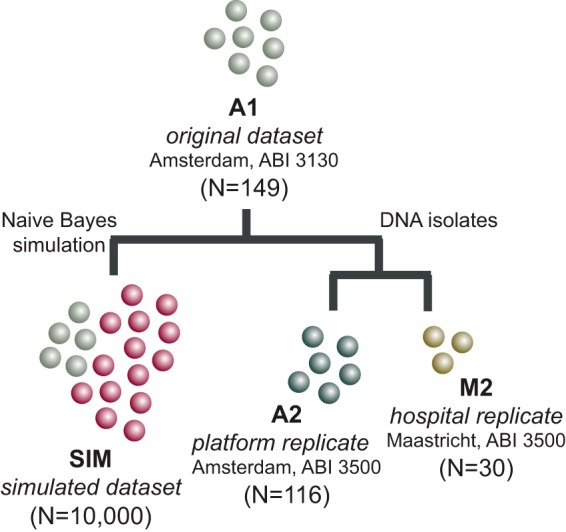
Study design. Four data sets were analyzed in this study. All data sets were generated on the basis of one original data set (A1) by either simulating new synthetic observations (SIM) or reanalyzing the DNA isolates with IS-pro in two independent laboratories (A2 and M2). For each nonsynthetic data set, the lab in which it was processed and the machine model with which it was analyzed are indicated.

FIG 2.

Replicate sample comparison. (A) Heat map of between-hospital replicates. Pairwise clustering is observed for all samples except one. Columns correspond to samples, and rows correspond to peaks (i.e., bacterial species). Clustering is based on the cosine correlation matrix of peak intensities by the unweighted pair group method using average linkages. nt, nucleotides. (B) Principal-coordinate analysis of samples of the original data set (A1) and its two replicates (A2 and M2). Samples are primarily grouped by analysis platform. Samples represented by green and pink dots were analyzed with the same machine model (ABI 3500 genetic analyzer), while samples represented by blue dots were analyzed with a different machine model (ABI PRISM 3130 genetic analyzer). The hospital is not a large source of variation. Samples represented by blue dots were analyzed in the same lab in Amsterdam, The Netherlands, while samples represented by pink dots were analyzed in a different lab in Maastricht, The Netherlands. The principal-coordinate analysis was based on between-sample cosine distances.

To improve the prediction models' quality and to gain better predictive performance, the original data set was extended with synthetic samples. This allowed us to avoid overfitting, which is one of the main concerns when fitting a high-dimensional model with only a small number of samples. We generated a complementary synthetic data set (designated SIM; for details, see Materials and Methods) consisting of 10,000 samples in total and balanced between the two classes, IBD and healthy. The original and synthetic data sets are displayed in Fig. 3A, demonstrating segregation between the two classes, while synthetic samples are grouped together with the original samples of the same class.

FIG 3.

IBD versus healthy gut microbiota samples. (A) PLS-DA components of the original samples (A1, filled circles) and the synthetic samples (empty circles). (B) Predictive accuracy displayed as receiver operating characteristic curves based on a 10-fold cross validation of the original data set (A1). The main curve illustrates the accuracy of IBD classification against healthy controls, whereas the two smaller curves illustrate the accuracy of each IBD subtype (UC or CD) against healthy controls. (C) A learning curve that was used to determine the optimal training set size. Each classifier was trained on synthetic data and tested on the original data set. Training sets of each size were repeatedly subsampled 10 times.

To validate the synthetic data set, we compared the distribution of each peak in the original data set to that in the synthetic data set. All resulting P values were 1 following a false discovery rate correction, which means that the resulting synthetic peaks' distributions were not statistically significantly different from those of the original data. We also calculated the concordance per class between the average original profile and the average synthetic profile using Kendall's coefficient of concordance. For both classes, high concordance values were obtained (0.9977 and 0.9951 for the healthy and IBD classes, respectively), which means that the synthetic profiles and the original profiles generally agree. On the basis of this assessment, the synthetic data set was regarded as valid for further experiments.

The predictive accuracy of the original data set was assessed by using seven different classifiers that obtained similar performance, with the area under the curve (AUC) ranging from 0.85 for L2-regularized logistic regression to 0.92 for nearest shrunken centroids (NSC) (Fig. 3B). Specifically, both IBD subtypes could be discriminated from healthy controls with high accuracy. UC classification achieved a maximal AUC of 0.96 (for NSC, random forest [RF], and L2-regularized logistic regression), and CD classification obtained a maximal AUC of 0.87 (for NSC and RF). UC and CD were taken together as a single IBD group since both presented similar variations (see below for details).

We used a learning curve of increasing training set sizes to assess the predictability of the synthetic data and to determine the optimal training set size that should be sampled. The accuracy of all classifiers increased as more samples were considered for training (Fig. 3C). On the basis of the moderating accuracy improvement observed toward the larger training sets, we determined that 400 training samples would be a valid size for subsequent simulations. For this sample size, the accuracy was also comparable to the accuracy achieved by cross-validation of the original data set.

Probing of variation boundaries.

This section of the study consists of synthetic data experiments aiming to explore the effects of different sources of variation on predictive accuracy. We estimated the effects of five simulated perturbations on the accuracy of seven classifiers and identified which classifiers were more robust and therefore may outperform others when applied in diagnostics.

(i) Single perturbations.

Each sample is represented as a microbial profile (Fig. 4). We formulated the perturbations that are most likely to occur between profiles processed in different runs (Table 1). Each of these was simulated with increasing extent as a variation of the SIM data set (see Materials and Methods). The following procedure was repeated 100 times. A balanced training set (400 samples) was subsampled from the SIM data set, and the rest of the samples were perturbed and used as a test set. With this setting, we assumed that a clinical prediction model would be trained on a reference data set but would be used to predict data generated in various diagnostic centers (therefore incorporating different sources of variation).

FIG 4.

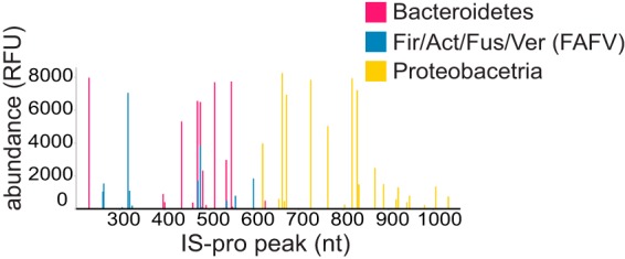
An IS-pro microbial profile example. Each sample in this study is represented as a microbial profile composed of peaks that correspond to different IS fragments. The IS fragment length (nucleotides [nt]) is depicted on the x axis, and bacterial species abundance is displayed on the y axis. Colors correspond to bacterial phylum group as amplified by IS-pro. Fir, Firmicutes; Act, Actinobacteria; Fus, Fusobacteria; Ver, Verrucomicrobia.

TABLE 1.

Detailed descriptions of the perturbations simulated in the SIM data set

Perturbation	Description
P1, intensity cutoff	Simulates effect of truncation of high peaks (e.g., by a technical cutoff)a
P2, peak shifts	Simulates random shifts in peak positions of ±1-nucleotide lengthsb
P3, intensity noise	Simulates addition of noise to all peak intensities
P4, peak deletion	Simulates the greater likelihood that low-intensity peaks will fall under the lower limit of detectionc
P5, dominant peak deletion	Simulates deletion of high-intensity peaksd

^aWith the rest of the peaks left intact.

^bThis may happen when continuous peak position values are binned into discrete variables during preprocessing.

^cEach peak was assigned a probability of being deleted, which was found in reverse ratio to its intensity.

^dWhile this perturbation is not likely to occur in reality, it gives an insight into the importance of high-intensity peaks for classification.

Figure 5 displays how predictions were affected by each individual perturbation. An intensity cutoff (perturbation 1 [P1]) did not have any effect on the predictive accuracy across all classifiers (Fig. 5A). Peak shifts (P2) and addition of intensity noise (P3) led to a gradual decrease in accuracy, with more peaks being perturbed (Fig. 5B and C). Still, the most pronounced effect was caused by peak deletion. When deleted peaks were mainly low-intensity peaks (P4), we observed a substantial decrease in predictive accuracy in all of the classifiers except RF (Fig. 5D). We further noted that deletion of four to seven peaks led to substantial variation between simulations, suggesting that it is important which particular peaks are deleted. With more peaks being deleted, the accuracy converged and the variation between different simulations was reduced.

FIG 5.

Effects of perturbations on the predictive accuracy of the SIM data set. Each panel represents the effect of a different perturbation, simulated with increased extent (depicted on the x axis) in the SIM data set. Training sets of 400 samples were repeatedly subsampled 100 times from the SIM data set, while the rest of the samples served as a test set. Classifiers were trained on unperturbed data and tested on perturbed data. Colors correspond to different classifiers. Gray bars reflect the actual observed amounts of between-hospital perturbations (between replicates A2 and M2, dark gray) and between-platform perturbations (between replicates A2 and A1, light gray). The perturbations tested were as follows: P1, intensity cutoff (A); P2, peak shifts (B); P3, intensity noise (C); P4, peak deletion (D); P5, dominant peak deletion (E). They are further elaborated in Table 1.

RF stood out with a response to the simulated perturbations distinct from that of the rest of the classifiers; it remained stable in response to the deletion of low-intensity peaks, while deletion of even a limited number of peaks led to a considerable decrease in accuracy for other classifiers (Fig. 5D). Even though it was affected when dominant peaks were deleted (P5), its accuracy decline was slower than that of the rest of the classifiers (Fig. 5E). On the other hand, the drop in its accuracy in response to intensity noise simulation was more pronounced than that of the rest of the classifiers (Fig. 5C).

(ii) Mixed perturbations.

We further explored the effect mixed perturbations have on predictive accuracy by using 100 variations of the SIM data set, each combining a random extent of every perturbation (excluding P5, as this is not a perturbation likely to occur in real data). Ten balanced training sets of 400 samples each were subsampled from every data set, while the rest of the samples were used as a test set. For each data set, we calculated the average cosine distance between the perturbed version of each sample and its unperturbed origin. Increased prediction error was observed as perturbed samples became less similar to their corresponding original samples, reflected by higher mean cosine dissimilarity (see Fig. S1 in the supplemental material). We identified several outlier data sets characterized by relatively high error rates for samples that were, on average, still quite similar to their origins (reflected by low mean cosine dissimilarity). Further investigation revealed that these outliers corresponded to data sets in which peak deletion (P4) affected more peaks, which led to a larger effect on prediction error. This is demonstrated in Fig. S1, where the marker size corresponds to the average number of deleted peaks and the outlier data sets are circled. The rest of the perturbations did not exhibit a similar relationship. RF, which proved robust to peak deletion, did not have any outlier data sets.

Between-hospital and between-platform variations.

Following our simulations, we investigated the batch effects on predictive accuracy by using replicate data sets reprocessed and analyzed in two independent hospitals with two different analysis platforms.

(i) Perturbation assessment.

Variation was estimated on the basis of the perturbations defined in Table 1 (P2, P3, and P4) by using pairwise comparisons of replicates and compared to the calculated simulated values (gray bars in Fig. 5B, C, and D). The between-platform batch effect (light gray bars in Fig. 5) appeared to be in the range where predictive accuracy is diminished by all three perturbations. The total number of peaks detected in a reference profile but missing from its corresponding replicate is shown in Fig. 6A, separated according to the type of perturbation. On average, more than half of the peaks in each pairwise comparison were missing (65%), out of which 35% were shifted peaks and 30% were deleted peaks.

FIG 6.

Analysis platform effect versus hospital effect on peak shifts and deletions. (A) The proportion of missing, shifted, or deleted peaks based on pairwise replicate comparisons. A peak is missing if it is detected in the reference profile but missing from its replicate. A missing peak can be either shifted or deleted. It is shifted if it is detected in the +1 or −1 position in the replicate profile. Otherwise, it is defined as “deleted.” *, P < 0.01; **, P < 0.001. (B) The proportion of deleted peaks per decile of peak intensity based on pairwise replicate comparisons.

The effect of between-hospital variation, however, depended on the type of perturbation. The number of shifted peaks (P2) and the difference in measured intensity (P3) were in the range where they had only a minor effect on predictive accuracy on the basis of our simulation, but the number of deleted peaks (P4) was in the range where predictive accuracy decreased for all classifiers, except RF (dark gray bars in Fig. 5). However, the proportion of missing peaks per pairwise comparison was significantly smaller than that observed for between-platform replicates (Fig. 6A, P < 0.001, Mann-Whitney U test). Missing peaks were sorted to either deleted or shifted (in case the peak was found in one of the adjacent positions in the replicate profile). The proportions of both deleted and shifted peaks were significantly smaller for between-hospital replicates than for between-platform replicates (Fig. 6A, P = 0.01 and P < 0.001, respectively; Mann-Whitney U test). The difference in measured intensity was also significantly smaller for between-hospital replicates than for between-platform replicates (P < 0.001, Mann-Whitney U test). Finally, we also assessed these perturbations separately for UC and CD to validate that no disease-specific batch effects were observed (see Fig. S2).

Since our simulations showed that the intensity value of a deleted peak (i.e., low or high) determines the effect on accuracy, we examined the intensity distribution of deleted peaks (Fig. 6B). This revealed that, as expected, the majority of deleted peaks had low intensity. Only two deleted peaks had intensity values that belonged to the top peak intensity decile in the entire between-hospital comparison.

(ii) Predictability assessment.

Subsequently, we assessed the accuracy of cross-platform and cross-hospital models by cross-validation. Each classifier was trained by using samples from one data set and tested on samples from a replicate data set. As a reference, we cross-validated the classifiers within the same data set (by using the same folds). All models were trained by using the A2 data set (n = 116), and the test set was limited to the 28 samples that were shared by all three data sets.

Figure 7A shows that while the cross-platform accuracy (blue) was relatively low, the cross-hospital accuracy (pink) was comparable to the within-data-set models' accuracy (green). A paired-prediction comparison of the three settings indicated that cross-platform predictions were significantly different from the within-data-set predictions for three out of seven classifiers (RF, NSC, L2-regularized logistic regression [q value of <0.03, McNemar's test]). However, cross-hospital predictions showed no significant differences from the within-data-set predictions for all classifiers. The number of predictions that did not agree, independently of their disease status, between within-data-set models and cross-hospital models is shown per classifier in Fig. 7B. RF had one misclassification in the within-data-set setting, while it could classify all samples correctly in the cross-hospital setting (1/28 mismatches). Partial least-squares discriminant analysis (PLS-DA), on the other hand, had a total of 7 mismatches (7/28) between the two settings.

FIG 7.

Cross-platform and cross-hospital prediction models. (A) Predictive accuracy based on cross-hospital (pink), cross-platform (blue), and within-data-set cross-validation (CV) (green) settings. All models were trained by using the A2 data set (n = 116) and tested on different data sets in a 10-fold CV (n = 28). (B) Comparison of correct (blue) and incorrect (pink) predictions per sample based on A2 within-data-set CV (top row) and cross-hospital CV (bottom row) settings. The total number of mismatches, i.e., where predictions disagree, is indicated at the top per classifier.

DISCUSSION

In this study we investigated batch effects of microbial profiles and how different sources of variation affect the accuracy of clinical prediction models. We studied between-hospital and between-platform variations by using replicate data sets and showed that while between-hospital variation occurred, it was less evident than between-platform variation. In addition, cross-hospital predictions, on the basis of models that were trained and tested by using data sets from different hospitals, showed performance similar to that of models cross-validated within the same data set. Finally, among all of the classifiers tested, RF proved to be the most robust classifier to both simulated and observed perturbations.

Gut microbiota profiles allowed prediction of the presence of IBD in pediatric patients. These predictions remained valid when a subset of samples was reprocessed and reanalyzed in a different hospital. While Papa et al. (12) achieved similar accuracy for pediatric IBD predictions, their results indicated that an important factor in diagnostic accuracy was the sequencing depth, which allows low-abundance but highly informative groups to be sampled. This might lead to increased costs, as fewer samples can be analyzed in every run. A diagnostic test based on the IS-pro technique is independent of the batch size and would therefore be more cost effective. The same authors also showed that blind validation with an independent patient sample confirmed the classification accuracy, which is crucial for a reliable model, but in contrast to our study, all of their samples were processed at the same lab.

Other multicenter studies or reanalyses that pooled several cohorts together to construct a prediction model for IBD did not attempt to test it in a cross-hospital setting (23, 24). While Gevers et al. (13) did construct a cross-hospital prediction model for CD based on a large multicenter cohort, all of the samples included were still stored, processed, and analyzed in the same center. The ability to reproduce the within-data-set accuracy with a between-hospital cross-validation is important, since batch effects are quite common in microbiota studies (15, 16). These effects have been shown to significantly impact predictive accuracy in microbiota-based predictive models of obesity (25) and CD (14).

It is recognized that significant intercenter differences in microbiota composition can be attributed to different PCR primers for 16S rRNA amplification or various sequencing platforms (16). This was recently demonstrated by Pascal et al. (14), who identified a unique microbial signature consisting of eight microbial markers for CD that was successfully validated in various different cohorts. However, when applied to a data set processed by a different methodological approach, their method achieved poor accuracy. In particular, two markers highly important for the discovered signature were either completely missing or found at very low abundance in this data set.

Such outcome variations are avoided with IS-pro, which uses standardized phylum-specific primers. Even though IS-pro is a highly standardized technique that uses common laboratory instruments, batch effects can still impact its results. For example, a large variation between replicates from different analysis platforms was observed. It is therefore important to systematically identify which factors may lead to batch effects large enough to impact predictive accuracy.

On the basis of our simulated perturbations, we determined that peak deletions had the greatest impact on predictive accuracy. The high variation in accuracy observed when four to seven peaks were deleted suggests that, in this range, the exact selection of deleted peaks is important to the classifier. Apparently, with a larger amount being deleted, the classifier loses enough information for its performance to deteriorate regardless of which peaks are missing. The rest of the simulated perturbations had a limited effect on accuracy, probably because they are more inherent to the data and so occur more often in the unperturbed form of the synthetic data set. Consequently, small variations in intensity and peak shifts are already considered by the classifier in the training phase.

RF appeared to be a robust classifier to handle peak deletions. RF is commonly used for microbiota classifications because of its accuracy and speed (12) and was shown to obtain the best performance of the classifiers studied across several benchmark data sets of human microbial communities (26). This can be explained by its mechanism. At each iteration of the construction of an RF, the estimator is based on a subset of input features, while part of the sample is left out by the bootstrap mechanism. The random subsampling could possibly reduce the effect of outliers. In our study, the robustness of RF was translated in practice to the highest achieved accuracy when tested in the cross-hospital setting and the smallest number of discrepancies between the cross-hospital predictions and the within-data-set cross validation.

The cross-sectional design of our study, which included fecal samples collected at the time of diagnosis and before any treatment had started, allows a good estimation of diagnostic accuracy while excluding confounding factors such as different treatment regimens. Furthermore, simulation of a large, balanced synthetic data set enabled a realistic estimate of the models' generalization error while circumventing sample size limitations, which are common to microbiota studies because of high dimensionality and high interindividual variation (25, 27). Additionally, on the basis of a comparison across seven classifiers, we were able to draw generalized conclusions that were not algorithm dependent and at the same time to identify algorithm-unique behavior, as was demonstrated in the case of RF.

Our study also had several limitations. First, we used healthy children as controls, whereas clinicians need to discriminate IBD patients from those with other GI complaints or diseases. As for the cases, we decided, on the basis of our classification and perturbations results, to combine UC and CD patients into one IBD group, even though they were recently described as two distinct subtypes of IBD at the microbiota level (14). In addition, all of the IBD patients in our cohort were in the active state of the disease, so our model cannot be extrapolated to a remission state of IBD. On the other hand, since an initial IBD diagnosis is performed when patients suffer from disease symptoms, our model is suitable for the most common situation. Our replicate data sets were limited to only two different platforms and two hospitals, and the between-hospital replicate data set was an unbalanced subset of the original cohort and rather small. Finally, since DNA extraction has been shown to be an important factor in microbiota composition variation (28, 29), our replicate data sets did not include reisolation of the DNA, rather than reprocessing of the same DNA isolates. The DNA isolates were therefore stored until the two replicates were analyzed, which may also introduce some degree of variation.

Our findings suggest that microbiota profiling by IS-pro is suitable for use as a diagnostic tool in clinical practice. Since the gut microbiota is a powerful IBD biomarker and IS-pro profiles proved to be accurate and robust predictors of the disease, our study shows that this technique may be used for the development of a universal diagnostic test for IBD based on a community characterization of the gut microbiota. This test should be analysis platform specific, and a robust algorithm like RF should be incorporated. Our analysis indicates that while the batch effect introduced by different hospitals is mostly expressed by means of peak deletions, RF was able to handle this kind of perturbation and maintained high accuracy. The next step in developing a universal IBD diagnostic test should be a large multicenter clinical study using independent IS-pro analyses at local laboratories to validate and further generalize our findings.

MATERIALS AND METHODS

Subjects and samples.

Children <18 years old and presenting with newly diagnosed, untreated UC or CD according to the current diagnostic Porto criteria for pediatric IBD were included in this study, which was performed between April 2010 and November 2014 in the tertiary hospitals of the VU University Medical Center (VUmc) and the Academic Medical Center (AMC) in Amsterdam, The Netherlands. Exclusion criteria were use of antibiotics, steroids, or immunosuppressive therapy within the last 3 months prior to inclusion; a previous diagnosis of IBD; a history of surgery of the GI tract (except appendectomy); and proven infectious colitis during the 3 months prior to inclusion. As a control group, a cohort of healthy Dutch children <18 years old previously described by de Meij and colleagues (20) was included. Fresh fecal samples were collected in sterile plastic containers and immediately stored in a freezer at −20°C. Patients undergoing diagnostic colonoscopy were instructed to collect a fecal sample prior to bowel preparation. This study was approved by the Medical Ethics Committee of VUmc and was performed in accordance with the ethical standards laid down in the 1964 Declaration of Helsinki and its later amendments.

Data sets and study design.

The original data set of this study was a cohort of 149 individuals of which 58 were healthy children and 91 were pediatric patients with IBD. This sample set was processed and analyzed in Amsterdam, The Netherlands, with an ABI PRISM 3130 genetic analyzer and was designated A1. This data set was used to generate three additional data sets, as illustrated in Fig. 1, i.e., a large synthetic data set (n = 10,000; see data simulation using a Gaussian mixture model), referred to here as SIM, and two replicate data sets using subsets of the original samples. The microbial profiles of both replicates result from reprocessing of the original DNA isolates, followed by a repeated PCR procedure and fragment analysis with an ABI 3500 genetic analyzer, in the original lab and in an independent lab at the department of medical microbiology of the Maastricht University Medical Center (MUmc), Maastricht, The Netherlands. These replicates were designated A2 and M2, respectively.

Microbiota profiling by IS-pro.

DNA was extracted from fecal samples with the easyMag extraction kit in accordance with the manufacturer's instructions (bioMérieux, Marcy l'Etoile, France). All DNA isolates were stored at 4°C. Samples were then analyzed with the IS-pro assay (IS-Diagnostics, Amsterdam, The Netherlands) in accordance with the protocol provided by the manufacturer, as described previously (18, 20). In short, IS-pro differentiates bacterial species by the length of the 16S-23S rRNA gene IS region with taxonomic classification by phylum-specific fluorescently labeled PCR primers. There are three phylum-specific primer sets for the phyla, (i) Bacteroidetes; (ii) Firmicutes, Actinobacteria, Fusobacteria, and Verrucomicrobia (FAFV); and (iii) Proteobacteria. DNA fragment analysis was originally performed on an ABI PRISM 3130 genetic analyzer (Applied Biosystems). For the replicate data set, 10 μl of each DNA isolate was sent in a cool pack to MUmc. All DNA isolates were then reanalyzed on an ABI 3500 genetic analyzer (Applied Biosystems) both at MUmc in Maastricht and at VUmc in Amsterdam (data sets M2 and A2, respectively).

Data preprocessing.

Preprocessing was carried out with the IS-Pro proprietary software suite (IS-Diagnostics Ltd.) and resulted in microbial profiles that are presented as peak profiles (Fig. 4). Each peak is characterized by a color that corresponds to the primer complementary to the amplified fragment and therefore corresponds to the phylum (or phylum group) from which it derives. The length of the IS fragment, measured in nucleotides, discriminates bacteria at the species level, and the peak intensity represents the amount of the PCR product, measured in relative fluorescence units (RFU). We considered each peak an operational taxonomic unit (OTU) and its intensity its abundance. Intensity values were log₂ transformed. Subsequently, OTUs and their corresponding abundances were used as features for supervised classification.

Data simulation with a Gaussian mixture model.

We used a generative naive Bayes model to simulate synthetic samples, since a larger data set prevents overfitting and allows a better estimation of the perturbations' effects by repeated subsampling of multiple different training sets. For each class (healthy or IBD), a Gaussian mixture model was fitted per feature by using the expectation-maximization algorithm with the sklearn.mixture package of the scikit-learn 0.16.0 Python library (30). Models were fitted with a diagonal covariance matrix and compared over 1 to 10 components. The model selected had the lowest Bayesian information criterion value. Feature values were then sampled by the model and combined to generate a new observation. All values of <6 log₂ RFU were set to 0. This simulation was used to complete the original data set to a total of 10,000 samples, balanced between healthy and IBD samples. The simulated data set was validated by (i) comparing the feature distributions of the original data set and the simulated data by using the Kolmogorov-Smirnov test, (ii) calculating the concordance correlation coefficient per class between the average profile of the original data set and that of the simulated data, and (iii) using a learning curve. We used supervised classification with training sets of increasing sizes (20 to 400 samples, repeatedly subsampled 10 times for each size) from the simulated data and the original data as the test set.

Perturbation simulations.

A peak x in a profile is defined as x = {x_p, x_i|x_p ϵ ℕ, x_i ϵ ℝ}, where x_p is the peak's position, which corresponds to the length in nucleotides of the IS fragment, and x_i is the peak's intensity, which corresponds to the amplified quantity of that fragment. We formulated the perturbations most likely to occur when IS-pro is run in different labs as follows. The first factor is intensity cutoff. For each peak {x|x_i > k}, where x_i is the peak's intensity measured in log₂ RFU and k ϵ {12, 12.5, 13, 14, 15}, we assigned x_i ← k. The second factor is peak shifts. A subset of n peaks, S_n, where n = kN, k ϵ {0.05, 0.1 … 0.4}, and N = |{x|x_i > 0}| is the total number of nonzero peaks in a profile, was randomly selected. For each peak {x|x ϵ S_n}, a shifted position was assigned by ${\text{x}}_{\text{p}}^{\text{new}}$←x_p ± 1. This simulates the fact that during the preprocessing of the profiles, continuous position values are binned into discrete peak positions, which may consequently result in variations of ±1 nucleotide in the peak position of the same OTU. The third factor is intensity noise. For each peak x, a new intensity value was assigned by ${\text{x}}_i^{\text{new}}$←max(x_i + ε_i, 0), where ε_i randomly sampled from UNIF$(-k\frac{\text{range}(\text{x})}{50},\hspace{0.17em}k\frac{\text{range}(\text{x})}{50})$, in which k ϵ {1, 5, 10, 15, 20, 22, 25} and range(x) = max_j(x_j) − min_j(x_j), is the difference between the maximum and the minimum intensity values of the peak in the SIM data set, as implemented in the R function jitter. The fourth factor is peak deletion. The probability that peak x will be deleted was defined as p(x_i ← 0) = $\frac{\min (x_i,k)}{x_i}$, where x_i is the peak's intensity measured in RFU and k ϵ {25, 50, 75, 100, 200, 30, 400}. This simulates the fact that low-intensity peaks have a higher probability of randomly falling below the lower limit of detection because of, e.g., variation in PCR efficiency. The fifth factor is dominant peak deletion. This perturbation was designed to investigate the effect deletion of high-intensity peaks would have on predictive accuracy, even though they are not prone to falling below the PCR assay's lower limit of detection. To simulate this, all peaks that belonged to the kth intensity percentile, k ϵ {0.995, 0.99, 0.985, 0.98}, were set to 0.

In all of the perturbations described, k was used as a parameter to control the extent of each perturbation in order to explore its varying effect on predictive accuracy in a series of discrete increasing steps.

Supervised classification.

We used supervised classification models to predict the health status of individuals on the basis of their gut microbiota profiles. For high-dimensional data, it is essential to control the variance of the model parameter estimates. This was achieved both by increasing the training set size with synthetic data and by applying regularization that constrains the size of the coefficients. The classifiers used were RF, NSC (31), elastic net (ENET) (32), L1- and L2-regularized logistic regression, PLS-DA, and L1-regularized L2 loss support vector machine (SVM).

RF, NSC, ENET, SVM, and PLS-DA have all been successfully applied in human microbiota classification tasks (22, 26), as well as in genomics, a field with similar dimensionality challenges (31–35). We used the following publicly available packages in the statistical software R: randomForest with default settings for the RF classifier; LiblineaR with type “L1-regularized L2-loss support vector classification” and the cost constant tuned by the heuristics provided by the heuristicC function for SVM; glmnet with α values of 0, 1, and 0.5 for L2- and L1-regularized logistic regression and ENET, respectively; caret for PLS-DA; and pamr for the NSC classifier.

Initial preprocessing of the data included the removal of all zero-value features and feature standardization. We estimated the error in the perturbed simulated data sets in the following way. We subsampled 400 unperturbed samples from the SIM data set, balanced between groups, to be used as a training set for the classifier. We then used the perturbed form of the 9,600 samples left as a test set. This was repeated 100 times for randomly subsampled training sets. For each perturbation, we repeated this process for a range of increasing values of the critical parameter k (see perturbation simulations above for details).

Between-hospital and between-platform analyses.

The extent of perturbations in real data between different laboratories and different analysis platforms was estimated by using replicate data sets. In the between-platform comparison, we considered the A1 data set a reference data set and the A2 data set its replicate. In the between-hospital comparison, we considered the A2 data set the reference and the M2 data set the replicate. For each sample, we identified all of the peaks that appeared in the reference profile and were missing from the corresponding replicate profile. We then categorized those peaks as “deleted” or “shifted” on the basis of whether or not the replicate profile had a peak in one of the positions adjacent to the missing peak.

Predictive accuracy was established by 10-fold cross-validation. For each fold, the training set was taken from one data set (A2) while the test set was taken from a replicate data set (A1 and M2 for cross-platform and cross-hospital analyses, respectively). In all settings, the test set was limited to samples that were shared by all of the data sets (n = 28). Statistical evaluation of predictions between different settings was done with McNemar's test.

Data availability.

All of the data sets supporting the conclusions of this article are available in the figshare repository at https://figshare.com/s/0522d4c0bff108f6cd73.

REFERENCES

- 1.Podolsky DK. 2002. The current future understanding of inflammatory bowel disease. Best Pract Res Clin Gastroenterol 16:933–943. doi: 10.1053/bega.2002.0354. [DOI] [PubMed] [Google Scholar]
- 2.Danese S, Sans M, Fiocchi C. 2004. Inflammatory bowel disease: the role of environmental factors. Autoimmun Rev 3:394–400. doi: 10.1016/j.autrev.2004.03.002. [DOI] [PubMed] [Google Scholar]
- 3.Mikhailov TA, Furner SE. 2009. Breastfeeding and genetic factors in the etiology of inflammatory bowel disease in children. World J Gastroenterol 15:270–279. doi: 10.3748/wjg.15.270. [DOI] [PMC free article] [PubMed] [Google Scholar]
- 4.Molodecky NA, Soon IS, Rabi DM, Ghali WA, Ferris M, Chernoff G, Benchimol EI, Panaccione R, Ghosh S, Barkema HW, Kaplan GG. 2012. Increasing incidence and prevalence of the inflammatory bowel diseases with time, based on systematic review. Gastroenterology 142:46–54. doi: 10.1053/j.gastro.2011.10.001. [DOI] [PubMed] [Google Scholar]
- 5.Glick SR, Carvalho RS. 2011. Inflammatory bowel disease. Pediatr Rev 32:14–24. doi: 10.1542/pir.32-1-14. [DOI] [PubMed] [Google Scholar]
- 6.Mozdiak E, O'Malley J, Arasaradnam R. 2015. Inflammatory bowel disease. BMJ 351:h4416. doi: 10.1136/bmj.h4416. [DOI] [PubMed] [Google Scholar]
- 7.Schoepfer AM, Dehlavi MA, Fournier N, Safroneeva E, Straumann A, Pittet V, Peyrin-Biroulet L, Michetti P, Rogler G, Vavricka SR. 2013. Diagnostic delay in Crohn's disease is associated with a complicated disease course and increased operation rate. Am J Gastroenterol 108:1744–1753. doi: 10.1038/ajg.2013.248. [DOI] [PubMed] [Google Scholar]
- 8.Guarner F. 2008. What is the role of the enteric commensal flora in IBD? Inflamm Bowel Dis 14(Suppl 2):S83–S84. doi: 10.1002/ibd.20548. [DOI] [PubMed] [Google Scholar]
- 9.Manichanh C, Borruel N, Casellas F, Guarner F. 2012. The gut microbiota in IBD. Nat Rev Gastroenterol Hepatol 9:599–608. doi: 10.1038/nrgastro.2012.152. [DOI] [PubMed] [Google Scholar]
- 10.Sartor RB. 2008. Microbial influences in inflammatory bowel diseases. Gastroenterology 134:577–594. doi: 10.1053/j.gastro.2007.11.059. [DOI] [PubMed] [Google Scholar]
- 11.Nagalingam NA, Lynch SV. 2012. Role of the microbiota in inflammatory bowel diseases. Inflamm Bowel Dis 18:968–984. doi: 10.1002/ibd.21866. [DOI] [PubMed] [Google Scholar]
- 12.Papa E, Docktor M, Smillie C, Weber S, Preheim SP, Gevers D, Giannoukos G, Ciulla D, Tabbaa D, Ingram J. 2012. Non-invasive mapping of the gastrointestinal microbiota identifies children with inflammatory bowel disease. PLoS One 7:e39242. doi: 10.1371/journal.pone.0039242. [DOI] [PMC free article] [PubMed] [Google Scholar]
- 13.Gevers D, Kugathasan S, Denson LA, Vazquez-Baeza Y, Van TW, Ren B, Schwager E, Knights D, Song SJ, Yassour M, Morgan XC, Kostic AD, Luo C, Gonzalez A, McDonald D, Haberman Y, Walters T, Baker S, Rosh J, Stephens M, Heyman M, Markowitz J, Baldassano R, Griffiths A, Sylvester F, Mack D, Kim S, Crandall W, Hyams J, Huttenhower C, Knight R, Xavier RJ. 2014. The treatment-naive microbiome in new-onset Crohn's disease. Cell Host Microbe 15:382–392. doi: 10.1016/j.chom.2014.02.005. [DOI] [PMC free article] [PubMed] [Google Scholar]
- 14.Pascal V, Pozuelo M, Borruel N, Casellas F, Campos D, Santiago A, Martinez X, Varela E, Sarrabayrouse G, Machiels K, Vermeire S, Sokol H, Guarner F, Manichanh C. 7 February 2017. A microbial signature for Crohn's disease. Gut doi: 10.1136/gutjnl-2016-313235. [DOI] [PMC free article] [PubMed] [Google Scholar]
- 15.Lozupone CA, Stombaugh J, Gonzalez A, Ackermann G, Wendel D, Vazquez-Baeza Y, Jansson JK, Gordon JI, Knight R. 2013. Meta-analyses of studies of the human microbiota. Genome Res 23:1704–1714. doi: 10.1101/gr.151803.112. [DOI] [PMC free article] [PubMed] [Google Scholar]
- 16.Hiergeist A, Reischl U, Priority Program 1656 Intestinal Microbiota Consortium/quality assessment participants, Gessner A. 2016. Multicenter quality assessment of 16S ribosomal DNA-sequencing for microbiome analyses reveals high inter-center variability. Int J Med Microbiol 306:334–342. doi: 10.1016/j.ijmm.2016.03.005. [DOI] [PubMed] [Google Scholar]
- 17.Claesson MJ, Wang Q, O'Sullivan O, Greene-Diniz R, Cole JR, Ross RP, O'Toole PW. 2010. Comparison of two next-generation sequencing technologies for resolving highly complex microbiota composition using tandem variable 16S rRNA gene regions. Nucleic Acids Res 38:e200. doi: 10.1093/nar/gkq873. [DOI] [PMC free article] [PubMed] [Google Scholar]
- 18.Cardona S, Eck A, Cassellas M, Gallart M, Alastrue C, Dore J, Azpiroz F, Roca J, Guarner F, Manichanh C. 2012. Storage conditions of intestinal microbiota matter in metagenomic analysis. BMC Microbiol 12:158. doi: 10.1186/1471-2180-12-158. [DOI] [PMC free article] [PubMed] [Google Scholar]
- 19.Budding AE, Grasman ME, Lin F, Bogaards JA, Soeltan-Kaersenhout DJ, Vandenbroucke-Grauls CM, van Bodegraven AA, Savelkoul PH. 2010. IS-pro: high-throughput molecular fingerprinting of the intestinal microbiota. FASEB J 24:4556–4564. doi: 10.1096/fj.10-156190. [DOI] [PubMed] [Google Scholar]
- 20.Rutten NB, Gorissen DM, Eck A, Niers LE, Vlieger AM, Besseling-van der Vaart I, Budding AE, Savelkoul PH, van der Ent CK, Rijkers GT. 2015. Long term development of gut microbiota composition in atopic children: impact of probiotics. PLoS One 10:e0137681. doi: 10.1371/journal.pone.0137681. [DOI] [PMC free article] [PubMed] [Google Scholar]
- 21.de Meij TG, Budding AE, de Groot EF, Jansen FM, Frank Kneepkens CM, Benninga MA, Penders J, van Bodegraven AA, Savelkoul PH. 2016. Composition and stability of intestinal microbiota of healthy children within a Dutch population. FASEB J 30:1512–1522. doi: 10.1096/fj.15-278622. [DOI] [PubMed] [Google Scholar]
- 22.Daniels L, Budding AE, de Korte N, Eck A, Bogaards JA, Stockmann HB, Consten EC, Savelkoul PH, Boermeester MA. 2014. Fecal microbiome analysis as a diagnostic test for diverticulitis. Eur J Clin Microbiol Infect Dis 33:1927–1936. doi: 10.1007/s10096-014-2162-3. [DOI] [PubMed] [Google Scholar]
- 23.Andoh A, Kuzuoka H, Tsujikawa T, Nakamura S, Hirai F, Suzuki Y, Matsui T, Fujiyama Y, Matsumoto T. 2012. Multicenter analysis of fecal microbiota profiles in Japanese patients with Crohn's disease. J Gastroenterol 47:1298–1307. doi: 10.1007/s00535-012-0605-0. [DOI] [PubMed] [Google Scholar]
- 24.Walters WA, Xu Z, Knight R. 2014. Meta-analyses of human gut microbes associated with obesity and IBD. FEBS Lett 588:4223–4233. doi: 10.1016/j.febslet.2014.09.039. [DOI] [PMC free article] [PubMed] [Google Scholar]
- 25.Sze MA, Schloss PD. 2016. Looking for a signal in the noise: revisiting obesity and the microbiome. mBio 7:e01018-16. doi: 10.1128/mBio.01018-16. [DOI] [PMC free article] [PubMed] [Google Scholar]
- 26.Knights D, Costello EK, Knight R. 2011. Supervised classification of human microbiota. FEMS Microbiol Rev 35:343–359. doi: 10.1111/j.1574-6976.2010.00251.x. [DOI] [PubMed] [Google Scholar]
- 27.Falony G, Joossens M, Vieira-Silva S, Wang J, Darzi Y, Faust K, Kurilshikov A, Bonder MJ, Valles-Colomer M, Vandeputte D. 2016. Population-level analysis of gut microbiome variation. Science 352:560–564. doi: 10.1126/science.aad3503. [DOI] [PubMed] [Google Scholar]
- 28.Gerasimidis K, Bertz M, Quince C, Brunner K, Bruce A, Combet E, Calus S, Loman N, Ijaz UZ. 2016. The effect of DNA extraction methodology on gut microbiota research applications. BMC Res Notes 9:365. doi: 10.1186/s13104-016-2171-7. [DOI] [PMC free article] [PubMed] [Google Scholar]
- 29.Kennedy NA, Walker AW, Berry SH, Duncan SH, Farquarson FM, Louis P, Thomson JM. 2014. The impact of different DNA extraction kits and laboratories upon the assessment of human gut microbiota composition by 16S rRNA gene sequencing. PLoS One 9:e88982. doi: 10.1371/journal.pone.0088982. [DOI] [PMC free article] [PubMed] [Google Scholar]
- 30.Pedregosa F, Varoquaux Gl Gramfort A, Michel V, Thirion B, Grisel O, Blondel M, Prettenhofer P, Weiss R, Dubourg V. 2011. Scikit-learn: machine learning in Python. J Mach Learn Res 12:2825–2830. [Google Scholar]
- 31.Tibshirani R, Hastie T, Narasimhan B, Chu G. 2002. Diagnosis of multiple cancer types by shrunken centroids of gene expression. Proc Natl Acad Sci U S A 99:6567–6572. doi: 10.1073/pnas.082099299. [DOI] [PMC free article] [PubMed] [Google Scholar]
- 32.Zou H, Hastie T. 2005. Regularization and variable selection via the elastic net. J R Stat Soc Series B Stat Methodol 67:301–320. doi: 10.1111/j.1467-9868.2005.00503.x. [DOI] [Google Scholar]
- 33.Statnikov A, Aliferis CF, Tsamardinos I, Hardin D, Levy S. 2005. A comprehensive evaluation of multicategory classification methods for microarray gene expression cancer diagnosis. Bioinformatics 21:631–643. doi: 10.1093/bioinformatics/bti033. [DOI] [PubMed] [Google Scholar]
- 34.Nguyen DV, Rocke DM. 2002. Tumor classification by partial least squares using microarray gene expression data. Bioinformatics 18:39–50. doi: 10.1093/bioinformatics/18.1.39. [DOI] [PubMed] [Google Scholar]
- 35.Lee JW, Lee JB, Park M, Song SH. 2005. An extensive comparison of recent classification tools applied to microarray data. Comput Stat Data Anal 48:869–885. doi: 10.1016/j.csda.2004.03.017. [DOI] [Google Scholar]
Associated Data
This section collects any data citations, data availability statements, or supplementary materials included in this article.
Supplementary Materials
Data Availability Statement