Rigid-Body Motion Correction with Self-Navigation MRI

Abstract

The use of phase correlation to detect rigid-body translational motion is reviewed and applied to individual echotrains in turbo-spin-echo data acquisition. It is shown that when the same echotrain is acquired twice, the subsampled correlation provides an array of delta-functions, from which the motion that occurred between the acquisitions of the two echotrains can be measured. It is shown further that a similar correlation can be found between two sets of equally spaced measurements that are adjacent in k-space. By measuring the motion between all adjacent pairs of k-space subgroups, the complete motion history of a subject can be determined and the motion artifacts in the image can be corrected. Some of the limiting factors in using this technique are investigated with turbo-spin-echo head and hand images.

Turbo/fast spin echo (TSE/FSE) sequences (1–5) were developed initially to increase the efficiency of spin echo sequences by allowing many measurements (lines of k-space) to be acquired with a single excitation. These sequences are now widely used in clinical practice as one of the fast acquisition methods in magnetic resonance imaging (MRI). Often these sequences are applied with multiple averages for each line of k-space to improve the image signal-to-noise ratio (SNR). Rather than sampling the same line of k-space multiple times, it is possible to obtain the same increase in SNR by increasing the field of view (FOV) in the phase encoding direction. This is equivalent to spacing the sampled lines of k-space more closely in the phase encoding direction.

Whether multiple averages or more finely spaced measurements are acquired, the increased SNR comes at a cost of increased imaging time, and a greater potential for subject motion during the acquisition. Usually, very little motion occurs during the short acquisition time of any one echotrain. The fact that only a single excitation is used for each echotrain also helps to reduce (although it cannot eliminate) the effects of motion during an echotrain.

Motion artifacts in a variety of MRI applications can be reduced using navigator echoes (6–16) to identify motion-corrupted measurements and either correct these measurements or reacquire them when the anatomy is close to the baseline position (17,18). Motion correction with navigators can come at the expense of a substantial increase in scan time. A more time-efficient method is to extract information of in-plane and through-plane displacements from the navigator echoes so that k-space data can be retrospectively corrected (19–21). However, navigator displacement measurements require a priori knowledge of the type of motion so that the navigator can be tailored to the specific type of motion. For example, spherical (22) or orbital navigators (23) are often used to detect bulk translation and rotation. Pencil-beam navigators can be used to detect local translational motion (24). PROPELLER MRI (25) proposed by Pipe is a type of self-navigated data acquisition technique, in which k-space data are acquired in blades to produce oversampling at the center of k-space. The oversampled k-space center acts as an inherent “navigator” to allow correction for in-plane bulk translation as well as rotation.

The potential of parallel imaging techniques for tackling motion problems has also been investigated (26). Bydder et al. (27) use SENSE (28) or SMASH (29) to regenerate fully sampled k-space data sets from subsampled copies of the original k-space and detect motion-corrupted phase encoding views from the difference between different sets of regenerated k-space data. The detected inconsistent views are discarded and replaced with synthesized data using generalized-SMASH reconstruction (30). This data regeneration method detects occasional motion (such as coughing and twitching). The data regeneration method does not require multiaverage scans, but the data must be from multiple coils. The method works well when motion is constrained to a small number of k-space lines and the lines are distributed throughout k-space. More extended motions would cause problems in both the detection and correction processes.

Another interesting motion correction technique was presented by Kadah et al. (31). In this technique, a single line of k-space, which is offset from k_y = 0 (a floating navigator or FNAV), is acquired repeatedly during image acquisition. Motion in the readout direction is obtained by correlating the magnitudes of the Fourier transforms of subsequent FNAVs. Motion in the phase encoding direction is measured from the phase shift at the center of the FNAV. This technique was applied in the case of simulated experimental data. The technique can be applied to TSE sequences by using a single echo in the echotrain to repeatedly sample the same line of k-space.

In this work we explore the possibility of self-navigation in a conventional TSE sequence using the correlation of adjacent sets of k-space lines. The method relies on the assumption that very little motion occurs during a single echotrain, and that an extended FOV in the phase encoding direction has been acquired. Further, it requires that the phase encoding order of each echotrain be related by a simple shift in k-space. This technique could very easily supplement the technique of Kadah et al. (31). In the following, we present the theory and justification of this technique. We present data on some of the limits of this technique, and give an example of motion correction for TSE images of a head and hand.

THEORY

Subsampled Crosscorrelation

Rigid-body motion between two images m₁ and m₂ can be detected using the crosscorrelation function:

$$c(x,y)=m_1(x,y)\otimes m_2^{\ast }(-x,-y)$$ [1]

where ⊗ is the 2D convolution operator. This crosscorrelation can be written in the Fourier domain as:

$$C(k_x,k_y)=M_1(k_x,k_y)M_2^{\ast }(k_x,k_y).$$ [2]

If m₂ is just a shifted version of m₁ (with offsets x₀ and y₀) then:

$$C(k_x,k_y)={|M_1(k_x,k_y)|}^2{e}^{i(k_x{x}_0+k_y{y}_0)}.$$ [3]

The offsets x₀ and y₀ can be measured from the phase of the correlation function in k-space. The transform of C(k_x,k_y) is a Dirac delta function (offset from the origin by x₀ and y₀) convolved with the transform of the magnitude squared of M₁(k_x,k_y).

$$c(x,y)=\delta (x-x_0,y-y_0)\otimes \mathfrak{J}({|M_1|}^2)$$ [4]

where is the $\mathfrak{J}()$ is the 2D Fourier transform. Usually c(x,y) would be peaked at an offset showing the motion x₀ and y₀, however, $\mathfrak{J}({|M_1|}^2)$ may actually blur or distort that position. The Dirac delta function is found more directly when $\mathfrak{J}({|M_1|}^2)$ is removed from the correlation function as:

$$C_w(k_x,k_y)=e^{i-\arg [c(k_x,k_y)]}=e^{i(k_x{x}_0+k_y{y}_0)}$$ [5]

where arg() is the argument function that extracts the angular component of a complex number or function.

It can be shown that if C_w(k_x,k_y) is computed from an incomplete set of regularly spaced k-space measurements (e.g., the same echotrain sampled twice as in Fig. 1a), the resulting c_w(x,y) will still show the original delta function, but will also show a set of aliased delta functions (Fig. 1b). Let S_L(k_x,k_y) be the sampling function that selects the k-space measurements for the Lth echotrain:

$$S_L(k_x,k_y)={\displaystyle \sum _{j=0}^{N_e-1}\mathrm{\delta }(k_y-(L+j{N}_{et}})\mathrm{\Delta }{k}_y)$$ [6]

where N_e is the number of echoes in the echotrain (or the echotrain length) and N_et is the total number of echotrains used to acquire a full k-space. If the same echotrain is sampled a second time after some time delay, the correlation between the two echotrains can be written as:

$$\begin{array}{l}{c}_L(x,y)=\mathfrak{J}(S_L(k_x,k_y)\cdot C_w(k_x,k_y))\\ =\mathfrak{J}(S_L(k_x,k_y))\otimes c_w(x,y).\end{array}$$ [7]

FIG. 1.

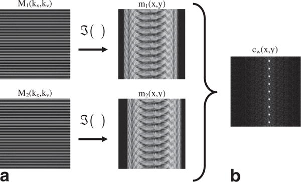
Shown in (a) are repeated, subsampled acquisition of k-space (such as acquiring the same echotrain twice) and the corresponding aliased images. The phase correlation, c_w(x,y) shown in (b) is obtained from the cross correlation of the aliased images. The crosscorrelation shows the replicated delta functions offset from the zero-offset position.

This correlation can be expressed in convolution integral as:

$$c_L(x,y)=\underset{-\infty }{\overset{\infty }{{\displaystyle \int }}}{c}_w(x,y-y\prime )e^{\frac{i\mathrm{\pi }y\prime }{N\mathrm{\Delta }y}(2L-N+N_{et})}\frac{\sin (\mathrm{\pi }y\prime /\mathrm{\Delta }y)}{\sin (\mathrm{\pi }y\prime /N_e\mathrm{\Delta }y)}dy\prime$$ [8]

where Δy is the spacing between voxels. After some algebra this becomes:

$$c_L(x,y)={\displaystyle \sum }_{j=0}^{N_{et}-1}{N}_e{e}^{i\mathrm{\pi }(\frac{2L}{N_{et}}+N_e-1)j}{C}_W(x,y-j{N}_e\mathrm{\Delta }y).$$ [9]

Thus, c_w(x,y) is replicated with spacing N_eΔy (the number of echoes in each echotrain times the voxel spacing) with a phase that depends on the shift (L) of the k-space measurements. If the motion in the y-direction (y_L) occurring between two acquisitions of the same subset (Lth echotrain acquired twice) is smaller than the aliasing distance:

$$Y_L<\left|\frac{N_e\mathrm{\Delta }y}{2}\right|$$ [10]

then two repeated subsets (echotrains) rather than two samplings of full k-space can be used to detect the motion of the object.

Correlation of Adjacent Lines

In this work, we carry this observation one step further to show that it is possible to detect motion between two adjacent sets of k-space measurements. Suppose an image is reconstructed using equally spaced measurements from a single echotrain with all other measurements set to zero. In that case, a highly aliased version of the original image is obtained, as shown in Figure 2a. Interestingly, a second image reconstructed from an adjacent set of equally spaced lines in k-space has some similarity to the first aliased image (Fig. 2b). If the object were to shift between acquisitions, one would expect that similar structures in both aliased images would also shift. In fact, one might naively assume that a crosscorrelation of these two aliased images could be used to determine the shift. Unfortunately crosscorrelation in image space corresponds to a multiplication in k-space. Because each echotrain is a different set of k-space lines, the multiplication in k-space is identically zero and no information about motion between the two aliased images is available. Instead, consider what happens if we physically shift each k-space line in the first echotrain by ½Δk_y and each line in the adjacent echotrain by −½Δk_y. If a crosscorrelation is then taken, the correlation function described in Eq. [3] is modified as:

$$\begin{array}{l}C\left(k_x,k_y+\frac{1}{2}\right)=|M_1(k_x,k_y)|\\ \cdot |M_1(k_x,k_y+1)|e^{i{\mathrm{\varphi }}_1(k_x,k_y)-i{\mathrm{\varphi }}_1(k_x,k_y+1)}{e}^{i\left(k_x{x}_L+\left(k_y+\frac{1}{2}\right)y_L\right)}\end{array}$$ [11]

where the phase function ϕ₁(k_x,k_y) = arg[M₁(k_x,k_y)] is the phase of each k-space point in the absence of any motion. The weighted correlation function becomes:

$$\begin{array}{l}{C}_w\left(k_x,k_y+\frac{1}{2}\right)\\ =e^{i-\arg \left[C\left(k_x,k_y+\frac{1}{2}\right)\right]}=e^{i\left(k_x{x}_L+\left(k_y+\frac{1}{2}\right)y_L\right)+i{\mathrm{\varphi }}_{\mathrm{Err}}(k_x,k_y)}\end{array}$$ [12]

where ϕ_Err(k_x,k_y) = ϕ₁(k_x,k_y) − ϕ₁(k_x,k_y +1) is the phase error term and is caused by the fact that adjacent k-space lines are not perfectly correlated.

FIG. 2.

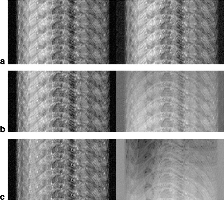
2D TSE hand images reconstructed from a single echotrain (N_e = 17 and N_et = 31). The images correspond to three adjacent sets of equally spaced k-space lines from the (a) 15th, (b) 16th, and (c) 17th echotrains. The left side is the magnitude image and the right side is the real image. The real image shows the slow variation in phase caused by the shift in the k-space sampling pattern.

If an object fills less than the measured FOV in the phase-encoding direction (i.e., an extended FOV is acquired), then it can be shown that there is at least some correlation between adjacent measurements in k-space. An object having a finite region of support is equivalent to multiplication by a rectangular window in image space, or convolution with a sinc-function in k-space. The width of the sinc-function in k-space is inversely related to the width of the image support. Therefore, as the measured FOV increases and the sinc-function broadens, the correlation between adjacent k-space lines increases and the phase error term is reduced. In practice, we will use a finite FOV, so there will always be some residual phase error. The transform of the correlation function will still contain a delta function offset from the origin by x_L and y_L, but will now be convolved with an error term due to ϕ_Err(k_x,k_y).

$$C_w(x,y)=\delta (x-x_L,y-y_L)\otimes \mathfrak{J}(e^{i{\mathrm{\varphi }}_{\mathrm{Err}}})$$ [13]

Any linear component of the phase error term will cause a shift in the delta function and will directly affect the accuracy of the motion estimates. The higher order terms of the phase error tend to blur and distort the delta function, making it difficult to accurately locate the delta peak.

To the extent that the phase error term is small, it is then possible to detect the motion between adjacent groups of lines of k-space. By using this technique to measure the incremental motion between every pair of adjacent echotrains, the complete motion history during a scan can be obtained. The absolute position of the object at the time of each echotrain is obtained by adding the shifts:

$$x_{\mathit{Shift}}(t)={\displaystyle {\sum }_{L=1}^t{x}_L}$$ [14]

and the same for the y direction. This motion history can then be used to correct a TSE MRI acquisition for nonrotational rigid-body motion. Motion correction is accomplished by applying the appropriate linear phase shift for each echotrain. It is shown in the following sections that a reasonable FOV can be selected such that the phase error is small enough to produce motion-corrected images.

METHODS

Ten data sets of 2D TSE head images were obtained on a Siemens Trio 3T MRI scanner from a volunteer using a single-channel head coil. Each data set was acquired at a different FOV but imaging parameters were selected to keep resolution, SNR, and contrast as constant as possible across all data sets (Table 1). Five different slice locations were acquired in each data set. Each image has a resolution of 0.5 mm × 0.5 mm × 2 mm, pulse repetition time (TR) = 3 s, echo time (TE) = 13 ms, and 11 echoes per echotrain.

Table 1.

Imaging Parameters Used to Acquire 2D TSE Head Images

Samples	FOV	% FOV (PE Direction)	BW/Pixel
418 × 418	209 mm2	105	130
462 × 462	231 mm2	116	144
506 × 506	253 mm2	126	157
550 × 550	275 mm2	138	172
594 × 594	297 mm2	149	183
638 × 638	319 mm2	160	196
682 × 682	341 mm2	171	209
726 × 726	363 mm2	182	222
770 × 770	385 mm2	193	241
814 ×814	407 mm2	204	256

FOV = field of view; SNR = signal-to-noise ratio. TR = pluse repetition time; TE = echo time; ETL = extract, transform, load. Parameters were selected to hold the resolution, SNR, and contrast constant, while allowing for a variable FOV in the phase encoding direction. Five interleaved slices were acquired with a 0.5 mm × 0.5 mm 2 mm resolution, ETL = 11, TR = 3 s, and TE = 13 ms.

Motion artifacts were introduced by applying varying linear phase shifts to each echotrain taking into account the slice interleaving and phase encoding order used to acquire the images. The amount of motion between two successive echotrains was randomly selected with the maximum value constrained to satisfy Eq. [10]. For the rotation experiments, the object was rotated (postacquisition) back and forth by a fixed value between each echotrain.

To test the algorithm in conjunction with actual motion, 11 high-resolution 2D TSE images of a human hand were acquired on a Siemens Trio 3T MRI scanner using a single-channel wrist coil. The images were acquired with a TR/TE = 4000/60 ms, extract, transform, load (ETL) (N_e) = 17 and 31 echotrains (N_et). The acquisition FOV = 120 mm, slice thickness = 3 mm, N_aqx = 640, N_aqy = 527, giving a spatial resolution of 0.1875 mm and 0.2277 mm in the x and y, respectively. The hand filled about one-third of the imaged FOV. During the acquisition, the subject moved his hand occasionally.

All human studies were approved by the institutional review board and informed consent was obtained from the volunteers.

RESULTS

The motion detected for the TSE head images with a FOV twice the object size is shown in Figure 3. The solid line in Figure 3a and b shows the actual motion applied to the head images, whereas the dots represent the motion calculated using the self-navigating technique proposed in this work. It has been assumed that the typical motion of an object will follow some relatively smooth time course. This smooth time course was accomplished by multiplying the Fourier Transform of the detected objects motion in time by a low-pass filter. The error between this band-limited curve and the actual motion is shown in Figure 3c. For this TSE data set, the maximum error is less than 0.4 mm in either direction.

FIG. 3.

Simulated motion tracking on TSE head images with an FOV double the object size, five interleaved slices with a 0.5 mm × 0.5 mm 2 mm resolution, ETL = 11, TR = 3 s, and TE = 13 ms. The top graphs show motion detection in the (a) readout or x direction, and (b) phase encode or y direction. The gray dots represent the motion calculated using self-navigation, and the solid line is the actual motion. The Fourier transform of the calculated data is multiplied by a low-pass filter to produce a smoothed line for the objects motion. A smoothed line is then fit to the calculated data and compared to the actual motion in (c). The solid line is the error in the x (readout) direction, whereas the dashed line is error in the y (phase encode) direction.

The images obtained from these motion estimates are shown in Figure 4. Each of the five columns represent one of the five acquired slice locations. Figure 4c shows the corrected images when no band-limited curve is fit to the data (i.e., motion represented by the dots in Fig. 3a, b). Although the images offer a significant improvement over the motion-corrupted images (Fig. 4b), there is still some unwanted motion artifact. This residual artifact is reduced when the motion is constrained to be band-limited (Fig. 4d).

FIG. 4.

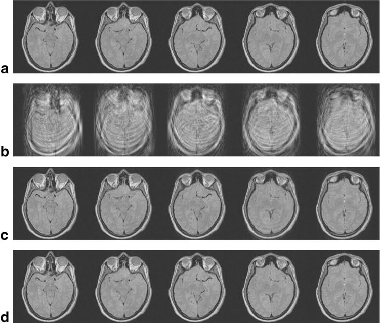
TSE head images acquired with the parameters in Table 1 and the motion correction shown in Figure 3. Each vertical column represents a different slice location. The images without motion artifacts are shown in (a), the motion corrupted images in (b), images corrected individually in (c), and with constrained motion using all five slices in (d).

The effect of varying the FOV on motion artifact reduction is demonstrated in Figure 5. When the FOV approaches the size of the object, the self-navigating technique is not able to fully correct the motion artifacts (Fig. 5a). However, if we acquire a FOV of 126% the object size (Fig. 5c), many of the motion artifacts are eliminated. With a larger FOV of 171% the object size almost all the motion artifacts have been removed. This is supported when one looks at the coefficient of variation of the motion corrected images compared with the original motion free images as shown in Figure 6. Images obtained at a FOV of 126% have a coefficient of variation that is half the value for images obtained at a FOV of 100% the object size. For data sets with a FOV larger than 171% (the object size) the improvement continues but at a slower rate.

FIG. 5.

TSE motion corrected head images with varying FOV. The top row contains images corrected using the proposed self-navigating technique and the bottom row shows the difference images (compared to the original motion free image). Each column represents a different FOV with (a) 105%, (b) 116%, (c) 126%, (d) 138%, (e) 149%, (f) 160%, and (g) 171% of the objects region of support.

FIG. 6.

Coefficient of variation with the original motion free images for varying FOV. The dot-dashed line compares the uncorrected images, the solid line represents corrected images with a 2° degree rotation between echotrains, the dashed line is corrected images with a 1° rotation between echotrains, and the dotted line is corrected images with no object rotation during acquisition.

The ability to accurately detect motion with minor rotations is shown in Figures 6 and 7. The goal is not to correct for the rotation artifacts, but simply to show that the motion artifacts themselves can be corrected in the presence of small rotations. For both the 126% and 171% FOV data sets, it is shown that if the rotation of the object is less than two degrees between successive echotrains in a slice, the motion correction is still successful (Fig. 7.). Even when the roation is two degrees between each echotrain in a slice, there is still a reduction to the motion artifacts using the self-navigation technique, just to a lesser extent (Fig. 6).

FIG. 7.

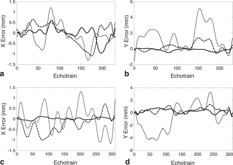
Error in motion correction using the proposed self-navigation technique in the presence of small object rotations. The top row shows the (a) X motion error and (b) Y motion error when the FOV is 126% the object size. The bottom row shows the (c) X motion error and (d) Y motion error when the FOV is 171% the object size. The solid lines represent no object rotation, the dashed line is a 1° rotation between any two adjacent data sets and the dotted line is a 2° rotation between any two adjacent data sets.

An image of the hand with occasional motion during the acquisition is shown in Figure 8a. The aliased images reconstructed from echotrains 15, 16, and 17 out of 31 are shown in Figure 2

FIG. 8.

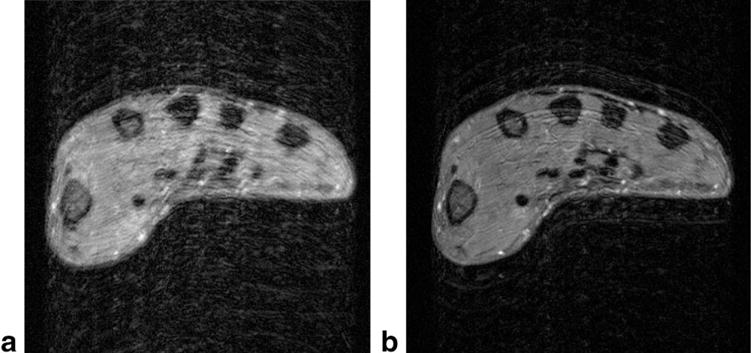
a: A single axial slice from a 22-slice T2w TSE images of the hand. Motion that occurred during acquisition caused severe blurring and some ghosting. b: An image obtained from the same measurement data of the same slice using the correction method described in this work.

For comparison, the image after correction using the technique of this work is shown in Figrue 8b. Nine of the 11 slices of the acquisition contained signal and similar results were observed in each of these. Because the slices are acquired in an interleaved fashion, one would expect the measured shift in each image to follow some relatively smooth time course. In Figure 9, the thick line plots the shift in the “y” direction for the nine slices in chronological order. It can be seen that the shifts are relatively smooth, as expected, and show nine movements in the negative direction. Also plotted in Figure 9 is the corresponding shift in the “x” direction (thin line).

FIG. 9.

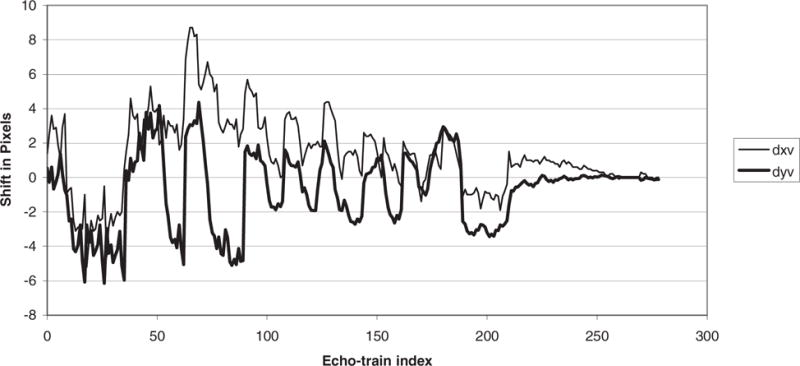
A plot of the x and y offsets in chronological order for 9 of the 11 interleaved slices where the SNR was strong enough for the correlation technique to be applied.

DISCUSSION

It has been demonstrated that MRI data can be self-navigating under the circumstances that subsets of k-space measurements are acquired closely enough in time to limit motion and rotation between successive acquisitions, and that a FOV be selected such that adjacent subsets of measurements have an adequate amount of correlation.

The technique differs with the technique presented by Kadah et al. (31) where floating navigators encode motion in the phase encoding direction with one navigator at one k-space offset position. That offset position is a compromise to maintain a high enough SNR while avoiding aliasing in the measurement of any motion. On the other hand, this self-navigator technique spreads the measurements across k-space, allowing a small window in which the motion can be uniquely determined. The technique of Kadah et al (31) also has a small window in which the phase can be determined uniquely: $\mathrm{\phi }=\frac{{\mathrm{\phi }}_0\pm 2n\mathrm{\pi }}{2\mathrm{\pi }{k}_f}$ where k_f is the FNAV frequency offset from 0 and n is a positive integer.

Although it has been shown that self-navigation can be applied successfully, a few questions remain as to the limitations of the technique. First, the effect of the echotrain length has not been fully studied. We note that this method applies nicely to T2w TSE data where an echotrain length of at least 11 was used. However, the technique can also apply to acquisition orders with shorter echotrains if motion between adjacent and/or sequential echotrains is very small. Shorter echotrains would be generally used for T₁-weighted studies. Additionally, if motion is minimal between two sequentially acquired echotrains, it is possible to acquire the data from both trains such that when combined they form one set of equally spaced lines in k-space. Self-navigation can then be applied by testing for motion between sets of combined echotrains that are adjacent in k-space. Thus, one combined echotrain may be correlated with an adjacent combined echotrain.

Second, the effects of surface coils are not known. For example, when using an array of surface coils, the image support for each coil will be defined by the coil sensitivity, reducing the requirement for phase encoding oversampling.

Finally, self-navigation could work for nonuniform sampling of k-space and rather than finding the delta-function location in image space, it would be possible to fit the phase surface with an inclined plane.

We note that this technique should work also for multi-shot echo-planar imaging (EPI), GRASE pulse sequences, and any sequence where the order of acquisition allows minimal motion within the set, but the probability of motion is great between sets. It should be possible to configure the acquisition of most gradient echo sequences such that equally spaced sets of k-space are acquired in close temporal proximity such that motion between the set of lines is minimal, and motion between adjacent sets can be detected by correlation.

Although we did not discuss correcting rotations, there are at least two extensions of this method that could allow small rotations to be detected and corrected. First, we have performed experiments showing that the correlation in the phase encoding direction can be performed as a function of position in the readout direction. The slope of the correlation as a function of “x” indicates the magnitude of rotation. Experiments to verify this observation are ongoing. Second, the use of arrays of surface coils provides many opportunities for spatial localized sensitivities for individual coil measurements. The distribution of translations observed for each local coil can then be combined to provide an estimate of the translation and rotation of the rigid body. It is entirely possible that these local coil motion measurements may allow nonrigid-body motions to be estimated and ultimately corrected.

CONCLUSIONS

This work provides a demonstration that rigid-body translational motion that occurs during the acquisition of MRI data can be detected, quantified, and corrected using self-navigation when subsets of k-space measurements are acquired closely spaced in time such that motion occurs between subsets, and that there is sufficient support external to the object in the acquisition space that adjacent subsets of measurements are correlated.

References

- 1.Hennig J, Nauerth A, Friedburg H. RARE imaging: a fast imaging method for clinical MR. Magn Reson Med. 1986;3:823–833. doi: 10.1002/mrm.1910030602. [DOI] [PubMed] [Google Scholar]
- 2.Mulkern RV, Wong ST, Winalski C, Jolesz FA. Contrast manipulation and artifact assessment of 2D and 3D RARE sequences. Magn Reson Imaging. 1990;8:557–566. doi: 10.1016/0730-725x(90)90132-l. [DOI] [PubMed] [Google Scholar]
- 3.Constable RT, Anderson AW, Zhong J, Gore JC. Factors influencing contrast in fast spin-echo MR imaging. Magn Reson Imaging. 1992;10:497–511. doi: 10.1016/0730-725x(92)90001-g. [DOI] [PubMed] [Google Scholar]
- 4.Constable RT, Gore JC. The loss of small objects in variable TE imaging: implications for FSE, RARE, and EPI. Magn Reson Med. 1992;28:9–24. doi: 10.1002/mrm.1910280103. [DOI] [PubMed] [Google Scholar]
- 5.Le Roux P, Hinks RS. Stabilization of echo amplitudes in FSE sequences. Magn Reson Med. 1993;30:183–190. doi: 10.1002/mrm.1910300206. [DOI] [PubMed] [Google Scholar]
- 6.Ehman RL, Felmlee JP. Adaptive technique for high-definition MR imaging of moving structures. Radiology. 1989;173:255–263. doi: 10.1148/radiology.173.1.2781017. [DOI] [PubMed] [Google Scholar]
- 7.Butts K, de Crespigny A, Pauly JM, Moseley M. Diffusion-weighted interleaved echo-planar imaging with a pair of orthogonal navigator echoes. Magn Reson Med. 1996;35:763–770. doi: 10.1002/mrm.1910350518. [DOI] [PubMed] [Google Scholar]
- 8.Danias PG, McConnell MV, Khasgiwala VC, Chuang ML, Edelman RR, Manning WJ. Prospective navigator correction of image position for coronary MR angiography. Radiology. 1997;203:733–736. doi: 10.1148/radiology.203.3.9169696. [DOI] [PubMed] [Google Scholar]
- 9.de Crespigny AJ, Marks MP, Enzmann DR, Moseley ME. Navigated diffusion imaging of normal and ischemic human brain. Magn Reson Med. 1995;33:720–728. doi: 10.1002/mrm.1910330518. [DOI] [PubMed] [Google Scholar]
- 10.Hu X, Kim SG. Reduction of signal fluctuation in functional MRI using navigator echoes. Magn Reson Med. 1994;31:495–503. doi: 10.1002/mrm.1910310505. [DOI] [PubMed] [Google Scholar]
- 11.Kyriakos WE, Panych LP, Zientara GP, Jolesz FA. Implementation of a reduced field-of-view method for dynamic MR imaging using navigator echoes. J Magn Reson Imaging. 1997;7:376–381. doi: 10.1002/jmri.1880070221. [DOI] [PubMed] [Google Scholar]
- 12.McConnell MV, Khasgiwala VC, Savord BJ, Chen MH, Chuang ML, Edelman RR, Manning WJ. Prospective adaptive navigator correction for breath-hold MR coronary angiography. Magn Reson Med. 1997;37:148–152. doi: 10.1002/mrm.1910370121. [DOI] [PubMed] [Google Scholar]
- 13.Taylor AM, Jhooti P, Wiesmann F, Keegan J, Firmin DN, Pennell DJ. MR navigator-echo monitoring of temporal changes in diaphragm position: implications for MR coronary angiography. J Magn Reson Imaging. 1997;7:629–636. doi: 10.1002/jmri.1880070404. [DOI] [PubMed] [Google Scholar]
- 14.Tyszka JM, Silverman JM. Navigated single-voxel proton spectroscopy of the human liver. Magn Reson Med. 1998;39:1–5. doi: 10.1002/mrm.1910390102. [DOI] [PubMed] [Google Scholar]
- 15.Wang Y, Rossman PJ, Grimm RC, Riederer SJ, Ehman RL. Navigator-echo-based real-time respiratory gating and triggering for reduction of respiration effects in three-dimensional coronary MR angiography. Radiology. 1996;198:55–60. doi: 10.1148/radiology.198.1.8539406. [DOI] [PubMed] [Google Scholar]
- 16.Wirestam R, Salford LG, Thomsen C, Brockstedt S, Persson BR, Stahlberg F. Quantification of low-velocity motion using a navigator-echo supported MR velocity-mapping technique: application to intracranial dynamics in volunteers and patients with brain tumours. Magn Reson Imaging. 1997;15:1–11. doi: 10.1016/s0730-725x(96)00341-4. [DOI] [PubMed] [Google Scholar]
- 17.Sachs TS, Meyer CH, Irarrazabal P, Hu BS, Nishimura DG, Macovski A. The diminishing variance algorithm for real-time reduction of motion artifacts in MRI. Magn Reson Med. 1995;34:412–422. doi: 10.1002/mrm.1910340319. [DOI] [PubMed] [Google Scholar]
- 18.Crowe L, Keegan J, Gatehouse P, Mohiaddhin R, Varghese A, Symmonds K, Cannell T, Yang GZ, Firmin D. Improvement of 3D volume selective turbo spin echo imaging for carotid artery wall imaging with navigator detection of swallowing. J Cardiovasc Magn Reson. 2005;7:203–205. doi: 10.1002/jmri.20424. [DOI] [PubMed] [Google Scholar]
- 19.Anderson AW, Gore JC. Analysis and correction of motion artifacts in diffusion weighted imaging. Magn Reson Med. 1994;32:379–387. doi: 10.1002/mrm.1910320313. [DOI] [PubMed] [Google Scholar]
- 20.Ordidge RJ, Helpern JA, Qing ZX, Knight RA, Nagesh V. Correction of motional artifacts in diffusion-weighted MR images using navigator echoes. Magn Reson Imaging. 1994;12:455–460. doi: 10.1016/0730-725x(94)92539-9. [DOI] [PubMed] [Google Scholar]
- 21.Wang Y, Ehman RL. Retrospective adaptive motion correction for navigator-gated 3D coronary MR angiography. J Magn Reson Imaging. 2000;11:208–214. doi: 10.1002/(sici)1522-2586(200002)11:2<208::aid-jmri20>3.0.co;2-9. [DOI] [PubMed] [Google Scholar]
- 22.Welch EB, Manduca A, Grimm RC, Ward HA, Jack CR., Jr Spherical navigator echoes for full 3D rigid body motion measurement in MRI. Magn Reson Med. 2002;47:32–41. doi: 10.1002/mrm.10012. [DOI] [PubMed] [Google Scholar]
- 23.Fu ZW, Wang Y, Grimm RC, Rossman PJ, Felmlee JP, Riederer SJ, Ehman RL. Orbital navigator echoes for motion measurements in magnetic resonance imaging. Magn Reson Med. 1995;34:746–753. doi: 10.1002/mrm.1910340514. [DOI] [PubMed] [Google Scholar]
- 24.Li D, Kaushikkar S, Haacke EM, Woodard PK, Dhawale PJ, Kroeker RM, Laub G, Kuginuki Y, Gutierrez FR. Coronary arteries: three-dimensional MR imaging with retrospective respiratory gating. Radiology. 1996;201:857–863. doi: 10.1148/radiology.201.3.8939242. [DOI] [PubMed] [Google Scholar]
- 25.Pipe JG. Motion correction with PROPELLER MRI: application to head motion and free-breathing cardiac imaging. Magn Reson Med. 1999;42:963–969. doi: 10.1002/(sici)1522-2594(199911)42:5<963::aid-mrm17>3.0.co;2-l. [DOI] [PubMed] [Google Scholar]
- 26.Larkman DJ, Atkinson D, Hajnal JV. Artifact reduction using parallel imaging methods. Top Magn Reson Imaging. 2004;15:267–275. doi: 10.1097/01.rmr.0000143782.39690.8a. [DOI] [PubMed] [Google Scholar]
- 27.Bydder M, Larkman DJ, Hajnal JV. Detection and elimination of motion artifacts by regeneration of k-space. Magn Reson Med. 2002;47:677–686. doi: 10.1002/mrm.10093. [DOI] [PubMed] [Google Scholar]
- 28.Pruessmann KP, Weiger M, Scheidegger MB, Boesiger P. SENSE: sensitivity encoding for fast MRI. Magn Reson Med. 1999;42:952–962. [PubMed] [Google Scholar]
- 29.Sodickson DK, Manning WJ. Simultaneous acquisition of spatial harmonics (SMASH): fast imaging with radiofrequency coil arrays. Magn Reson Med. 1997;38:591–603. doi: 10.1002/mrm.1910380414. [DOI] [PubMed] [Google Scholar]
- 30.Bydder M, Larkman DJ, Hajnal JV. Generalized SMASH imaging. Magn Reson Med. 2002;47:160–170. doi: 10.1002/mrm.10044. [DOI] [PubMed] [Google Scholar]
- 31.Kadah YM, Abaza AA, Fahmy AS, Youssef AB, Heberlein K, Hu XP. Floating navigator echo (FNAV) for in-plane 2D translational motion estimation. Magn Reson Med. 2004;51:403–407. doi: 10.1002/mrm.10704. [DOI] [PubMed] [Google Scholar]