

Abstract
The goal of association mapping is to identify genetic variants that predict disease, and as the field of human genetics matures, the number of successful association studies is increasing. Many such studies have shown that for many diseases, risk is explained by a reasonably large number of variants that each explains a very small amount of disease risk. This is prompting the use of genetic risk scores in building predictive models, where information across several variants is combined for predictive modeling. In the current study, we compare the performance of four previously proposed genetic risk score methods and present a new method for constructing genetic risk score that incorporates explained variance information. The methods compared include: a simple count Genetic Risk Score, an odds ratio weighted Genetic Risk Score, a direct logistic regression Genetic Risk Score, a polygenic Genetic Risk Score, and the new explained variance weighted Genetic Risk Score. We compare the methods using a wide range of simulations in two steps, with a range of the number of deleterious single nucleotide polymorphisms (SNPs) explaining disease risk, genetic modes, baseline penetrances, sample sizes, relative risks (RR) and minor allele frequencies (MAF). Several measures of model performance were compared including overall power, C-statistic and Akaike’s Information Criterion. Our results show the relative performance of methods differs significantly, with the new explained variance weighted GRS (EV-GRS) generally performing favorably to the other methods.
Keywords: explained variance, polygenic, predictive modeling, simple count genetic risk score, weighted genetic risk score
1 INTRODUCTION
An important priority in the area of genetic epidemiology is the identification of susceptible variants for the common disease. These genetic variants could further be incorporated in a feasible model to predict the disease risk, so that the environmental or therapeutic interventions could be introduced earlier to prevent the diseases or improve personalized treatment. In recent years, Genome-Wide Association Studies (GWAS) and candidate polymorphism investigations have identified a large number of variants that are consistently associated with the risk of complex diseases (Manolio 2010). However, most of the currently identified genetic variants convey a relatively modest effect, and the predictive value is limited. Anticipating the discovery of a large number of novel genetic variants in the near future, we need to prepare an appropriate framework to translate the emerging genomic knowledge into clinical utility, including the construction of genetic risk scores, the measurement of the predictive value, and the validation of the prediction models (Janssens and van Duijn 2009).
To address these issues, many analytical methods and models have been developed to better predict the disease risk using these low-effect risk variants. Recent studies have suggested possible risk models incorporating previously consistent genetic and conventional (clinical, demographic, etc.) risk factors (Meigs, et al. 2008; Talmud, et al. 2010). These genetic variants are included on the basis of consistent GWAS signals or meta-analysis results of association studies (De Jager, et al. 2009; Talmud, et al. 2010; Taylor, et al. 2011). Such improvements have had mixed results in predicting the risk of several common diseases, such as Type II diabetes (Meigs, et al. 2008; Talmud, et al. 2010), multiple sclerosis (De Jager, et al. 2009), systemic lupus erythematosus (Taylor, et al. 2011), breast cancer (Zheng, et al. 2010), lung cancer (Young, et al. 2009) and cardiovascular diseases (Paynter, et al. 2010), etc. Among these models, unweighted and weighted genetic risk score functions were used to construct genetic risk score profiles (De Jager, et al. 2009; Karlson, et al. 2010; Lin, et al. 2009; Meigs, et al. 2008; Paynter, et al. 2010; Seddon, et al. 2009; Talmud, et al. 2010; Taylor, et al. 2011; Young, et al. 2009; Zheng, et al. 2010). While these approaches have shown anecdotal success in real data analyses, these risk score functions have not been rigorously evaluated and compared. The assessment and comparison of the statistical properties of these functions in a range of scenarios is crucial for the proper application and interpretation of these methods.
In the current study, we try to compare the performance of four previously proposed methods: a simple count Genetic Risk Score (SC-GRS) (Talmud, et al. 2010), an odds ratio weighted Genetic Risk Score (OR-GRS) (De Jager, et al. 2009; Karlson, et al. 2010; Talmud, et al. 2010), a direct logistic regression Genetic Risk Score (DL-GRS) (Carayol, et al. 2010) and a polygenic Genetic Risk Score (PG-GRS) (Carayol, et al. 2010), and present a new method using an explained variance weighted Genetic Risk Score (EV-GRS). In a two-step simulation study, we used a wide range of simulated genetic models with a range of the number of deleterious single nucleotide polymorphisms (SNPs) in the etiology of disease risk, genetic modes, baseline penetrances, sample sizes, relative risks (RR) and minor allele frequencies (MAF) of the SNPs. We applied the risk score methods to the simulated data, and compared their performance based on power, C-statistic and Akaike’s Information Criteria (AIC) metrics.
2 METHODS
2.1 EXISTING GENETIC RISK SCORE MODELS
To simplify the analysis, we assume that one SNP per susceptibility gene has been selected, assuming these SNPs are uncorrelated and in turn contribute to the disease in an additive way. As described above, a very simple model is assumed. Let D denote the disease status where D = 1 if the subject has the disease (case) and D = 0 if healthy (control). Let G denote a vector of all genotype combinations and Gi denote the number of risk alleles of the subject at i-th SNP. We assume all genotypes are available for all SNPs and individuals and therefore no data is missing. All parameters are estimated by fitting the logistic regression model (Carayol, et al. 2010; Cordell and Clayton 2002).
2.1.1 Simple count GRS (SC-GRS)
| (1) |
| (2) |
This simple count model involves only two parameters. The risk score profile utilized the sum of all risk alleles for all SNPs. No prior information about the effect size of associated SNP is required. It is relatively simple and thus has a wide application for current research, especially when current literature is insufficient to provide stable estimates for each SNP’s effect (Paynter, et al. 2010). However, the presumed assumption of equal contributions of all SNPs may not be plausible.
2.1.2 Odds ratio weighted GRS (OR-GRS)
| (3) |
| (4) |
| (5) |
| (6) |
This model also needs two parameters. Here, the unequal effect size of SNPs is taken into account. The risk score is constructed as the weighted sum of all SNPs. The wOR is a pre-determined fixed weight. Practically, it is usually the log per-allele OR from meta-analysis for this SNP (Talmud, et al. 2010). It is easy to derive that SNP(s) with larger OR tends to contribute more to disease risk. This method requires external determinants, but in some cases they are unavailable if no studies were done before or inaccurate prior determinants were provided. This requirement makes this type of risk score unavailable for some studies, where previous estimates are not available. To make the weighted genetic risk score more directly comparable to the simple count genetic risk score, we used the rescaled version of the OR-GRS by multiplying by the rescaling factor .
2.1.3 Direct logistic regression GRS (DL-GRS)
| (7) |
| (8) |
This alternative weighted method directly fits a logistic regression model. The risk coefficient is the log(OR) for SNP i using the original dataset. The number of risk alleles is counted and multiplied by the risk coefficient to derive the risk score. No external information (i.e. an effect estimate from previous studies) is needed but I+1 parameters are estimated (Carayol, et al. 2010). Because this score is developed from the data at hand, the question of external validation inevitably arises. It can be assumed that if this score is applied in independent data, its fit will be substantially worse than the fit when applied in the first data in which it was built. The underlying goal of this risk score is essentially the same as with the OR-GRS, except that it is applied when external estimates of effect size are not available.
2.1.4 Polygenic GRS (PG-GRS)
| (9) |
| (10) |
For the PG model, two dummy variables are considered per SNP. Let xi1 be an indicator function of homozygous status and xi2 be an indicator of homozygous for risk allele at SNP i. Suppose a is the risk allele. Then, genotype AA is coded as 00, Aa as 10 and aa as 01. If we set AA as the baseline genotype, β1 is the risk coefficient for Aa and β2 is the risk coefficient for aa. In this aspect, the PG model is more flexible if the underlying genetic mode is unknown. The other methods discussed above make an additive genetic model assumption in adding the number of risk alleles. This assumption of additivity will decrease performance if there is dominance deviation in the actual underlying risk etiologies. While the ability to not be limited to genetic assumptions is appealing, the clear drawback is that the number of parameters 2I+1 is dramatically increasing as usually many SNPs were involved in reality (Carayol, et al. 2010). Additionally, as with the DL-GRS, this GRS relied exclusively on information derived from the original dataset, so the same concerns about external validation hold here.
2.2 NEW GENETIC RISK SCORE MODEL
2.2.1 Explained variance weighted GRS (EV-GRS)
| (11) |
| (12) |
| (13) |
| (14) |
Motivated by the effect size definition by Park and colleagues (Park, et al. 2010), we propose a new weighted method incorporating both OR and minor allele frequency (MAF) for SNP i, where the MAF estimate could be obtained from http://www.ncbi.nlm.nih.gov/projects/SNP/ or from published data, and OR estimate comes from the log per-allele odds ratio from external meta-analysis results. For individual SNP, we believe both OR and MAF are reasonable factors to define the explained variance and in turn to construct the prior contribution to the disease risk. It is expected that within the same OR, the disease risk will increase with increases of the MAF. This motivation is linked to the idea of Bayesian methods that we have already obtained priori knowledge of these variants and we could make use of the knowledge to improve our prediction. Similarly, the rescaled version of EV-GRS was used to make the genetic risk score more comparable to SC- and OR-GRS.
2.3 TWO-STEP SIMULATION DESIGN
We evaluated and tested the GRS methods in a two-step simulation study. In Step one, methods were compared for general performance in a range of simulations with similar minor allele frequencies and relative risks (in which case our EV-GRS method is equivalent to previous methods), and the relative performance of each approach was demonstrated. In Step two, methods that performed well in the first step of analysis and that have comparable numbers of parameters, and our new EV-GRS method are compared in a range of simulations where minor allele frequencies vary.
2.3.1 Step one simulation
Our primary goal in the Step 1 simulation was to detect general differences in performance among the four current genetic risk score models in a range of genetic models.
Factors of interest in the simulations included: the number of deleterious single nucleotide polymorphisms (SNP) that convey disease risk, the minor allele frequencies (MAF) of those SNPs, the relative risks (RR) of the associations, the underlying genetic modes, and the sample sizes of the datasets. We consider true disease risk models involving 2 and 6 deleterious SNPs, assuming Hardy-Weinberg Equilibrium (HWE). To simplify, we assume these SNPs contribute to the disease in an additive way with no interaction, and assume no linkage disequilibrium between them. We understand that these simplifications limit dissection of how these models perform in some cases, but do make the simulations manageable within the scope of the current study. Minor allele frequencies (MAF) for the SNPs were set to either 0.25 or 0.5 to represent common variants. Relative risks (RR) considered for our model were 1.5, 2 and 3 for 2 SNPs combination and 1.25, 1.5 and 1.75 for 6 SNPs combination (Figure 1). This range varies since high relative risks could lead to disease prevalence out of bounds for the large number of SNPs. This scenario represented realistic situations that the small number of causal variants with larger effect may lead to susceptibility to common diseases, while large number of variants influencing diseases usually may convey minor effects. The baseline penetrance was fixed at 0.1 to ensure a realistic population prevalence rate for common, complex diseases.
Figure 1.
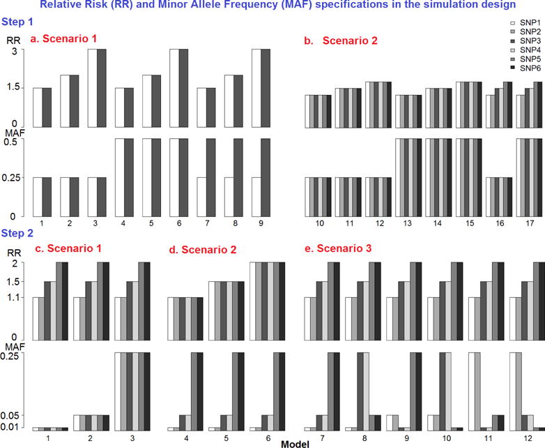
Relative risk and minor allele frequency specifications in the simulation design.
Simulated models are represented as penetrance functions. Penetrance functions define the probability of disease given a particular genotype combination at the disease risk locus. Penetrance functions under three genetic modes (recessive, additive and dominant modes) were explicitly determined, and the summary measures of effect size were calculated as described previously (Culverhouse, et al. 2002). Table 1 illustrates the two-locus penetrance patterns used in the current study as an example, where k was the baseline penetrance and θ was defined as the specified relative risk of having a disease between different genotypes for each SNP. Using a similar strategy, 6 SNP combinations models were also generated (details not shown). Balanced (equal allocation) case-control data was simulated with a total sample size of 250 and 500.
Table 1.
Penetrance patterns under three genetic modes for 2-locus main effect model.
| Mode | Genotype | BB | Bb | bb | ||
|---|---|---|---|---|---|---|
| Recessive | AA | k | k | θbk | ||
| Aa | k | k | θbk | |||
| aa | θak | θak | (θa+θb–1)k | |||
| Additive | AA | k |
|
θbk | ||
| Aa |
|
|
|
|||
| aa | θak |
|
(θa + θb −1)k | |||
| Dominant | AA | k | θbk | θbk | ||
| Aa | θak | (θa +θb −1)k | (θa + θb −1)k | |||
| aa | θak | (θa +θb −1)k | (θa + θb −1)k |
All combinations of MAF, RR, genetic modes, and sample sizes were generated, resulting in a total of 102 models in Step 1 simulation study (detailed in Appendix Table 1). For each model, 100 replicate datasets were simulated. Since only models 7–9 represent different MAF and models 16–17 represent different RR settings, the new EV-GRS method was not applied here.
2.3.2 Step two simulation
After analyzing the results from Step 1, we decided to choose SC- and OR-GRS (which perform better than the other approaches, as discussed in the results) and compared them to our new explained variance weighted GRS. These three methods include only 2 parameters in the statistical model and it is fair to compare them in respect of same number of parameters (and degrees of freedom). In this step, the impacts of RR and MAF were our primary interests, and the specific values chosen are detailed in Appendix Table 2. Three scenarios of interest are considered, including scenario 1 with different RR and same MAF, scenario 2 with same RR and different MAF, and scenario 3 with different RR and different MAF. The scenario with both the same RR and same MAF was considered in Step 1 of the simulations study and thus not included in Step 2.
A total of six risk SNPs were simulated to allow for a wide range for both RR and MAF to be varied across the simulated models. A range of MAF for the risk models was simulated, including 0.01, 0.05 and 0.25, while RR ranges from 1.1, 1.5 to 2 (Figure 1). The impact of varying sample size was extensively investigated, and datasets were simulated with a wide range of sample sizes, ranging from small (100, 200 and 300) to large (400, 500 and 600). Additionally, sample sizes of 250, 700, 800, 900 and 1000 were evaluated, and the results and conclusions were similar to those discussed below (details not included). The baseline penetrance was also varied (0.01 and 0.1). Since the PG-GRS method was not applied to the Step 2 simulations, only additive genetic modes are considered. All combinations of these factors were simulated, resulting in 144 models for Step two simulations. For each model, 100 replicate datasets were simulated.
For both steps of the simulation, datasets were generated using R software (www.r-project.org). A summary of the models simulated in Steps 1 and 2 is shown in Figure 1.
2.4 PERFORMANCE MEASUREMENT
The performance of the genetic risk score methods was measured through power, C-statistic (area under curves) and AIC.
2.4.1 Power
The main focus of our analysis is to find the best method to predict disease status. Since we generated the datasets using pre-defined settings, the “true” model was known. For this simulation study, power was defined as the number of times the model was statistically significant at P-value<0.05 across the 100 replicates (Motsinger-Reif, et al. 2008). We used the likelihood ratio test as global measures of model fit. Higher power value indicates better overall performance of the method to detect the risk models using disease-predicting SNPs.
2.4.2 C-statistic (Area under the curve)
Receiver Operating Characteristic (ROC) analysis was performed such that the true positive rate (sensitivity) is plotted in function of the false positive rate (1-specificity) for different cut-off points. The C-statistic, that is area under ROC curves (AUC), was used to estimate the discriminatory capability of each model to distinguish case subjects from control subjects. This statistic is commonly used for model comparison from the perspective of predictive performance, and we compared the performance of each of the methods using this summary. The larger the C-statistic, the higher the overall accuracy of the model (Janssens and van Duijn 2009).
2.4.3 Akaike information criterion (AIC)
The Akaike information criterion is a measure of the goodness of fit of a statistical model with fewest free parameters. It provides a tool for comparison among different models where the model with minimum AIC value is preferred.
| (15) |
Where L is maximized likelihood function for the estimated model and I is the number of independently adjusted parameters in the model.
2.5 DATA ANALYSIS
All 100 replicates for all models were analyzed by the current four methods: SC-GRS, OR-GRS, DL-GRS and PG-GRS in Step 1, and SC-GRS, OR-GRS, EV-GRS in Step 2. For SC-GRS, we construct individual risk score profile by counting the number of risk alleles associated with disease. For OR-GRS, to mimic the process of using an estimate from previous meta-analyses, we combine 100 datasets for each model and average the log OR for i-th SNP to generate the weight used in the OR-GRS. For DL-GRS, we use internal weights (from the dataset being analyzed) for each individual SNP. For the PG-GRS, we use two dummy variables for each SNP to indicate the three possible genotypes. For the EV-GRS, we use the same log OR as used in the OR-GRS. Similarly, we combine 100 datasets for each model and estimate the risk allele frequency for i-th SNP as our estimate of the MAF. In practice, the MAF estimate could alternatively refer to external sources such as http://www.ncbi.nlm.nih.gov/projects/SNP/, or http://hapmap.ncbi.nlm.nih.gov/.
Because several of these genetic risk scores incorporate external estimates of the effect sizes of risk SNPs, we incorporated errors in these estimates into the analysis of the Step 2 simulations. While ideally external weight would be well-estimated, we recognize that this may not always be the case, and we did not want to be over-optimistic about the performance of the methods that use these external weights by only assuming accurate estimates. In this analysis, we considered three types of misspecification for the external estimates used to construct the weights: random, overestimated and underestimated. In the random misspecifications, for SNP i, a random error ei was generated using a uniform distribution ranging from −0.2 to 0.2. The weight with random error for SNP i was calculated as wi(1+ei), where wi is the correct weight. The overestimate and underestimate weights were calculated as wi ± 0.5 SD(wi), where the variance of the weight estimate was taken into account here. To make the weighted genetic risk score more comparable to unweighted risk score, the rescaled versions were used for all OR- and EV-GRS.
Logistic regression modeling was used to fit these data sets using each of the GRS methods, and C statistics, AIC and P-value for likelihood ratio test were recorded. For each model, C statistics and AIC were averaged across the 100 replicates and power was calculated as the times a true model was identified (P-value less than 0.05) across 100 replicates. All the results were statistically evaluated for differences in performance under a general linear mixed model and pair-wise contrasts between methods, similarly to the approach described previously (Winham, et al. 2010). Each model was treated as an observation, while the final results for power, C and AIC as response variables separately. In Step 1, RR, MAF, genetic modes, sample sizes and four methods were treated as fixed explanatory variables. In Step 2, RR, MAF, baseline penetrance, sample sizes and three methods were treated as fixed explanatory variables. For a given model, all methods were performed on the same dataset replicates, and therefore methods could be treated as repeated measurements on the same model. A random effect for model was included to account for this dependence. Analysis was performed separately for each scenario in Step 1 and Step 2. Tukey’s method was used to make all pairwise comparisons between methods. It is suitable for multiple comparisons since it controls for the experiment-wise error rate (Hsu 1996). These results allow us to identify which factors contribute to the response significantly and further whether or not these methods differ.
All data analyses were performed using SAS v9.2 software.
3 RESULTS
3.1 STEP ONE SIMULATION RESULTS
Appendix Tables 3 and 4 describe the details of the linear mixed model analysis of the analysis results for Step 1 of the simulation. All the simulation factors except the number of SNPs were incorporated into the mixed model. The results of the 2-SNP and 6-SNP models were analyzed separately. Because the trends are clear, details of the results can be found in the Appendix, and the results are summarized here.
First the significance of the simulation factors on the overall results was considered. Details of the analyses can be found in Appendix Tables 3 and 4 and Appendix Figures 1 through 6. The results show that genetic mode and MAF were not statistically significant factors for all three performance metrics (power, C and AIC). As expected, the sample size was a significant factor for each simulation scenario and performance metric except for the C-statistic in the 2 SNPs simulation scenarios. As expected, after accounting for other factors, the fixed effect of RR was statistically significant for all three performance metrics. For the models with the same MAF and RR, genetic mode was also a significant factor. As expected, the power, C and AIC continue to improve as relative risk increases across all simulations and methods.
Most importantly, to compare the results of the four GRS methods, pairwise comparisons were performed, for a total of six comparisons. Separating by the number of deleterious SNPs, SC- and OR-GRS do not differ significantly after adjusting for other simulation factors by all performance metrics, as shown in Appendix Table 5. DL- and PG-GRS differ significantly in terms of C and AIC but not in terms of power. In terms of C, PG-GRS is dramatically larger than DL-GRS and SC- and OR-GRS are smaller. In terms of AIC, these methods differ significantly in 6 SNPs scenarios (P-value<0.0001) but not in 2 SNPs scenarios. In addition, as presented in the simulation design Figure 1 a–b, two SNPs have different MAF settings (0.25 and 0.5) in models 7–9, while SNPs have different RR settings (1.25, 1.5 and 1.75) in models 16–17. Therefore the major difference between SC- and OR-GRS methods could be attributed to these models 7–9 (Appendix Figure 3) and models 16–17 (Appendix Figure 6). It is clear that OR-outperforms SC-GRS by all performance metrics, but the difference is significant only for C (P-value=0.0027) in models 7–9 (Appendix Table 6). Also, we compare SC- and OR-GRS by genetic modes. In models 7–9 with different MAF (Appendix Figure 3 a and d recessive modes), OR-GRS shows superior performance compared to SC-GRS in all performance metrics (larger power and C and smaller AIC). For dominant modes, C is higher for OR- than SC-GRS. No difference was detected between these two methods otherwise. In models 16–17 (different RR), 6 SNPs have different relative risk combinations varying from 1.25, 1.5 to 1.75. The performance of OR-GRS become more comparable to SC-GRS by all three performance metrics across all sample size and genetic modes (Appendix Figure 6), but the difference is not statistically significant (Appendix Table 6). In regards to the impact of MAF, the performance improves for recessive modes but decreases for dominant modes when MAF increases from 0.25 to 0.5 (Appendix Figure 6).
3.2 STEP TWO SIMULATION RESULTS
In Step 2, the results of the mixed model analysis indicated several important trends, and the most important results are summarized in Table 2. In this table, the results of pair-wise contrasts for each of the methods are shown, with significant differences indicated by the inclusion of the “best” method listed in the body of the table. The method with the significantly better performance for a particular performance metric is listed in the body of the table (P-value<0.05 for the difference). If no method is indicated, there is no significant difference. The details of the mixed model analysis, including results for the simulation factors themselves, are detailed in Appendix Table 7. The important trends from these analyses are discussed below. The mean performance metrics and the associated Tukey adjusted P-values were given in Appendix Tables 8 and 9 respectively.
Table 2.
Significant winner in pair-wise method comparisons on Power, C and AIC in Step 2 simulation (Significant winner denotes the method significantly outperforms in the pair-wise method comparisons with larger power and C, and smaller AIC, and Tukey adjusted P-value is smaller than 0.05. The blank means no significant difference was detected in this pair).
| Scenario | Weightd | Power | C | AIC | ||||||
|---|---|---|---|---|---|---|---|---|---|---|
| SC-OR | SC-EV | OR-EV | SC-OR | SC-EV | OR-EV | SC-OR | SC-EV | OR-EV | ||
| 1a | Correct | OR | EV | OR | EV | OR | EV | |||
| 100–600 | Random | OR | EV | OR | EV | OR | EV | |||
| Overestimate | OR | EV | OR | EV | OR | EV | ||||
| Underestimate | ||||||||||
| 2b | Correct | SC | EV | SC | EV | SC | EV | |||
| 100–300 | Random | SC | EV | SC | EV | SC | EV | |||
| Overestimate | SC | EV | SC | EV | SC | EV | ||||
| Underestimate | SC | SC | EV | SC | SC | EV | SC | SC | ||
| 2b | Correct | SC | OR | |||||||
| 400–600 | Random | SC | OR | |||||||
| Overestimate | SC | EV | SC | EV | SC | EV | ||||
| Underestimate | SC | EV | SC | SC | EV | SC | SC | EV | ||
| 3c | Correct | OR | EV | EV | EV | EV | OR | EV | EV | |
| 100–300 | Random | OR | EV | EV | EV | EV | OR | EV | EV | |
| Overestimate | SC | EV | EV | SC | EV | SC | EV | |||
| Underestimate | SC | SC | EV | SC | SC | EV | SC | SC | EV | |
| 3c | Correct | OR | EV | OR | EV | OR | EV | |||
| 400–600 | Random | OR | EV | OR | EV | OR | EV | |||
| Overestimate | OR | EV | OR | EV | EV | EV | ||||
| Underestimate | SC | EV | SC | SC | EV | SC | EV | |||
Scenario 1 is different RR and same MAF among 6 SNPs.
Scenario 2 is same RR and different MAF among 6 SNPs.
Scenario 3 is different RR and different MAF among 6 SNPs.
Four weight estimate methods for OR- and EV-GRS: correct, random, overestimate and underestimate.
These results demonstrate that both RR and MAF were significant simulation factors for all three performance measurement metrics (P-value<0.0001). The baseline penetrance of the simulated model was a significant factor for all performance metrics in both scenarios 1 and 3, and for the C metric in scenario 2 with small sample sizes, while it is important overall in the large sample sizes. Sample size was a significant factor for power and AIC, but not significant for C in most cases. Methods were significantly different in scenarios 1 and 3, and scenario 2 with small sample, but not for power and C in scenario 2 when the sample size was large.
The results for each of the methods for the simulation scenario 1 (different relative risks and same minor allele frequencies, baseline penetrance=0.1) for the sample size of 200 are shown in Figure 2. The trends for other sample sizes are similar, as detailed in Appendix Table 10. The results of the analyses for simulation scenario 2 for the sample size of 200 are shown in Figure 3, and the results from scenario 2 for the sample size of 500 are shown in Figure 4. The details of the results across all sample sizes are listed in Appendix Table 11. Similarly, the results of the analyses for simulation scenario 3 for the sample size of 200 are shown in Figure 5. Additionally, the results from scenario 3 for larger sample size of 500 are shown in Figure 6. The details of the results across all sample sizes are listed in Appendix Table 12. For each of these scenarios, the analysis was repeated with no error in the external weight estimate, random error in the weight estimate, and systematic over- or under-estimates in the external weight estimates, and the results are shown across these different conditions in each of the figures. Details of the results across all sample sizes and scenarios are listed in Appendix Tables 10–12.
Figure 2. Model comparisons in Step 2 Scenario 1.
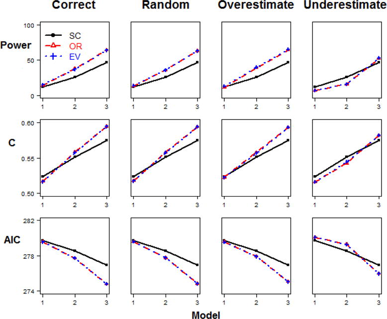
(different relative risk and same minor allele frequency, baseline penetrance=0.1, n=200).
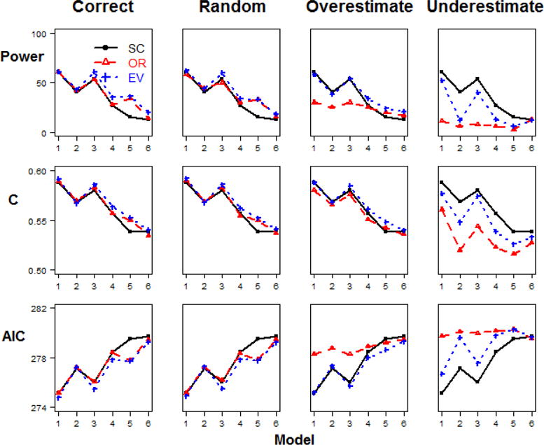
Figure 3. Model comparisons in Step 2 Scenario 2.
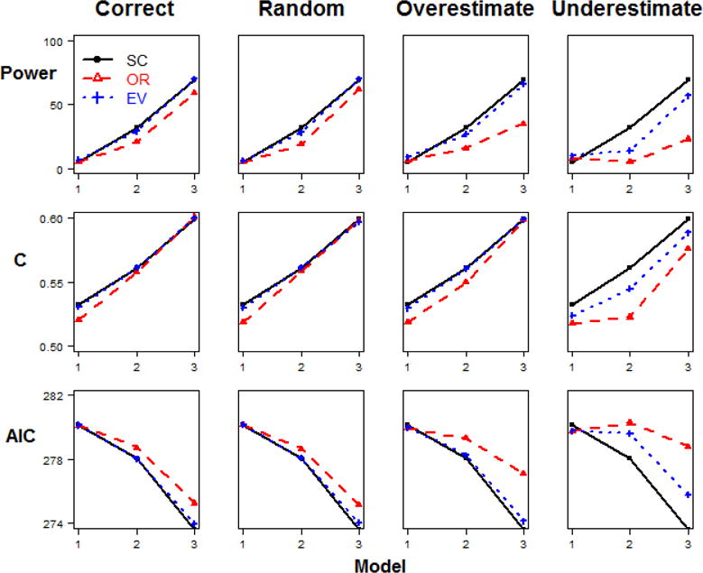
(same relative risk and different minor allele frequency, baseline penetrance=0.1, n=200).
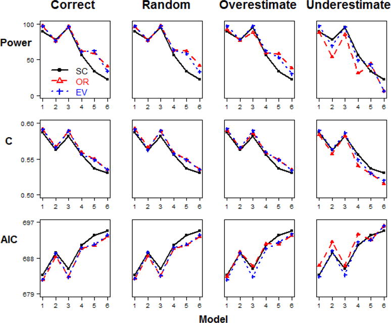
Figure 4. Model comparisons in Step 2 Scenario 2.
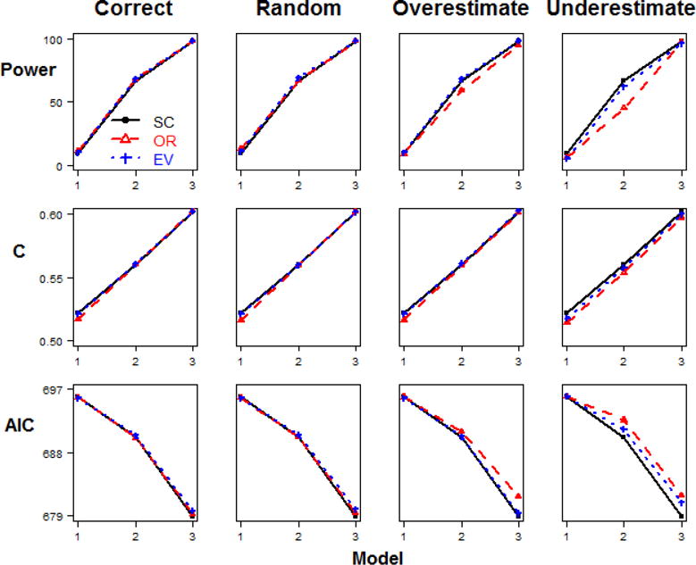
(same relative risk and different minor allele frequency, baseline penetrance=0.1, n=500).
Figure 5. Model comparisons in Step 2 Scenario 3.
(different relative risk and different minor allele frequency, baseline penetrance=0.1, n=200).
Figure 6. Model comparisons in Step 2 Scenario 3.
(different relative risk and different minor allele frequency, baseline penetrance=0.1, n=500).
In scenario 1, the 6 disease risk SNPs have different RR but the same MAF combination. In this case, with the same allele frequencies for each SNP, only OR matters in the weight, and hence OR- and EV-GRS are equivalent. In Figure 2 (scenario 1 with baseline penetrance=0.1 and sample size n=200), we observe that the weighted methods outperform the simple count method, but no difference is detected between OR- and EV-GRS (Table 2). This is true for the correct weight estimate case, as well as when weights had random or overestimated error. When the underestimated weight construction was used, there was no significant difference among all three methods by all performance metrics. In the case of different RR combinations among SNPs, weighted methods using OR significantly outperform the methods that do not use a weighted measure. As expected, with MAF or sample size increasing, the performance of all methods improves overall. In addition, it seems that the performance improves sharply when MAF changes from 0.01 to 0.05, while the improvement speed decreases from 0.05 to 0.25. This pattern was consistent for all baseline penetrance and sample size, and the detailed results were given in Appendix Table 10.
In scenario 2, the 6 disease-risk SNPs have the same RR but different MAF. When the sample size is relatively small (Figure 3), SC- and EV-GRS outperform OR-GRS significantly (Table 2), for correct, random and overestimated weights. No significant difference was detected between SC- and EV-GRS. If the underestimated weight was applied instead, SC-GRS is the best overall and EV-GRS is still preferable than OR-GRS.
However, with large sample size and correct or random weight (Figure 4), no significant differences were detected among weighted and simple summary methods, except that AIC of the EV-GRS method is larger (Table 2). If the weight was overestimated, SC- and EV-GRS would be favorable (Table 2). If the weight was underestimated, SC-GRS would be the best choice and EV- is better than OR-GRS (Table 2). These results demonstrate that in the case of different MAF combinations among SNPs, a weighted method that incorporates allele frequency (EV-GRS) is consistently better than that only involves OR (OR-GRS). Also, the results show that the simple count method (SC-GRS) is preferable than OR-GRS.
Scenario 3 was meant to represent a more realistic complicated situation, where the SNPs involved have different RR and different MAF combinations. Our results show that in the case when the sample size is relatively small (Figure 5), our new weighted method (EV-GRS) outperforms the other methods using all three performance assessment metrics (Table 2). This is consistently true for correct, random and overestimated weights. For underestimated weights, SC-GRS is the best and EV- is better than OR-GRS.
When the sample size is large (Figure 6), it is clear that the weighted methods (OR- and EV-GRS) are significantly preferable than simple count method (SC-GRS) overall, but no significant difference was observed between two weighted methods (Table 2). This is true for correct, random and overestimated weights generally. For underestimated weight, SC- and EV-GRS are favorable.
4 DISCUSSION
In the current study, we evaluated the performance of four existing genetic risk score construction methods: a simple count Genetic Risk Score (SC-GRS), an odds ratio weighted Genetic Risk Score (OR-GRS), a direct logistic regression Genetic Risk Score (DL-GRS), a polygenic Genetic Risk Score (PG-GRS), and then introduced our new weighted method an explained variance weighted Genetic Risk Score (EV-GRS). Three performance metrics (power, C and AIC) were investigated in our data analysis. These risk score methods represent some commonly used approaches in the literature, but it is certainly not an exhaustive list of all genetic risk score models proposed. For instance, Lin et al. (2009) suggest a weighted genetic score using log lower bound odds ratio as weights, to penalize SNPs with less reliable OR estimates (Lin, et al. 2009), and future studies should consider a more comprehensive list of potential methods.
The results of the simulation experiments show several important trends. As expected, in general, sample size and relative risk are important simulation factors for all methods performance in our investigation. As sample size increases, the risk predication becomes more accurate. Similarly, as the relative risk becomes larger, the predication ability improves. However, in respect to the impacts of MAF and genetic mode as simulation factors, the trends are not so clear and straightforward, which merits further investigation. Step 2 results indicate the performance improves sharply when MAF increases for low effect sizes, and then the improvement speed decreases when MAF grows bigger. This pattern also corresponds to the assumption of explained variance (effect size) weight construction that MAF and odds ratio may dominate the overall direction of effect size. Further refinement of the effect estimate may be a promising future direction.
The primary interest of our study is to compare the relative performance of the GRS methods. Power (global model fit) is an important criterion for methods comparisons. In Step 1, SC- and OR-GRS have higher power than DL- and PG-GRS in most of cases, especially for 6 SNPs scenarios (though exceptions to this general trend do exist for some recessive modes). For instance, the power is nearly the same among SC-, OR- and PG-GRS (Appendix Figures 2–4). It is not surprising to observe PG-GRS has the highest C-statistic (discrimination) for all model types, since it has larger number of parameters and therefore better accuracy of discrimination. We also introduce AIC for further evaluation to penalize the large number of parameters. To illustrate the influence of the number of free parameters, 2 SNPs and 6 SNP disease-risk scenarios were simulated and evaluated. For the 2 SNPs scenarios, both SC- and OR-GRS have 2 fixed parameters, while DL-GRS has 3(I + 1) and PG-GRS has 5(2I + 1) parameters. The difference among the number of parameters is large enough for the sample sizes generated (representing realistic sample sizes in genetic studies) to separate the performance for all model types. Therefore, PG-GRS has higher AIC (worse performance) than other methods in many cases. For 6 SNPs scenarios, the number of parameters of SC- and OR-GRS remains constant at 2, but DL-GRS has 7 and PG-GRS has 13 parameters. Consistently, the AIC of DL- and PG-GRS are larger than SC- and OR-GRS for all model types, since they were given more penalization. Therefore, for DL- and PG-GRS methods, as the number of SNPs involved in the profile or the corresponding free parameters increases, the influence on the AIC increases dramatically and therefore the performance decreases. In contrast, SC- and OR-GRS methods are not influenced by the number of SNPs involved in terms of AIC. In real data analysis, the number of SNPs used for genetic risk profile is likely to be large, and even much larger than 6 SNPs in our example. From this perspective, SC- and OR-GRS are preferred than DL- and PG-GRS methods.
Since SC- and OR-GRS methods are clearly preferred in terms of power and AIC, we then compare these two methods under scenarios 1–3 (different MAF among SNPs) and 2–3 (different RR). Our results indicate that the OR-GRS method outperforms the SC-GRS.
To further investigate these two methods of interest and the effect of MAF in the weight construction, we introduce explained variance weighted method and compare these three methods in Step 2 under scenarios with a wider range of RR and MAF settings. Results in scenario 1 with different RR indicate that the weighted methods are preferred to the simple count method when relative risks vary among SNPs. When MAF are the same, the odds ratio and explained variance weighted methods are equivalent. When the weight is underestimated, the three methods do not significantly differ (Table 2). Scenario 2 with different MAF is our primary interest to compare OR- and EV-GRS. In the case that all RR among SNPs are similar but the MAF vary greatly, the simple count and explained variance weighted methods significantly outperform the odds ratio weighted method (Table 2), when the sample size is relatively small with correct, random or overestimated weights (Figure 3). When the weights are underestimated, the SC-GRS is best. This is reasonable since in case of small sample sizes that estimates of the odds ratio may not be accurate and precise and it could introduce bias. Therefore, SC- or EV-GRS is preferred to the OR-GRS. When the sample size is large with correct or random weight, no significant differences were detected among three methods except that the AIC of the EV-GRS is large. In scenario 3, different RR and different MAF settings were simulated, and several trends were seen. When the sample size is small, the EV-GRS consistently yielded better performance than the OR-GRS. With large samples, the weighted methods significantly outperformed the simple count methods except in the case of underestimated weights.
In summary, the Step 2 results suggest that when MAF are similar but RR differ, OR- and EV-GRS are the best. When RR are similar but MAF vary, SC-and EV-GRS are preferred in case of small sample size. EV-GRS is unfavorable only in reference to the AIC in large sample sizes and no difference was observed among these three methods otherwise. When effect sizes (both MAF and RR) vary, OR- and EV-GRS are recommended in larger sample, and the EV-GRS is clearly the best in smaller sample size. This pattern is generally consistent if the weight is constructed correctly, or with error of small magnitude, or overestimated. However, if the weight is underestimated, SC-GRS is the best choice overall and EV-GRS is also a good alternative. Therefore, the performance of EV-GRS is fairly good and robust across the majority of situations simulated and the performance of weight construction, particularly for the more complex situations with relatively small sample sizes.
In conclusion, this study represents the first empirical comparison of genetic risk score models that have been anecdotally used in the literature, and provides some guidance for researchers in selecting a genetic risk score model under a series of different scenarios. The main points are outlined below. First, if the number of available SNPs involved in disease-risk is limited, and main goal of a study is discrimination ability between case and control status, the DL- or PG-GRS may be preferred. Second, when many SNPs were reported to contribute to the disease risk, and the importance of detecting and replicating risk models (power) is main focus, the SC- or the weighted GRS are preferred. Third, in real data analysis when the odds ratio estimates may not be available or may not be very reliable, the SC-GRS is an appropriate choice to avoid bias. The results from the SC-GRS in these situations may not differ drastically since many odds ratio estimates for SNPs are in small magnitude and may be similar across the disease-risk SNPs. Fourth, in another extreme, if previous study(s) provide decently reliable OR estimates and the estimates are very different across SNPs, the weighted GRS methods are preferable.
Lastly but most importantly, our study presents a new genetic risk score method, EV-GRS, that performs very well overall compared to previously introduced methods, both in extreme and general cases. The EV-GRS is highly recommended for several reasons. First, while there were a few situations where the EV-GRS was not clearly the best method, the EV-GRS was the most generally robust method. The EV-GRS should be applied as compared to the other methods so that AIC is not drastically lost when sample size is relatively large and power or discriminatory capability is maximized. It should also be noted that when we choose the odds ratio estimates from meta-analysis and combine the results across different studies, it is possible that different studies may have a wide range of sample and effect sizes. In this case, the OR- or SC-GRS methods may perform better slightly in some scenarios. Generally though, the EV-GRS is the best choice to be used across all scenarios. Second, with respect to the error of weight construction, we may not know whether the weight is correctly constructed or not in reality. The EV-GRS performs well when the weight is correct, or with some minor random error, or overestimated. Furthermore, its performance is still good compared with SC-GRS, even if the weight is underestimated. Without a priori knowledge of potential sample sizes and performance of weight construction, it is desirable to rely on a fairly robust method that tends to offer sufficient power and discriminatory capability for a variety of scenarios.
In considering the interpretation of the results of the simulation study, a few questions arose that we explored with smaller-scale simulation experiments, and include in the discussion here to frame the results of the current study. To test if the overall patterns were susceptible to the number of simulations used, we randomly picked one model and generated 500 replicates. As we did for the other simulations, the three methods (SC-, OR- and EV-GRS) were compared in terms of power, C-statistics and AIC, with different sources of error in constructing the weight (results not shown). The results show that running more simulations would give a very similar pattern to smaller simulation replicates, and the relative performance among these methods is still the same. Hence, the simulation with 100 replicates, which has been extensively applied in the current study, is sufficient to support our conclusion.
Due to the importance of validation in the discovery, development and validation of such risk score modeling, we also incorporated an independent validation step to simulations to obtain the external weight, using the similar strategy as above. One model was randomly replicated, and two weighted methods (OR- and EV-GRS) were compared. The SC-GRS does not require any external weight, and so we did not include it in this comparison. Moreover, we did not include the DL- and PG-GRS in the with-validation simulation because they could only apply the internal datasets for constructing the weights. Rather than using the internal weights (without-validation), another 100 independent datasets were generated to calculate the external weights (with-validation), with different sources of error. Results show that there is no significant difference in the performance metrics between with- and without-validation weights (results not shown). Furthermore, the pattern of relative performance is similar that leads to the same conclusion. Therefore, the without-validation weights could be sufficient to demonstrate the relative performance of these methods.
Understanding that the current simulations included simple genetic model, we also wanted to consider the case where there is dependency between SNPs. We considered true risk models involving two disease-causing SNPs (SNP1 and SNP2). We assume SNP1 is under Hardy-Weinberg Equilibrium (HWE), and there is linkage disequilibrium (LD) between SNP2 and SNP3. Two models are considered: (1) a genetic risk score model with the true disease-causing SNPs: SNP1+SNP2, and (2) a genetic risk score model with the true SNPs plus the additional SNP in LD: SNP1+SNP2+SNP3. Data were simulated under different settings of genotype frequencies and relative risks among these SNPs. We then evaluated the relative performance of the SC-, OR- and EV-GRS methods using these two different risk score formulations, to see if the methods were robust to such dependence between SNPs (data not shown). Consistently, the results show that SC-GRS performs much better under the true model (with only the disease-causing SNPs) than the model that includes the true SNPs plus additional SNP in LD, by all performance metrics. However, there was no significant difference for OR- and EV-GRS under these two models (with or without the third SNP in LD). Also, both the OR- and EV-GRS outperform SC-GRS, and these results strengthen the recommendation to use one of the weighted approaches. It is clear that SC-GRS may be sensitive to the true model. However, it is impractical to include the exact true causative SNPs in the risk model. More often, we may involve the potential “tagging” SNPs that may be in LD with the true disease-causing variants. It may be not of primary interest to dissect the “tagging” SNP from the true disease-causing SNPs for the purpose of prediction. In this case, weighted methods (OR- and EV-GRS) are more robust and preferable.
While the current extensive study shows the promise of the EV-GRS method, future studies should explore its performance in a broader range of realistic and complex scenarios, for example, with more true causal variants involved in the evaluation of the methods for both methodological comparisons and evaluations of the new EV-GRS model. In existing genetic risk models that have been built for human diseases, a wide range of the number of risk SNPs have been incorporated, such as 6 SNPs for age-related macular degeneration (Seddon, et al. 2009), 15 SNPs for Type 2 diabetes (Lin, et al. 2009), and 12 or 101 SNPs for cardiovascular disease (Paynter, et al. 2010). It seems that the number of SNPs involved in the risk model may depend on the disease etiology. Given this broad range, it is expected that incorporating a large number of SNPs into genetic risk models could be one of the important future directions. Apart from the genetic factors, clinical information could also be included in the prediction model, as a summary “clinical risk score” or a set of covariates, to make the application more practical. In the future, as the unparalleled development of technologies, more precise and stable effect size estimates for susceptibility SNPs will be obtained. Appropriate analytical strategies, combined with environmental risk factors and clinical information, will be imperative to predict the disease risk and to translate associations to clinical utility. More suitable and comprehensive weight construction strategies may be one of the solutions.
Acknowledgments
We would like to thank Howard McLeod for helpful discussions on risk score modeling, and the anonymous reviewers for comments and suggestions.
APPENDIX
Figure 1.
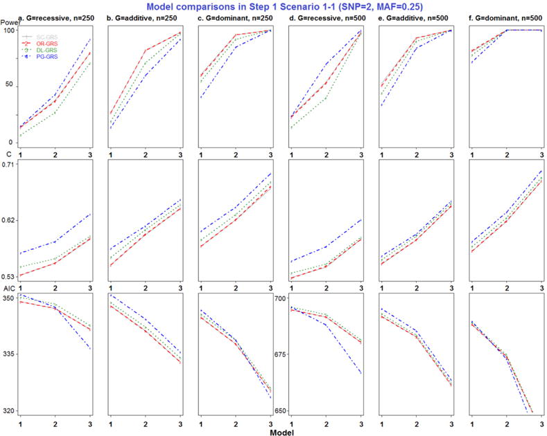
Model comparisons in Step 1 Scenario 1-1 (SNP=2, MAF=0.25).
Figure 2.
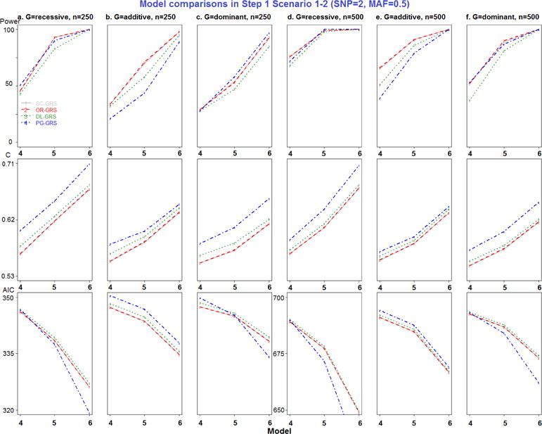
Model comparisons in Step 1 Scenario 1-2 (SNP=2, MAF=0.5).
Figure 3.
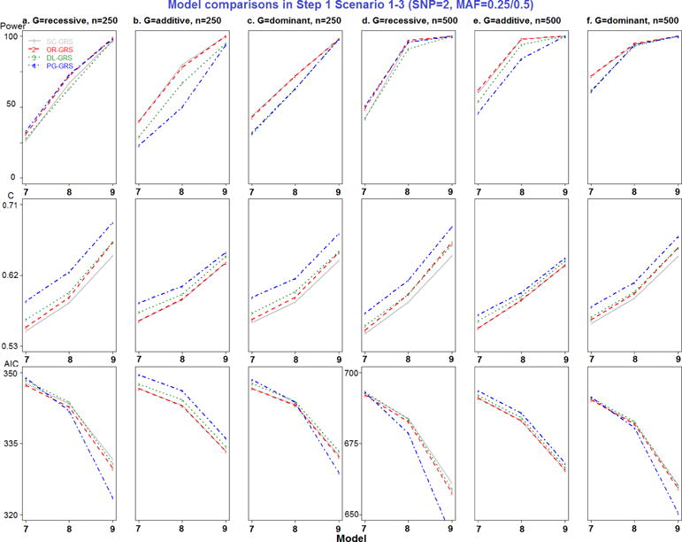
Model comparisons in Step 1 Scenario 1-3 (SNP=2, MAF=0.25/0.5).
Figure 4.
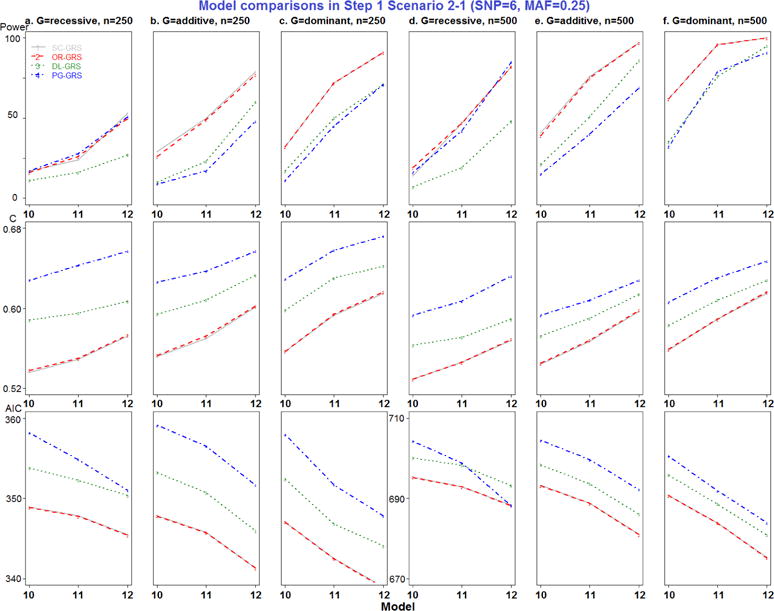
Model comparisons in Step 1 Scenario 2-1 (SNP=6, MAF=0.25).
Figure 5.
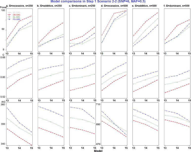
Model comparisons in Step 1 Scenario 2-2 (SNP=6, MAF=0.5).
Figure 6.
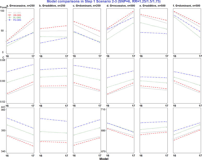
Model comparisons in Step 1 Scenario 2-3 (SNP=6, RR=1.25/1.5/1.75).
Table 1.
Relative Risk (RR) and Minor Allele Frequency (MAF) specifications in Step 1 simulation.
| Scenario | Model | RR | MAF | Prevalence | |||||
|---|---|---|---|---|---|---|---|---|---|
| 1/1–2a | 2/3–4b | 5–6 | 1/1–2a | 2/3–4b | 5–6 | ||||
| 1 (2SNPs) | 1-1 | 1 | 1.5 | 1.5 | 0.25 | 0.25 | 0.125 | ||
| 2 | 2 | 2 | 0.25 | 0.25 | 0.15 | ||||
| 3 | 3 | 3 | 0.25 | 0.25 | 0.2 | ||||
| 1-2 | 4 | 1.5 | 1.5 | 0.5 | 0.5 | 0.15 | |||
| 5 | 2 | 2 | 0.5 | 0.5 | 0.2 | ||||
| 6 | 3 | 3 | 0.5 | 0.5 | 0.3 | ||||
| 1-3 | 7 | 1.5 | 1.5 | 0.25 | 0.5 | 0.1375 | |||
| 8 | 2 | 2 | 0.25 | 0.5 | 0.175 | ||||
| 9 | 3 | 3 | 0.25 | 0.5 | 0.25 | ||||
| 2 (6 SNPs) | 2-1 | 10 | 1.25 | 1.25 | 1.25 | 0.25 | 0.25 | 0.25 | 0.1375 |
| 11 | 1.5 | 1.5 | 1.5 | 0.25 | 0.25 | 0.25 | 0.175 | ||
| 12 | 1.75 | 1.75 | 1.75 | 0.25 | 0.25 | 0.25 | 0.2125 | ||
| 2-2 | 13 | 1.25 | 1.25 | 1.25 | 0.5 | 0.5 | 0.5 | 0.175 | |
| 14 | 1.5 | 1.5 | 1.5 | 0.5 | 0.5 | 0.5 | 0.25 | ||
| 15 | 1.75 | 1.75 | 1.75 | 0.5 | 0.5 | 0.5 | 0.325 | ||
| 2-3 | 16 | 1.25 | 1.5 | 1.75 | 0.25 | 0.25 | 0.25 | 0.175 | |
| 17 | 1.25 | 1.5 | 1.75 | 0.5 | 0.5 | 0.5 | 0.25 | ||
1 denotes SNP1 for scenario 1 (2 disease-causing SNPs), and 1–2 denotes SNP1 and SNP2 for scenario 2 (6 disease-causing SNPs).
2 denotes SNP2 for scenario 1 (2 disease-causing SNPs), and 3–4 denotes SNP3 and SNP4 for scenario 2 (6 disease-causing SNPs).
Table 2.
Relative Risk (RR) and Minor Allele Frequency (MAF) specifications in Step 2 simulation.
| Scenario | Model | RR | MAF | Prevalenced | ||||
|---|---|---|---|---|---|---|---|---|
| 1–2 | 3–4 | 5–6 | 1–2 | 3–4 | 5–6 | |||
| 1a | 1 | 1.1 | 1.5 | 2 | 0.01 | 0.01 | 0.01 | 0.1032 |
| 2 | 1.1 | 1.5 | 2 | 0.05 | 0.05 | 0.05 | 0.116 | |
| 3 | 1.1 | 1.5 | 2 | 0.25 | 0.25 | 0.25 | 0.18 | |
| 2b | 4 | 1.1 | 1.1 | 1.1 | 0.01 | 0.05 | 0.25 | 0.1062 |
| 5 | 1.5 | 1.5 | 1.5 | 0.01 | 0.05 | 0.25 | 0.131 | |
| 6 | 2 | 2 | 2 | 0.01 | 0.05 | 0.25 | 0.162 | |
| 3c | 7 | 1.1 | 1.5 | 2 | 0.01 | 0.05 | 0.25 | 0.1552 |
| 8 | 1.1 | 1.5 | 2 | 0.01 | 0.25 | 0.05 | 0.1352 | |
| 9 | 1.1 | 1.5 | 2 | 0.05 | 0.01 | 0.25 | 0.152 | |
| 10 | 1.1 | 1.5 | 2 | 0.05 | 0.25 | 0.01 | 0.128 | |
| 11 | 1.1 | 1.5 | 2 | 0.25 | 0.01 | 0.05 | 0.116 | |
| 12 | 1.1 | 1.5 | 2 | 0.25 | 0.05 | 0.01 | 0.112 | |
Scenario 1 is different RR and same MAF among 6 SNPs.
Scenario 2 is same RR and different MAF among 6 SNPs.
Scenario 3 is different RR and different MAF among 6 SNPs.
Prevalence is based on the baseline penetrance 0.1.
Table 3.
P-values a of simulation factors on Power, C and AIC by 2 scenarios in Step 1 simulation.
| Effect | Scenario 1 (2 SNPs)
|
Scenario 2 (6 SNPs)
|
||||
|---|---|---|---|---|---|---|
| Power | C | AIC | Power | C | AIC | |
| RR | <.0001 | <.0001 | <.0001 | <.0001 | <.0001 | <.0001 |
| MAF | 0.4030 | 0.6824 | 0.9948 | 0.7168 | 0.8848 | 0.6516 |
| Genetic mode | 0.1639 | 0.2344 | 0.3627 | 0.6138 | 0.5871 | 0.5286 |
| Sample size | <.0001 | 0.4931 | <.0001 | <.0001 | 0.0008 | <.0001 |
| Method | <.0001 | <.0001 | 0.0025 | <.0001 | <.0001 | <.0001 |
P-values less than 0.05 are considered statistically significant.
Table 4.
P-values a of simulation factors on Power, C and AIC by each scenario in Step 1 simulation.
| Scenario | Effect | Scenario 1 (2 SNPs)
|
Scenario 2 (6 SNPs)
|
||||
|---|---|---|---|---|---|---|---|
| Power | C | AIC | Power | C | AIC | ||
| −1 | RR/MAF b | <.0001 | <.0001 | 0.0004 | <.0001 | <.0001 | <.0001 |
| Genetic mode | 0.0005 | <.0001 | 0.0130 | <.0001 | <.0001 | 0.0015 | |
| Sample size | 0.0305 | 0.3909 | <.0001 | 0.0002 | <.0001 | <.0001 | |
| Method | 0.0126 | <.0001 | 0.3377 | <.0001 | <.0001 | <.0001 | |
| −2 | RR/MAF b | <.0001 | <.0001 | <.0001 | <.0001 | <.0001 | 0.0001 |
| Genetic mode | 0.0113 | <.0001 | 0.0238 | 0.0014 | 0.0002 | 0.0095 | |
| Sample size | 0.0009 | 0.3698 | <.0001 | 0.0009 | 0.0004 | <.0001 | |
| Method | 0.0016 | <.0001 | 0.1049 | <.0001 | <.0001 | <.0001 | |
| −3 | RR/MAF b | <.0001 | <.0001 | <.0001 | 0.9229 | 0.8859 | 0.9318 |
| Genetic mode | 0.6006 | 0.0838 | 0.4973 | 0.9315 | 0.9136 | 0.8874 | |
| Sample size | 0.0004 | 0.3020 | <.0001 | 0.0642 | 0.2527 | <.0001 | |
| Method | 0.0002 | <.0001 | 0.1496 | <.0001 | <.0001 | <.0001 | |
P-values less than 0.05 are considered statistically significant.
RR/MAF denotes MAF effect only for scenarios 2–3 and RR otherwise.
Table 5.
Adjusted P-values a of pair-wise method comparisons on Power, C and AIC by 2 scenarios in Step 1 simulation.
| Method Comparisons | Scenario 1 (2 SNPs)
|
Scenario 2 (6 SNPs)
|
||||
|---|---|---|---|---|---|---|
| Power | C | AIC | Power | C | AIC | |
| SC—OR | 0.9841 | 0.0775 | 0.9781 | 0.6746 | 0.4668 | 0.6354 |
| SC—DL | <.0001 | <.0001 | 0.4213 | <.0001 | <.0001 | <.0001 |
| SC—PG | <.0001 | <.0001 | 0.1007 | <.0001 | <.0001 | <.0001 |
| OR—DL | <.0001 | <.0001 | 0.2187 | <.0001 | <.0001 | <.0001 |
| OR—PG | <.0001 | <.0001 | 0.2296 | <.0001 | <.0001 | <.0001 |
| DL—PG | 0.9471 | <.0001 | 0.001 | 0.9244 | <.0001 | <.0001 |
These P-values are adjusted by Tukey method and less than 0.05 are considered statistically significant.
Table 6.
Adjusted P-values a of pair-wise method comparisons on Power, C and AIC by each scenario in Step 1 simulation.
| Scenario | Method Comparisons | Scenario 1 (2 SNPs)
|
Scenario 2 (6 SNPs)
|
||||
|---|---|---|---|---|---|---|---|
| Power | C | AIC | Power | C | AIC | ||
| −1 | SC—OR | 0.9989 | 0.9900 | 1.0000 | 0.9992 | 0.9914 | 0.9995 |
| SC—DL | 0.0339 | 0.0003 | 0.5813 | <.0001 | <.0001 | <.0001 | |
| SC—PG | 0.1613 | <.0001 | 0.9603 | <.0001 | <.0001 | <.0001 | |
| OR—DL | 0.0485 | 0.0008 | 0.5738 | <.0001 | <.0001 | <.0001 | |
| OR—PG | 0.2118 | <.0001 | 0.963 | <.0001 | <.0001 | <.0001 | |
| DL—PG | 0.8981 | <.0001 | 0.2993 | 0.7850 | <.0001 | <.0001 | |
| −2 | SC—OR | 0.9992 | 0.9877 | 1.0000 | 1.0000 | 0.9872 | 0.9989 |
| SC—DL | 0.0147 | 0.0001 | 0.7805 | <.0001 | <.0001 | <.0001 | |
| SC—PG | 0.0563 | <.0001 | 0.4102 | <.0001 | <.0001 | <.0001 | |
| OR—DL | 0.0102 | 0.0003 | 0.7736 | <.0001 | <.0001 | <.0001 | |
| OR—PG | 0.0410 | <.0001 | 0.4173 | <.0001 | <.0001 | <.0001 | |
| DL—PG | 0.9520 | <.0001 | 0.071 | 0.9826 | <.0001 | <.0001 | |
| −3 | SC—OR | 0.8909 | 0.0027 | 0.9158 | 0.1127 | 0.1711 | 0.0861 |
| SC—DL | 0.0333 | <.0001 | 0.9631 | <.0001 | <.0001 | <.0001 | |
| SC—PG | 0.0118 | <.0001 | 0.3122 | <.0001 | <.0001 | <.0001 | |
| OR—DL | 0.0047 | 0.0229 | 0.6740 | <.0001 | <.0001 | <.0001 | |
| OR—PG | 0.0014 | <.0001 | 0.6937 | <.0001 | <.0001 | <.0001 | |
| DL—PG | 0.9792 | <.0001 | 0.1305 | 0.9910 | <.0001 | <.0001 | |
These P-values are adjusted by Tukey method and less than 0.05 are considered statistically significant.
Table 7.
P-values a of simulation factors on Power, C and AIC in Step 2 simulation (using correct weight).
| Scenario | Effect | Scenario −1c (100–300)
|
Scenario −2c (400–600)
|
||||
|---|---|---|---|---|---|---|---|
| Power | C | AIC | Power | C | AIC | ||
| 1 | RR/MAF b | <.0001 | <.0001 | <.0001 | |||
| Penetrance | 0.0165 | <.0001 | 0.0142 | ||||
| Sample size | <.0001 | 0.0704 | <.0001 | ||||
| Method | <.0001 | <.0001 | <.0001 | ||||
| 2 | RR/MAF b | <.0001 | <.0001 | 0.0001 | <.0001 | <.0001 | <.0001 |
| Penetrance | 0.4413 | 0.0260 | 0.3613 | 0.0398 | 0.0039 | 0.0362 | |
| Sample size | 0.0055 | 0.2784 | <.0001 | 0.0015 | 0.9165 | <.0001 | |
| Method | <.0001 | 0.0018 | 0.0003 | 0.3532 | 0.9384 | 0.0006 | |
| 3 | RR/MAF b | <.0001 | <.0001 | <.0001 | <.0001 | <.0001 | <.0001 |
| Penetrance | 0.0084 | <.0001 | 0.0088 | <.0001 | <.0001 | <.0001 | |
| Sample size | <.0001 | 0.0020 | <.0001 | <.0001 | 0.7237 | <.0001 | |
| Method | <.0001 | <.0001 | <.0001 | <.0001 | <.0001 | <.0001 | |
P-values less than 0.05 are considered statistically significant.
RR/MAF denotes MAF effect only for scenario 1, RR effect for scenario 2 and both RR and MAF effect for scenario 3.
For scenario 1, sample size is 100–600 and for scenarios 2 and 3, sample size is 100–300.
Table 8.
Mean of Power, C and AIC in Step 2 simulation.
| Scenario | Weight a | Power
|
C
|
AIC
|
||||||
|---|---|---|---|---|---|---|---|---|---|---|
| SC | OR | EV | SC | OR | EV | SC | OR | EV | ||
| 1 | Correct | 37.111 | 46.444 | 46.528 | 0.546 | 0.553 | 0.553 | 485.28 | 483.95 | 483.95 |
| 100–600 | Random | 46.083 | 46.056 | 0.552 | 0.552 | 484.01 | 484.01 | |||
| Overestimate | 44.333 | 44.778 | 0.552 | 0.553 | 484.15 | 484.13 | ||||
| Underestimate | 34.667 | 35.111 | 0.544 | 0.544 | 485.06 | 485.03 | ||||
| 2 | Correct | 32.778 | 28.278 | 31.889 | 0.562 | 0.558 | 0.562 | 277.71 | 278.08 | 277.78 |
| 100–300 | Random | 28.500 | 31.444 | 0.559 | 0.562 | 278.05 | 277.82 | |||
| Overestimate | 19.056 | 30.667 | 0.553 | 0.560 | 279 | 277.87 | ||||
| Underestimate | 9.611 | 21.056 | 0.533 | 0.547 | 279.83 | 278.9 | ||||
| 2 | Correct | 54.500 | 54.111 | 53.889 | 0.557 | 0.556 | 0.556 | 689.70 | 689.78 | 689.99 |
| 400–600 | Random | 54.333 | 53.722 | 0.556 | 0.556 | 689.84 | 690.07 | |||
| Overestimate | 49.389 | 54.222 | 0.555 | 0.557 | 690.69 | 689.83 | ||||
| Underestimate | 41.056 | 49.333 | 0.548 | 0.552 | 691.64 | 690.76 | ||||
| 3 | Correct | 31.778 | 34.639 | 37.611 | 0.562 | 0.562 | 0.566 | 277.92 | 277.64 | 277.38 |
| 100–300 | Random | 34.278 | 37.306 | 0.562 | 0.565 | 277.67 | 277.43 | |||
| Overestimate | 22.472 | 34.917 | 0.555 | 0.564 | 278.8 | 277.65 | ||||
| Underestimate | 10.75 | 21.444 | 0.533 | 0.548 | 279.79 | 278.87 | ||||
| 3 | Correct | 58.278 | 68.417 | 66.667 | 0.557 | 0.563 | 0.562 | 690.33 | 689 | 689.21 |
| 400–600 | Random | 68.222 | 66.222 | 0.562 | 0.561 | 689.1 | 689.31 | |||
| Overestimate | 63.111 | 65.694 | 0.561 | 0.562 | 690.02 | 689.31 | ||||
| Underestimate | 44.528 | 55.417 | 0.550 | 0.554 | 691.95 | 690.39 | ||||
Four weight estimate methods for OR and EV: correct, random, overestimate and underestimate.
Table 9.
Adjusted P-values a of pair-wise method comparisons on Power, C and AIC in Step 2 simulation.
| Power
|
C
|
AIC
|
||||||||
|---|---|---|---|---|---|---|---|---|---|---|
| Scenario | Weighta | SC-OR | SC-EV | OR-EV | SC-OR | SC-EV | OR-EV | SC-OR | SC-EV | OR-EV |
| 1 | Correct | <.0001 | <.0001 | 0.9943 | <.0001 | <.0001 | 0.9992 | <.0001 | <.0001 | 0.9999 |
| 100–600 | Random | <.0001 | <.0001 | 0.9993 | <.0001 | <.0001 | 0.9998 | <.0001 | <.0001 | 0.9997 |
| Over-est | <.0001 | <.0001 | 0.8645 | <.0001 | <.0001 | 0.9891 | <.0001 | <.0001 | 0.9876 | |
| Under-est | 0.1412 | 0.2657 | 0.9352 | 0.1554 | 0.2372 | 0.9708 | 0.4293 | 0.3570 | 0.9905 | |
| 2 | Correct | <.0001 | 0.6140 | 0.0014 | 0.0025 | 0.8339 | 0.0114 | 0.0004 | 0.6873 | 0.0038 |
| 100–300 | Random | <.0001 | 0.2776 | 0.0043 | 0.0022 | 0.7987 | 0.0119 | 0.0003 | 0.3532 | 0.0124 |
| Over-est | <.0001 | 0.6269 | <.0001 | <.0001 | 0.1932 | <.0001 | <.0001 | 0.7729 | 0.0002 | |
| Under-est | <.0001 | 0.0155 | 0.0185 | <.0001 | <.0001 | <.0001 | <.0001 | 0.0100 | 0.0510 | |
| 2 | Correct | 0.6310 | 0.3287 | 0.8590 | 0.9351 | 0.9691 | 0.9933 | 0.4783 | 0.0006 | 0.0137 |
| 400–600 | Random | 0.9462 | 0.3135 | 0.4835 | 0.533 | 0.3316 | 0.9306 | 0.1807 | <.0001 | 0.0090 |
| Over-est | 0.0008 | 0.9738 | 0.0015 | 0.0014 | 0.8099 | 0.0002 | 0.0001 | 0.8115 | 0.0008 | |
| Under-est | <.0001 | 0.1673 | 0.0145 | <.0001 | 0.0002 | <.0001 | <.0001 | 0.0046 | 0.0217 | |
| 3 | Correct | 0.0103 | <.0001 | 0.0074 | 0.8601 | <.0001 | <.0001 | 0.0028 | <.0001 | 0.0060 |
| 100–300 | Random | 0.0224 | <.0001 | 0.0044 | 0.7202 | <.0001 | 0.0003 | 0.0064 | <.0001 | 0.0110 |
| Over-est | <.0001 | 0.1595 | <.0001 | <.0001 | 0.1385 | <.0001 | <.0001 | 0.2138 | <.0001 | |
| Under-est | <.0001 | 0.0001 | <.0001 | <.0001 | <.0001 | <.0001 | <.0001 | 0.0001 | 0.0002 | |
| 3 | Correct | <.0001 | <.0001 | 0.3865 | <.0001 | <.0001 | 0.2557 | <.0001 | <.0001 | 0.1947 |
| 400–600 | Random | <.0001 | <.0001 | 0.2933 | <.0001 | <.0001 | 0.1219 | <.0001 | <.0001 | 0.1833 |
| Over-est | 0.0015 | <.0001 | 0.1328 | <.0001 | <.0001 | 0.3372 | 0.1408 | <.0001 | 0.0001 | |
| Under-est | <.0001 | 0.3666 | <.0001 | <.0001 | 0.0171 | <.0001 | <.0001 | 0.9713 | <.0001 | |
These P-values are adjusted by Tukey method and less than 0.05 are considered statistically significant.
Table 10-1.
Model specification in Step 2 scenario 1 simulation.
| Model Specification | |||||||
|---|---|---|---|---|---|---|---|
| Model | Type | OR1-2 | OR3-4 | OR5-6 | MAF1-6 | Penetrance | n |
| 1 | 1 | 1.1 | 1.5 | 2 | 0.01 | 0.1 | 100 |
| 2 | 2 | 1.1 | 1.5 | 2 | 0.05 | 0.1 | 100 |
| 3 | 3 | 1.1 | 1.5 | 2 | 0.25 | 0.1 | 100 |
| 4 | 1 | 1.1 | 1.5 | 2 | 0.01 | 0.1 | 200 |
| 5 | 2 | 1.1 | 1.5 | 2 | 0.05 | 0.1 | 200 |
| 6 | 3 | 1.1 | 1.5 | 2 | 0.25 | 0.1 | 200 |
| 7 | 1 | 1.1 | 1.5 | 2 | 0.01 | 0.1 | 300 |
| 8 | 2 | 1.1 | 1.5 | 2 | 0.05 | 0.1 | 300 |
| 9 | 3 | 1.1 | 1.5 | 2 | 0.25 | 0.1 | 300 |
| 10 | 1 | 1.1 | 1.5 | 2 | 0.01 | 0.1 | 400 |
| 11 | 2 | 1.1 | 1.5 | 2 | 0.05 | 0.1 | 400 |
| 12 | 3 | 1.1 | 1.5 | 2 | 0.25 | 0.1 | 400 |
| 13 | 1 | 1.1 | 1.5 | 2 | 0.01 | 0.1 | 500 |
| 14 | 2 | 1.1 | 1.5 | 2 | 0.05 | 0.1 | 500 |
| 15 | 3 | 1.1 | 1.5 | 2 | 0.25 | 0.1 | 500 |
| 16 | 1 | 1.1 | 1.5 | 2 | 0.01 | 0.1 | 600 |
| 17 | 2 | 1.1 | 1.5 | 2 | 0.05 | 0.1 | 600 |
| 18 | 3 | 1.1 | 1.5 | 2 | 0.25 | 0.1 | 600 |
| 19 | 1 | 1.1 | 1.5 | 2 | 0.01 | 0.01 | 100 |
| 20 | 2 | 1.1 | 1.5 | 2 | 0.05 | 0.01 | 100 |
| 21 | 3 | 1.1 | 1.5 | 2 | 0.25 | 0.01 | 100 |
| 22 | 1 | 1.1 | 1.5 | 2 | 0.01 | 0.01 | 200 |
| 23 | 2 | 1.1 | 1.5 | 2 | 0.05 | 0.01 | 200 |
| 24 | 3 | 1.1 | 1.5 | 2 | 0.25 | 0.01 | 200 |
| 25 | 1 | 1.1 | 1.5 | 2 | 0.01 | 0.01 | 300 |
| 26 | 2 | 1.1 | 1.5 | 2 | 0.05 | 0.01 | 300 |
| 27 | 3 | 1.1 | 1.5 | 2 | 0.25 | 0.01 | 300 |
| 28 | 1 | 1.1 | 1.5 | 2 | 0.01 | 0.01 | 400 |
| 29 | 2 | 1.1 | 1.5 | 2 | 0.05 | 0.01 | 400 |
| 30 | 3 | 1.1 | 1.5 | 2 | 0.25 | 0.01 | 400 |
| 31 | 1 | 1.1 | 1.5 | 2 | 0.01 | 0.01 | 500 |
| 32 | 2 | 1.1 | 1.5 | 2 | 0.05 | 0.01 | 500 |
| 33 | 3 | 1.1 | 1.5 | 2 | 0.25 | 0.01 | 500 |
| 34 | 1 | 1.1 | 1.5 | 2 | 0.01 | 0.01 | 600 |
| 35 | 2 | 1.1 | 1.5 | 2 | 0.05 | 0.01 | 600 |
| 36 | 3 | 1.1 | 1.5 | 2 | 0.25 | 0.01 | 600 |
Table 10-2.
Power in Step 2 scenario 1 simulation.
| Power | |||||||||
|---|---|---|---|---|---|---|---|---|---|
| Correct | Random | Overestimate | Underestimate | ||||||
| Model | SC | OR | EV | OR | EV | OR | EV | OR | EV |
| 1 | 8 | 13 | 14 | 14 | 14 | 8 | 7 | 8 | 8 |
| 2 | 13 | 19 | 19 | 19 | 18 | 14 | 15 | 10 | 10 |
| 3 | 32 | 39 | 38 | 41 | 41 | 35 | 35 | 16 | 15 |
| 4 | 12 | 14 | 15 | 13 | 14 | 11 | 13 | 7 | 7 |
| 5 | 26 | 38 | 37 | 36 | 36 | 39 | 40 | 16 | 16 |
| 6 | 47 | 64 | 64 | 63 | 63 | 64 | 65 | 52 | 53 |
| 7 | 5 | 15 | 15 | 15 | 15 | 11 | 11 | 3 | 3 |
| 8 | 36 | 50 | 50 | 49 | 49 | 46 | 46 | 24 | 27 |
| 9 | 66 | 84 | 84 | 83 | 83 | 85 | 85 | 78 | 78 |
| 10 | 14 | 17 | 17 | 17 | 18 | 19 | 19 | 7 | 8 |
| 11 | 55 | 69 | 70 | 69 | 69 | 66 | 67 | 58 | 58 |
| 12 | 82 | 96 | 96 | 95 | 95 | 92 | 92 | 95 | 95 |
| 13 | 23 | 24 | 24 | 26 | 26 | 26 | 26 | 6 | 6 |
| 14 | 56 | 70 | 71 | 71 | 71 | 72 | 73 | 65 | 66 |
| 15 | 93 | 98 | 98 | 98 | 98 | 98 | 98 | 97 | 97 |
| 16 | 21 | 25 | 24 | 25 | 25 | 25 | 25 | 5 | 5 |
| 17 | 72 | 82 | 83 | 83 | 82 | 79 | 80 | 74 | 75 |
| 18 | 87 | 97 | 97 | 98 | 98 | 97 | 97 | 96 | 96 |
| 19 | 12 | 12 | 12 | 12 | 12 | 10 | 10 | 8 | 9 |
| 20 | 16 | 19 | 17 | 17 | 16 | 12 | 13 | 5 | 5 |
| 21 | 15 | 23 | 23 | 22 | 22 | 22 | 22 | 7 | 7 |
| 22 | 8 | 15 | 15 | 14 | 14 | 13 | 13 | 4 | 5 |
| 23 | 25 | 33 | 33 | 33 | 32 | 28 | 31 | 2 | 3 |
| 24 | 35 | 51 | 51 | 50 | 50 | 45 | 45 | 39 | 39 |
| 25 | 10 | 9 | 9 | 7 | 7 | 13 | 13 | 11 | 11 |
| 26 | 27 | 36 | 36 | 34 | 34 | 30 | 34 | 18 | 18 |
| 27 | 46 | 64 | 64 | 64 | 64 | 62 | 62 | 52 | 53 |
| 28 | 17 | 17 | 19 | 16 | 17 | 14 | 15 | 10 | 9 |
| 29 | 42 | 49 | 49 | 51 | 51 | 44 | 45 | 40 | 43 |
| 30 | 59 | 80 | 80 | 77 | 77 | 80 | 79 | 73 | 73 |
| 31 | 14 | 23 | 23 | 22 | 22 | 18 | 19 | 2 | 2 |
| 32 | 47 | 59 | 60 | 60 | 60 | 56 | 56 | 41 | 43 |
| 33 | 67 | 84 | 84 | 81 | 81 | 77 | 77 | 74 | 74 |
| 34 | 17 | 21 | 21 | 21 | 21 | 23 | 22 | 4 | 5 |
| 35 | 56 | 70 | 70 | 71 | 71 | 72 | 72 | 57 | 57 |
| 36 | 75 | 92 | 92 | 92 | 92 | 90 | 90 | 84 | 85 |
Table 10-3.
C in Step 2 scenario 1 simulation.
| C | |||||||||
|---|---|---|---|---|---|---|---|---|---|
| Model | SC | Correct | Random | Overestimate | Underestimate | ||||
| OR | EV | OR | EV | OR | EV | OR | EV | ||
| 1 | 0.5289 | 0.5261 | 0.5256 | 0.5252 | 0.5251 | 0.5271 | 0.5272 | 0.5249 | 0.5249 |
| 2 | 0.5571 | 0.5618 | 0.5605 | 0.5618 | 0.5622 | 0.5600 | 0.5624 | 0.5462 | 0.5466 |
| 3 | 0.5813 | 0.5916 | 0.5915 | 0.5925 | 0.5923 | 0.5908 | 0.5925 | 0.5636 | 0.5631 |
| 4 | 0.5235 | 0.5167 | 0.5165 | 0.5174 | 0.5173 | 0.5225 | 0.5224 | 0.5161 | 0.5159 |
| 5 | 0.5516 | 0.5582 | 0.5579 | 0.5579 | 0.5576 | 0.5579 | 0.5566 | 0.5425 | 0.5445 |
| 6 | 0.5749 | 0.5947 | 0.5946 | 0.5942 | 0.5941 | 0.5933 | 0.5933 | 0.5818 | 0.5822 |
| 7 | 0.5175 | 0.5164 | 0.5164 | 0.5164 | 0.5163 | 0.5160 | 0.5160 | 0.5143 | 0.5143 |
| 8 | 0.5477 | 0.5566 | 0.5566 | 0.5559 | 0.5560 | 0.5545 | 0.5545 | 0.5400 | 0.5410 |
| 9 | 0.5750 | 0.5922 | 0.5921 | 0.5917 | 0.5917 | 0.5914 | 0.5915 | 0.5865 | 0.5866 |
| 10 | 0.5194 | 0.5203 | 0.5202 | 0.5202 | 0.5203 | 0.5194 | 0.5195 | 0.5151 | 0.5153 |
| 11 | 0.5516 | 0.5593 | 0.5594 | 0.5588 | 0.5589 | 0.5593 | 0.5595 | 0.5528 | 0.5532 |
| 12 | 0.5760 | 0.5940 | 0.5941 | 0.5932 | 0.5932 | 0.5929 | 0.5929 | 0.5905 | 0.5906 |
| 13 | 0.5169 | 0.5160 | 0.5161 | 0.5163 | 0.5162 | 0.5166 | 0.5164 | 0.5100 | 0.5100 |
| 14 | 0.5499 | 0.5582 | 0.5583 | 0.5583 | 0.5583 | 0.5577 | 0.5578 | 0.5491 | 0.5497 |
| 15 | 0.5764 | 0.5945 | 0.5946 | 0.5942 | 0.5942 | 0.5938 | 0.5939 | 0.5919 | 0.5919 |
| 16 | 0.5177 | 0.5161 | 0.5161 | 0.5162 | 0.5162 | 0.5179 | 0.5177 | 0.5046 | 0.5046 |
| 17 | 0.5498 | 0.5574 | 0.5575 | 0.5574 | 0.5574 | 0.5570 | 0.5571 | 0.5531 | 0.5530 |
| 18 | 0.5762 | 0.5937 | 0.5937 | 0.5931 | 0.5931 | 0.5930 | 0.5931 | 0.5912 | 0.5913 |
| 19 | 0.5308 | 0.5219 | 0.5224 | 0.5216 | 0.5214 | 0.5274 | 0.5274 | 0.5252 | 0.5262 |
| 20 | 0.5552 | 0.5563 | 0.5570 | 0.5558 | 0.5567 | 0.5515 | 0.5520 | 0.5416 | 0.5437 |
| 21 | 0.5687 | 0.5775 | 0.5775 | 0.5776 | 0.5777 | 0.5753 | 0.5759 | 0.5468 | 0.5472 |
| 22 | 0.5222 | 0.5200 | 0.5197 | 0.5213 | 0.5209 | 0.5209 | 0.5210 | 0.5161 | 0.5173 |
| 23 | 0.5484 | 0.5494 | 0.5504 | 0.5500 | 0.5494 | 0.5517 | 0.5515 | 0.5297 | 0.5300 |
| 24 | 0.5646 | 0.5801 | 0.5803 | 0.5785 | 0.5785 | 0.5781 | 0.5783 | 0.5658 | 0.5662 |
| 25 | 0.5186 | 0.5182 | 0.5182 | 0.5178 | 0.5178 | 0.5173 | 0.5173 | 0.5162 | 0.5161 |
| 26 | 0.5414 | 0.5466 | 0.5460 | 0.5455 | 0.5454 | 0.5459 | 0.5460 | 0.5274 | 0.5274 |
| 27 | 0.5629 | 0.5761 | 0.5761 | 0.5756 | 0.5756 | 0.5748 | 0.5750 | 0.5675 | 0.5676 |
| 28 | 0.5187 | 0.5160 | 0.5158 | 0.5158 | 0.5156 | 0.5180 | 0.5177 | 0.5151 | 0.5159 |
| 29 | 0.5440 | 0.5488 | 0.5488 | 0.5488 | 0.5488 | 0.5485 | 0.5489 | 0.5377 | 0.5377 |
| 30 | 0.5628 | 0.5796 | 0.5796 | 0.5792 | 0.5792 | 0.5784 | 0.5784 | 0.5747 | 0.5749 |
| 31 | 0.5175 | 0.5167 | 0.5167 | 0.5167 | 0.5170 | 0.5172 | 0.5168 | 0.5098 | 0.5100 |
| 32 | 0.5414 | 0.5473 | 0.5473 | 0.5478 | 0.5476 | 0.5468 | 0.5468 | 0.5405 | 0.5407 |
| 33 | 0.5594 | 0.5720 | 0.5720 | 0.5715 | 0.5715 | 0.5708 | 0.5709 | 0.5682 | 0.5682 |
| 34 | 0.5157 | 0.5148 | 0.5146 | 0.5145 | 0.5146 | 0.5159 | 0.5159 | 0.5074 | 0.5074 |
| 35 | 0.5452 | 0.5513 | 0.5512 | 0.5509 | 0.5508 | 0.5511 | 0.5511 | 0.5433 | 0.5433 |
| 36 | 0.5616 | 0.5766 | 0.5767 | 0.5762 | 0.5762 | 0.5757 | 0.5757 | 0.5735 | 0.5736 |
Table 10-4.
AIC in Step 2 scenario 1 simulation.
| AIC | |||||||||
|---|---|---|---|---|---|---|---|---|---|
| Model | SC | Correct | Random | Overestimate | Underestimate | ||||
| OR | EV | OR | EV | OR | EV | OR | EV | ||
| 1 | 141.497 | 141.268 | 141.257 | 141.244 | 141.230 | 141.435 | 141.421 | 141.551 | 141.537 |
| 2 | 140.826 | 140.482 | 140.473 | 140.469 | 140.457 | 140.684 | 140.658 | 141.362 | 141.361 |
| 3 | 139.701 | 138.791 | 138.791 | 138.834 | 138.832 | 138.974 | 138.964 | 140.702 | 140.683 |
| 4 | 279.719 | 279.596 | 279.589 | 279.614 | 279.606 | 279.590 | 279.558 | 280.114 | 280.112 |
| 5 | 278.581 | 277.748 | 277.743 | 277.777 | 277.776 | 277.937 | 277.908 | 279.324 | 279.258 |
| 6 | 276.917 | 274.808 | 274.809 | 274.855 | 274.852 | 275.079 | 275.066 | 276.001 | 275.977 |
| 7 | 418.776 | 418.157 | 418.156 | 418.175 | 418.176 | 418.565 | 418.547 | 419.050 | 419.042 |
| 8 | 416.336 | 415.243 | 415.247 | 415.297 | 415.305 | 415.383 | 415.364 | 417.225 | 417.158 |
| 9 | 413.593 | 410.832 | 410.832 | 410.984 | 410.979 | 411.145 | 411.127 | 411.821 | 411.803 |
| 10 | 556.599 | 556.294 | 556.275 | 556.273 | 556.256 | 556.352 | 556.331 | 557.248 | 557.226 |
| 11 | 553.149 | 551.335 | 551.339 | 551.457 | 551.465 | 551.560 | 551.518 | 552.539 | 552.467 |
| 12 | 550.258 | 546.800 | 546.800 | 546.991 | 546.992 | 547.061 | 547.040 | 547.515 | 547.511 |
| 13 | 695.081 | 694.451 | 694.452 | 694.398 | 694.397 | 694.880 | 694.841 | 696.060 | 696.048 |
| 14 | 691.615 | 689.568 | 689.577 | 689.667 | 689.680 | 689.834 | 689.779 | 690.906 | 690.850 |
| 15 | 686.813 | 682.601 | 682.602 | 682.787 | 682.784 | 682.920 | 682.892 | 683.546 | 683.545 |
| 16 | 833.293 | 833.081 | 833.073 | 833.044 | 833.030 | 833.080 | 833.062 | 834.681 | 834.693 |
| 17 | 829.084 | 826.743 | 826.740 | 826.819 | 826.818 | 827.036 | 826.979 | 827.702 | 827.662 |
| 18 | 823.178 | 818.273 | 818.275 | 818.567 | 818.570 | 818.502 | 818.483 | 819.156 | 819.158 |
| 19 | 141.383 | 141.054 | 141.053 | 141.088 | 141.086 | 141.292 | 141.284 | 141.458 | 141.464 |
| 20 | 140.935 | 140.698 | 140.687 | 140.736 | 140.726 | 140.935 | 140.910 | 141.388 | 141.372 |
| 21 | 140.600 | 140.189 | 140.190 | 140.213 | 140.213 | 140.302 | 140.294 | 141.547 | 141.539 |
| 22 | 280.015 | 279.603 | 279.594 | 279.566 | 279.558 | 279.803 | 279.787 | 280.388 | 280.390 |
| 23 | 278.947 | 278.485 | 278.493 | 278.523 | 278.532 | 278.599 | 278.577 | 280.200 | 280.168 |
| 24 | 277.737 | 276.265 | 276.264 | 276.369 | 276.366 | 276.535 | 276.518 | 277.563 | 277.534 |
| 25 | 418.531 | 418.363 | 418.357 | 418.367 | 418.362 | 418.374 | 418.368 | 418.679 | 418.669 |
| 26 | 417.199 | 416.433 | 416.434 | 416.473 | 416.471 | 416.598 | 416.563 | 418.085 | 418.014 |
| 27 | 415.228 | 413.490 | 413.489 | 413.581 | 413.579 | 413.735 | 413.719 | 414.651 | 414.627 |
| 28 | 556.820 | 556.702 | 556.687 | 556.704 | 556.687 | 556.689 | 556.675 | 557.096 | 557.080 |
| 29 | 554.618 | 553.549 | 553.549 | 553.603 | 553.600 | 553.764 | 553.716 | 555.042 | 554.957 |
| 30 | 552.460 | 549.668 | 549.667 | 549.807 | 549.807 | 549.954 | 549.933 | 550.555 | 550.535 |
| 31 | 695.101 | 694.750 | 694.724 | 694.753 | 694.724 | 695.055 | 695.018 | 696.118 | 696.125 |
| 32 | 692.957 | 691.696 | 691.700 | 691.801 | 691.806 | 691.894 | 691.863 | 693.101 | 693.033 |
| 33 | 690.566 | 688.388 | 688.389 | 688.559 | 688.557 | 688.616 | 688.595 | 689.283 | 689.280 |
| 34 | 833.853 | 833.282 | 833.286 | 833.300 | 833.301 | 833.365 | 833.362 | 834.887 | 834.874 |
| 35 | 830.628 | 829.145 | 829.150 | 829.221 | 829.217 | 829.356 | 829.309 | 830.246 | 830.190 |
| 36 | 827.601 | 824.248 | 824.248 | 824.449 | 824.443 | 824.548 | 824.521 | 825.220 | 825.204 |
Table 11-1.
Model specification in Step 2 scenario 2 simulation.
| Model Specification | |||||||
|---|---|---|---|---|---|---|---|
| Model | Type | OR1-6 | MAF1-2 | MAF3-4 | MAF5-6 | Penetrance | n |
| 1 | 1 | 1.1 | 0.01 | 0.05 | 0.25 | 0.1 | 100 |
| 2 | 2 | 1.5 | 0.01 | 0.05 | 0.25 | 0.1 | 100 |
| 3 | 3 | 2 | 0.01 | 0.05 | 0.25 | 0.1 | 100 |
| 4 | 1 | 1.1 | 0.01 | 0.05 | 0.25 | 0.1 | 200 |
| 5 | 2 | 1.5 | 0.01 | 0.05 | 0.25 | 0.1 | 200 |
| 6 | 3 | 2 | 0.01 | 0.05 | 0.25 | 0.1 | 200 |
| 7 | 1 | 1.1 | 0.01 | 0.05 | 0.25 | 0.1 | 300 |
| 8 | 2 | 1.5 | 0.01 | 0.05 | 0.25 | 0.1 | 300 |
| 9 | 3 | 2 | 0.01 | 0.05 | 0.25 | 0.1 | 300 |
| 10 | 1 | 1.1 | 0.01 | 0.05 | 0.25 | 0.1 | 400 |
| 11 | 2 | 1.5 | 0.01 | 0.05 | 0.25 | 0.1 | 400 |
| 12 | 3 | 2 | 0.01 | 0.05 | 0.25 | 0.1 | 400 |
| 13 | 1 | 1.1 | 0.01 | 0.05 | 0.25 | 0.1 | 500 |
| 14 | 2 | 1.5 | 0.01 | 0.05 | 0.25 | 0.1 | 500 |
| 15 | 3 | 2 | 0.01 | 0.05 | 0.25 | 0.1 | 500 |
| 16 | 1 | 1.1 | 0.01 | 0.05 | 0.25 | 0.1 | 600 |
| 17 | 2 | 1.5 | 0.01 | 0.05 | 0.25 | 0.1 | 600 |
| 18 | 3 | 2 | 0.01 | 0.05 | 0.25 | 0.1 | 600 |
| 19 | 1 | 1.1 | 0.01 | 0.05 | 0.25 | 0.01 | 100 |
| 20 | 2 | 1.5 | 0.01 | 0.05 | 0.25 | 0.01 | 100 |
| 21 | 3 | 2 | 0.01 | 0.05 | 0.25 | 0.01 | 100 |
| 22 | 1 | 1.1 | 0.01 | 0.05 | 0.25 | 0.01 | 200 |
| 23 | 2 | 1.5 | 0.01 | 0.05 | 0.25 | 0.01 | 200 |
| 24 | 3 | 2 | 0.01 | 0.05 | 0.25 | 0.01 | 200 |
| 25 | 1 | 1.1 | 0.01 | 0.05 | 0.25 | 0.01 | 300 |
| 26 | 2 | 1.5 | 0.01 | 0.05 | 0.25 | 0.01 | 300 |
| 27 | 3 | 2 | 0.01 | 0.05 | 0.25 | 0.01 | 300 |
| 28 | 1 | 1.1 | 0.01 | 0.05 | 0.25 | 0.01 | 400 |
| 29 | 2 | 1.5 | 0.01 | 0.05 | 0.25 | 0.01 | 400 |
| 30 | 3 | 2 | 0.01 | 0.05 | 0.25 | 0.01 | 400 |
| 31 | 1 | 1.1 | 0.01 | 0.05 | 0.25 | 0.01 | 500 |
| 32 | 2 | 1.5 | 0.01 | 0.05 | 0.25 | 0.01 | 500 |
| 33 | 3 | 2 | 0.01 | 0.05 | 0.25 | 0.01 | 500 |
| 34 | 1 | 1.1 | 0.01 | 0.05 | 0.25 | 0.01 | 600 |
| 35 | 2 | 1.5 | 0.01 | 0.05 | 0.25 | 0.01 | 600 |
| 36 | 3 | 2 | 0.01 | 0.05 | 0.25 | 0.01 | 600 |
Table 11-2.
Power in Step 2 scenario 2 simulation.
| Power | |||||||||
|---|---|---|---|---|---|---|---|---|---|
| Model | SC | Correct | Random | Overestimate | Underestimate | ||||
| OR | EV | OR | EV | OR | EV | OR | EV | ||
| 1 | 7 | 6 | 7 | 6 | 7 | 7 | 8 | 7 | 10 |
| 2 | 15 | 12 | 13 | 11 | 14 | 9 | 11 | 8 | 6 |
| 3 | 44 | 31 | 41 | 32 | 42 | 20 | 40 | 5 | 23 |
| 4 | 5 | 5 | 7 | 5 | 6 | 6 | 9 | 8 | 10 |
| 5 | 32 | 21 | 29 | 19 | 28 | 16 | 27 | 5 | 14 |
| 6 | 69 | 59 | 70 | 62 | 70 | 35 | 66 | 23 | 57 |
| 7 | 10 | 10 | 10 | 11 | 10 | 6 | 6 | 7 | 7 |
| 8 | 46 | 32 | 44 | 36 | 41 | 20 | 42 | 5 | 19 |
| 9 | 89 | 86 | 87 | 87 | 87 | 57 | 87 | 31 | 71 |
| 10 | 5 | 5 | 7 | 5 | 6 | 6 | 6 | 6 | 7 |
| 11 | 52 | 50 | 51 | 51 | 52 | 40 | 52 | 13 | 37 |
| 12 | 93 | 92 | 92 | 92 | 92 | 85 | 93 | 77 | 89 |
| 13 | 9 | 11 | 10 | 13 | 11 | 9 | 10 | 6 | 5 |
| 14 | 67 | 68 | 68 | 67 | 69 | 59 | 68 | 45 | 62 |
| 15 | 98 | 98 | 98 | 98 | 98 | 95 | 98 | 97 | 96 |
| 16 | 14 | 15 | 13 | 15 | 11 | 13 | 13 | 5 | 5 |
| 17 | 71 | 69 | 71 | 70 | 71 | 72 | 71 | 65 | 68 |
| 18 | 98 | 99 | 99 | 99 | 99 | 98 | 99 | 99 | 99 |
| 19 | 6 | 7 | 5 | 4 | 5 | 8 | 5 | 7 | 8 |
| 20 | 15 | 18 | 16 | 15 | 13 | 9 | 12 | 10 | 12 |
| 21 | 33 | 27 | 35 | 25 | 36 | 18 | 31 | 11 | 8 |
| 22 | 7 | 3 | 6 | 3 | 5 | 5 | 9 | 7 | 5 |
| 23 | 26 | 23 | 24 | 23 | 23 | 16 | 24 | 4 | 6 |
| 24 | 66 | 62 | 63 | 64 | 65 | 39 | 62 | 6 | 35 |
| 25 | 5 | 5 | 6 | 4 | 6 | 3 | 5 | 1 | 5 |
| 26 | 35 | 26 | 32 | 27 | 31 | 16 | 29 | 5 | 18 |
| 27 | 80 | 76 | 79 | 79 | 77 | 53 | 79 | 23 | 65 |
| 28 | 5 | 4 | 5 | 4 | 6 | 9 | 4 | 10 | 9 |
| 29 | 49 | 47 | 46 | 47 | 44 | 34 | 48 | 12 | 37 |
| 30 | 89 | 87 | 85 | 88 | 84 | 73 | 86 | 53 | 76 |
| 31 | 7 | 6 | 9 | 8 | 9 | 6 | 6 | 6 | 9 |
| 32 | 55 | 55 | 54 | 55 | 55 | 40 | 58 | 18 | 47 |
| 33 | 93 | 93 | 92 | 92 | 91 | 92 | 92 | 92 | 92 |
| 34 | 6 | 9 | 7 | 9 | 8 | 7 | 8 | 4 | 4 |
| 35 | 73 | 71 | 67 | 71 | 66 | 61 | 68 | 39 | 51 |
| 36 | 97 | 95 | 96 | 94 | 95 | 90 | 96 | 92 | 95 |
Table 11-3.
C in Step 2 scenario 2 simulation.
| C | |||||||||
|---|---|---|---|---|---|---|---|---|---|
| Model | SC | Correct | Random | Overestimate | Underestimate | ||||
| OR | EV | OR | EV | OR | EV | OR | EV | ||
| 1 | 0.5416 | 0.5286 | 0.5354 | 0.5293 | 0.5368 | 0.5367 | 0.5403 | 0.5358 | 0.5432 |
| 2 | 0.5626 | 0.5616 | 0.5641 | 0.5632 | 0.5647 | 0.5475 | 0.5587 | 0.5230 | 0.5281 |
| 3 | 0.6005 | 0.5975 | 0.6024 | 0.5979 | 0.6015 | 0.5873 | 0.6012 | 0.5461 | 0.5744 |
| 4 | 0.5325 | 0.5201 | 0.5307 | 0.5185 | 0.5299 | 0.5186 | 0.5294 | 0.5179 | 0.5237 |
| 5 | 0.5609 | 0.5574 | 0.5612 | 0.5584 | 0.5615 | 0.5496 | 0.5601 | 0.5224 | 0.5445 |
| 6 | 0.5989 | 0.6008 | 0.5997 | 0.5980 | 0.5969 | 0.5986 | 0.5988 | 0.5758 | 0.5887 |
| 7 | 0.5297 | 0.5281 | 0.5300 | 0.5285 | 0.5305 | 0.5207 | 0.5282 | 0.5169 | 0.5216 |
| 8 | 0.5579 | 0.5557 | 0.5584 | 0.5560 | 0.5581 | 0.5523 | 0.5566 | 0.5255 | 0.5465 |
| 9 | 0.5972 | 0.5982 | 0.5981 | 0.5971 | 0.5973 | 0.5937 | 0.5969 | 0.5762 | 0.5890 |
| 10 | 0.5228 | 0.5210 | 0.5236 | 0.5219 | 0.5238 | 0.5158 | 0.5216 | 0.5092 | 0.5155 |
| 11 | 0.5569 | 0.5577 | 0.5577 | 0.5574 | 0.5576 | 0.5554 | 0.5582 | 0.5366 | 0.5489 |
| 12 | 0.5941 | 0.5949 | 0.5937 | 0.5936 | 0.5923 | 0.5933 | 0.5944 | 0.5808 | 0.5878 |
| 13 | 0.5222 | 0.5166 | 0.5210 | 0.5161 | 0.5213 | 0.5164 | 0.5212 | 0.5139 | 0.5176 |
| 14 | 0.5604 | 0.5603 | 0.5607 | 0.5598 | 0.5599 | 0.5594 | 0.5611 | 0.5538 | 0.5576 |
| 15 | 0.6022 | 0.6030 | 0.6022 | 0.6021 | 0.6017 | 0.6010 | 0.6028 | 0.5973 | 0.5998 |
| 16 | 0.5216 | 0.5222 | 0.5226 | 0.5221 | 0.5212 | 0.5224 | 0.5227 | 0.5135 | 0.5175 |
| 17 | 0.5580 | 0.5596 | 0.5576 | 0.5596 | 0.5572 | 0.5588 | 0.5573 | 0.5543 | 0.5551 |
| 18 | 0.5980 | 0.5992 | 0.5979 | 0.5986 | 0.5974 | 0.5982 | 0.5986 | 0.5973 | 0.5968 |
| 19 | 0.5402 | 0.5190 | 0.5354 | 0.5220 | 0.5389 | 0.5283 | 0.5367 | 0.5219 | 0.5321 |
| 20 | 0.5652 | 0.5611 | 0.5622 | 0.5627 | 0.5622 | 0.5470 | 0.5576 | 0.5239 | 0.5346 |
| 21 | 0.5866 | 0.5798 | 0.5848 | 0.5805 | 0.5846 | 0.5677 | 0.5805 | 0.5271 | 0.5512 |
| 22 | 0.5348 | 0.5329 | 0.5355 | 0.5328 | 0.5340 | 0.5290 | 0.5352 | 0.5211 | 0.5297 |
| 23 | 0.5543 | 0.5535 | 0.5539 | 0.5535 | 0.5544 | 0.5453 | 0.5546 | 0.5103 | 0.5262 |
| 24 | 0.5897 | 0.5905 | 0.5893 | 0.5889 | 0.5882 | 0.5873 | 0.5888 | 0.5447 | 0.5750 |
| 25 | 0.5275 | 0.5265 | 0.5284 | 0.5271 | 0.5291 | 0.5175 | 0.5252 | 0.5143 | 0.5211 |
| 26 | 0.5526 | 0.5520 | 0.5528 | 0.5520 | 0.5526 | 0.5482 | 0.5509 | 0.5268 | 0.5398 |
| 27 | 0.5862 | 0.5864 | 0.5857 | 0.5859 | 0.5862 | 0.5845 | 0.5872 | 0.5648 | 0.5762 |
| 28 | 0.5233 | 0.5217 | 0.5220 | 0.5212 | 0.5211 | 0.5169 | 0.5240 | 0.5160 | 0.5207 |
| 29 | 0.5538 | 0.5541 | 0.5537 | 0.5535 | 0.5533 | 0.5514 | 0.5540 | 0.5362 | 0.5482 |
| 30 | 0.5882 | 0.5874 | 0.5881 | 0.5877 | 0.5879 | 0.5867 | 0.5889 | 0.5733 | 0.5818 |
| 31 | 0.5209 | 0.5207 | 0.5213 | 0.5215 | 0.5204 | 0.5181 | 0.5204 | 0.5115 | 0.5186 |
| 32 | 0.5527 | 0.5523 | 0.5531 | 0.5528 | 0.5532 | 0.5512 | 0.5534 | 0.5389 | 0.5452 |
| 33 | 0.5847 | 0.5862 | 0.5842 | 0.5857 | 0.5841 | 0.5850 | 0.5850 | 0.5814 | 0.5808 |
| 34 | 0.5195 | 0.5196 | 0.5193 | 0.5187 | 0.5188 | 0.5195 | 0.5199 | 0.5153 | 0.5176 |
| 35 | 0.5538 | 0.5541 | 0.5531 | 0.5538 | 0.5531 | 0.5532 | 0.5538 | 0.5478 | 0.5504 |
| 36 | 0.5839 | 0.5845 | 0.5843 | 0.5845 | 0.5841 | 0.5837 | 0.5849 | 0.5776 | 0.5812 |
Table 11-4.
AIC in Step 2 scenario 2 simulation.
| AIC | |||||||||
|---|---|---|---|---|---|---|---|---|---|
| Model | SC | Correct | Random | Overestimate | Underestimate | ||||
| OR | EV | OR | EV | OR | EV | OR | EV | ||
| 1 | 141.623 | 141.49 | 141.547 | 141.504 | 141.565 | 141.476 | 141.488 | 141.457 | 141.452 |
| 2 | 140.612 | 140.799 | 140.638 | 140.8 | 140.653 | 141.271 | 140.802 | 141.532 | 141.631 |
| 3 | 138.467 | 139.457 | 138.515 | 139.366 | 138.523 | 140.26 | 138.696 | 141.374 | 140.196 |
| 4 | 280.174 | 280.121 | 280.15 | 280.149 | 280.178 | 279.961 | 279.988 | 279.769 | 279.79 |
| 5 | 278.084 | 278.727 | 278.052 | 278.657 | 278.075 | 279.345 | 278.249 | 280.272 | 279.625 |
| 6 | 273.64 | 275.273 | 273.971 | 275.161 | 274.034 | 277.09 | 274.159 | 278.803 | 275.802 |
| 7 | 418.641 | 418.529 | 418.621 | 418.542 | 418.63 | 418.668 | 418.663 | 418.671 | 418.64 |
| 8 | 415.646 | 416.619 | 415.689 | 416.516 | 415.783 | 417.565 | 415.875 | 418.813 | 417.4 |
| 9 | 409.755 | 410.204 | 410.044 | 410.175 | 410.137 | 414.065 | 410.229 | 416.47 | 412.137 |
| 10 | 557.393 | 557.5 | 557.39 | 557.488 | 557.398 | 557.412 | 557.413 | 557.371 | 557.458 |
| 11 | 553.046 | 553.268 | 553.166 | 553.217 | 553.222 | 554.586 | 553.036 | 556.871 | 554.651 |
| 12 | 545.993 | 546.249 | 546.735 | 546.353 | 546.879 | 548.435 | 546.368 | 550.559 | 548.125 |
| 13 | 695.917 | 695.905 | 695.792 | 695.88 | 695.776 | 695.945 | 695.802 | 695.998 | 695.987 |
| 14 | 690.159 | 690.147 | 690.484 | 690.248 | 690.548 | 690.974 | 690.3 | 692.648 | 691.304 |
| 15 | 678.976 | 679.231 | 679.746 | 679.385 | 679.982 | 681.761 | 679.382 | 681.885 | 680.94 |
| 16 | 834.24 | 834.096 | 834.103 | 834.144 | 834.14 | 834.259 | 834.134 | 834.831 | 834.783 |
| 17 | 827.625 | 827.463 | 828.082 | 827.581 | 828.132 | 827.691 | 827.858 | 828.596 | 828.703 |
| 18 | 815.746 | 815.71 | 816.788 | 815.993 | 817.02 | 816.134 | 816.373 | 816.434 | 817.569 |
| 19 | 141.732 | 141.58 | 141.705 | 141.612 | 141.701 | 141.496 | 141.603 | 141.403 | 141.525 |
| 20 | 140.658 | 140.612 | 140.732 | 140.643 | 140.764 | 141.349 | 140.924 | 141.351 | 141.432 |
| 21 | 139.424 | 139.751 | 139.437 | 139.731 | 139.501 | 140.293 | 139.553 | 141.261 | 141.279 |
| 22 | 280 | 280.221 | 280.037 | 280.219 | 280.053 | 280.153 | 280.08 | 280.155 | 280.173 |
| 23 | 278.552 | 278.844 | 278.586 | 278.804 | 278.615 | 279.616 | 278.725 | 280.283 | 280.279 |
| 24 | 275.007 | 275.431 | 275.206 | 275.396 | 275.238 | 277.627 | 275.373 | 280.069 | 277.742 |
| 25 | 418.767 | 418.823 | 418.765 | 418.821 | 418.762 | 419.103 | 418.888 | 419.181 | 419.089 |
| 26 | 416.068 | 416.47 | 416.174 | 416.425 | 416.183 | 417.891 | 416.419 | 418.807 | 417.826 |
| 27 | 411.873 | 412.468 | 412.141 | 412.443 | 412.296 | 414.784 | 412.029 | 417.213 | 414.121 |
| 28 | 557.532 | 557.485 | 557.569 | 557.527 | 557.589 | 557.337 | 557.429 | 557.337 | 557.361 |
| 29 | 553.787 | 553.961 | 553.869 | 553.912 | 553.875 | 555.116 | 553.825 | 557.073 | 555.175 |
| 30 | 547.334 | 547.792 | 547.856 | 547.784 | 548.003 | 550.362 | 547.597 | 552.732 | 549.546 |
| 31 | 696.018 | 695.967 | 696.061 | 695.988 | 696.074 | 696.142 | 696.051 | 696.172 | 696.014 |
| 32 | 691.153 | 691.415 | 691.39 | 691.361 | 691.415 | 692.684 | 691.248 | 694.829 | 692.696 |
| 33 | 684.588 | 684.506 | 685.18 | 684.641 | 685.235 | 684.811 | 684.902 | 685.495 | 685.809 |
| 34 | 834.621 | 834.563 | 834.572 | 834.578 | 834.585 | 834.578 | 834.583 | 834.738 | 834.735 |
| 35 | 829.421 | 829.44 | 829.597 | 829.509 | 829.665 | 830.278 | 829.467 | 831.589 | 830.247 |
| 36 | 821.082 | 821.396 | 821.456 | 821.443 | 821.679 | 823.941 | 821.223 | 824.326 | 822.654 |
Table 12-1a.
Model specification in Step 2 scenario 3 simulation with high baseline penetrance.
| Model Specification | |||||||||
|---|---|---|---|---|---|---|---|---|---|
| Model | Type | OR1-2 | OR3-4 | OR5-6 | MAF1-2 | MAF3-4 | MAF5-6 | Penetrance | n |
| 1 | 1 | 1.1 | 1.5 | 2 | 0.01 | 0.05 | 0.25 | 0.1 | 100 |
| 2 | 2 | 1.1 | 1.5 | 2 | 0.01 | 0.25 | 0.05 | 0.1 | 100 |
| 3 | 3 | 1.1 | 1.5 | 2 | 0.05 | 0.01 | 0.25 | 0.1 | 100 |
| 4 | 4 | 1.1 | 1.5 | 2 | 0.05 | 0.25 | 0.01 | 0.1 | 100 |
| 5 | 5 | 1.1 | 1.5 | 2 | 0.25 | 0.01 | 0.05 | 0.1 | 100 |
| 6 | 6 | 1.1 | 1.5 | 2 | 0.25 | 0.05 | 0.01 | 0.1 | 100 |
| 7 | 1 | 1.1 | 1.5 | 2 | 0.01 | 0.05 | 0.25 | 0.1 | 200 |
| 8 | 2 | 1.1 | 1.5 | 2 | 0.01 | 0.25 | 0.05 | 0.1 | 200 |
| 9 | 3 | 1.1 | 1.5 | 2 | 0.05 | 0.01 | 0.25 | 0.1 | 200 |
| 10 | 4 | 1.1 | 1.5 | 2 | 0.05 | 0.25 | 0.01 | 0.1 | 200 |
| 11 | 5 | 1.1 | 1.5 | 2 | 0.25 | 0.01 | 0.05 | 0.1 | 200 |
| 12 | 6 | 1.1 | 1.5 | 2 | 0.25 | 0.05 | 0.01 | 0.1 | 200 |
| 13 | 1 | 1.1 | 1.5 | 2 | 0.01 | 0.05 | 0.25 | 0.1 | 300 |
| 14 | 2 | 1.1 | 1.5 | 2 | 0.01 | 0.25 | 0.05 | 0.1 | 300 |
| 15 | 3 | 1.1 | 1.5 | 2 | 0.05 | 0.01 | 0.25 | 0.1 | 300 |
| 16 | 4 | 1.1 | 1.5 | 2 | 0.05 | 0.25 | 0.01 | 0.1 | 300 |
| 17 | 5 | 1.1 | 1.5 | 2 | 0.25 | 0.01 | 0.05 | 0.1 | 300 |
| 18 | 6 | 1.1 | 1.5 | 2 | 0.25 | 0.05 | 0.01 | 0.1 | 300 |
| 19 | 1 | 1.1 | 1.5 | 2 | 0.01 | 0.05 | 0.25 | 0.1 | 400 |
| 20 | 2 | 1.1 | 1.5 | 2 | 0.01 | 0.25 | 0.05 | 0.1 | 400 |
| 21 | 3 | 1.1 | 1.5 | 2 | 0.05 | 0.01 | 0.25 | 0.1 | 400 |
| 22 | 4 | 1.1 | 1.5 | 2 | 0.05 | 0.25 | 0.01 | 0.1 | 400 |
| 23 | 5 | 1.1 | 1.5 | 2 | 0.25 | 0.01 | 0.05 | 0.1 | 400 |
| 24 | 6 | 1.1 | 1.5 | 2 | 0.25 | 0.05 | 0.01 | 0.1 | 400 |
| 25 | 1 | 1.1 | 1.5 | 2 | 0.01 | 0.05 | 0.25 | 0.1 | 500 |
| 26 | 2 | 1.1 | 1.5 | 2 | 0.01 | 0.25 | 0.05 | 0.1 | 500 |
| 27 | 3 | 1.1 | 1.5 | 2 | 0.05 | 0.01 | 0.25 | 0.1 | 500 |
| 28 | 4 | 1.1 | 1.5 | 2 | 0.05 | 0.25 | 0.01 | 0.1 | 500 |
| 29 | 5 | 1.1 | 1.5 | 2 | 0.25 | 0.01 | 0.05 | 0.1 | 500 |
| 30 | 6 | 1.1 | 1.5 | 2 | 0.25 | 0.05 | 0.01 | 0.1 | 500 |
| 31 | 1 | 1.1 | 1.5 | 2 | 0.01 | 0.05 | 0.25 | 0.1 | 600 |
| 32 | 2 | 1.1 | 1.5 | 2 | 0.01 | 0.25 | 0.05 | 0.1 | 600 |
| 33 | 3 | 1.1 | 1.5 | 2 | 0.05 | 0.01 | 0.25 | 0.1 | 600 |
| 34 | 4 | 1.1 | 1.5 | 2 | 0.05 | 0.25 | 0.01 | 0.1 | 600 |
| 35 | 5 | 1.1 | 1.5 | 2 | 0.25 | 0.01 | 0.05 | 0.1 | 600 |
| 36 | 6 | 1.1 | 1.5 | 2 | 0.25 | 0.05 | 0.01 | 0.1 | 600 |
Table 12-1b.
Model specification in Step 2 scenario 3 simulation with low baseline penetrance.
| Model Specification | |||||||||
|---|---|---|---|---|---|---|---|---|---|
| Model | Type | OR1-2 | OR3-4 | OR5-6 | MAF1-2 | MAF3-4 | MAF5-6 | Penetrance | n |
| 37 | 1 | 1.1 | 1.5 | 2 | 0.01 | 0.05 | 0.25 | 0.01 | 100 |
| 38 | 2 | 1.1 | 1.5 | 2 | 0.01 | 0.25 | 0.05 | 0.01 | 100 |
| 39 | 3 | 1.1 | 1.5 | 2 | 0.05 | 0.01 | 0.25 | 0.01 | 100 |
| 40 | 4 | 1.1 | 1.5 | 2 | 0.05 | 0.25 | 0.01 | 0.01 | 100 |
| 41 | 5 | 1.1 | 1.5 | 2 | 0.25 | 0.01 | 0.05 | 0.01 | 100 |
| 42 | 6 | 1.1 | 1.5 | 2 | 0.25 | 0.05 | 0.01 | 0.01 | 100 |
| 43 | 1 | 1.1 | 1.5 | 2 | 0.01 | 0.05 | 0.25 | 0.01 | 200 |
| 44 | 2 | 1.1 | 1.5 | 2 | 0.01 | 0.25 | 0.05 | 0.01 | 200 |
| 45 | 3 | 1.1 | 1.5 | 2 | 0.05 | 0.01 | 0.25 | 0.01 | 200 |
| 46 | 4 | 1.1 | 1.5 | 2 | 0.05 | 0.25 | 0.01 | 0.01 | 200 |
| 47 | 5 | 1.1 | 1.5 | 2 | 0.25 | 0.01 | 0.05 | 0.01 | 200 |
| 48 | 6 | 1.1 | 1.5 | 2 | 0.25 | 0.05 | 0.01 | 0.01 | 200 |
| 49 | 1 | 1.1 | 1.5 | 2 | 0.01 | 0.05 | 0.25 | 0.01 | 300 |
| 50 | 2 | 1.1 | 1.5 | 2 | 0.01 | 0.25 | 0.05 | 0.01 | 300 |
| 51 | 3 | 1.1 | 1.5 | 2 | 0.05 | 0.01 | 0.25 | 0.01 | 300 |
| 52 | 4 | 1.1 | 1.5 | 2 | 0.05 | 0.25 | 0.01 | 0.01 | 300 |
| 53 | 5 | 1.1 | 1.5 | 2 | 0.25 | 0.01 | 0.05 | 0.01 | 300 |
| 54 | 6 | 1.1 | 1.5 | 2 | 0.25 | 0.05 | 0.01 | 0.01 | 300 |
| 55 | 1 | 1.1 | 1.5 | 2 | 0.01 | 0.05 | 0.25 | 0.01 | 400 |
| 56 | 2 | 1.1 | 1.5 | 2 | 0.01 | 0.25 | 0.05 | 0.01 | 400 |
| 57 | 3 | 1.1 | 1.5 | 2 | 0.05 | 0.01 | 0.25 | 0.01 | 400 |
| 58 | 4 | 1.1 | 1.5 | 2 | 0.05 | 0.25 | 0.01 | 0.01 | 400 |
| 59 | 5 | 1.1 | 1.5 | 2 | 0.25 | 0.01 | 0.05 | 0.01 | 400 |
| 60 | 6 | 1.1 | 1.5 | 2 | 0.25 | 0.05 | 0.01 | 0.01 | 400 |
| 61 | 1 | 1.1 | 1.5 | 2 | 0.01 | 0.05 | 0.25 | 0.01 | 500 |
| 62 | 2 | 1.1 | 1.5 | 2 | 0.01 | 0.25 | 0.05 | 0.01 | 500 |
| 63 | 3 | 1.1 | 1.5 | 2 | 0.05 | 0.01 | 0.25 | 0.01 | 500 |
| 64 | 4 | 1.1 | 1.5 | 2 | 0.05 | 0.25 | 0.01 | 0.01 | 500 |
| 65 | 5 | 1.1 | 1.5 | 2 | 0.25 | 0.01 | 0.05 | 0.01 | 500 |
| 66 | 6 | 1.1 | 1.5 | 2 | 0.25 | 0.05 | 0.01 | 0.01 | 500 |
| 67 | 1 | 1.1 | 1.5 | 2 | 0.01 | 0.05 | 0.25 | 0.01 | 600 |
| 68 | 2 | 1.1 | 1.5 | 2 | 0.01 | 0.25 | 0.05 | 0.01 | 600 |
| 69 | 3 | 1.1 | 1.5 | 2 | 0.05 | 0.01 | 0.25 | 0.01 | 600 |
| 70 | 4 | 1.1 | 1.5 | 2 | 0.05 | 0.25 | 0.01 | 0.01 | 600 |
| 71 | 5 | 1.1 | 1.5 | 2 | 0.25 | 0.01 | 0.05 | 0.01 | 600 |
| 72 | 6 | 1.1 | 1.5 | 2 | 0.25 | 0.05 | 0.01 | 0.01 | 600 |
Table 12-2a.
Power in Step 2 scenario 3 simulation with high baseline penetrance.
| Power | |||||||||
|---|---|---|---|---|---|---|---|---|---|
| Correct | Random | Overestimate | Underestimate | ||||||
| Model | SC | OR | EV | OR | EV | OR | EV | OR | EV |
| 1 | 38 | 39 | 43 | 36 | 41 | 18 | 33 | 6 | 15 |
| 2 | 23 | 22 | 26 | 23 | 25 | 14 | 27 | 9 | 7 |
| 3 | 35 | 38 | 37 | 35 | 40 | 11 | 31 | 10 | 18 |
| 4 | 26 | 18 | 29 | 17 | 26 | 13 | 26 | 10 | 6 |
| 5 | 9 | 14 | 14 | 13 | 15 | 14 | 12 | 12 | 4 |
| 6 | 7 | 10 | 9 | 10 | 10 | 8 | 9 | 7 | 10 |
| 7 | 61 | 61 | 61 | 58 | 62 | 30 | 58 | 11 | 52 |
| 8 | 41 | 42 | 43 | 44 | 44 | 25 | 38 | 6 | 12 |
| 9 | 54 | 53 | 61 | 50 | 60 | 30 | 54 | 8 | 40 |
| 10 | 27 | 28 | 35 | 30 | 34 | 25 | 34 | 6 | 13 |
| 11 | 15 | 34 | 36 | 33 | 33 | 20 | 24 | 3 | 6 |
| 12 | 13 | 14 | 20 | 16 | 18 | 17 | 21 | 13 | 12 |
| 13 | 83 | 86 | 87 | 85 | 85 | 53 | 85 | 37 | 79 |
| 14 | 55 | 48 | 56 | 48 | 58 | 50 | 57 | 17 | 34 |
| 15 | 78 | 74 | 84 | 75 | 84 | 44 | 81 | 26 | 71 |
| 16 | 43 | 43 | 48 | 42 | 46 | 36 | 46 | 9 | 30 |
| 17 | 18 | 39 | 38 | 38 | 40 | 20 | 37 | 3 | 10 |
| 18 | 16 | 28 | 27 | 26 | 27 | 28 | 27 | 7 | 8 |
| 19 | 90 | 92 | 92 | 93 | 93 | 83 | 93 | 52 | 90 |
| 20 | 61 | 67 | 65 | 69 | 64 | 56 | 62 | 18 | 49 |
| 21 | 86 | 93 | 94 | 93 | 93 | 81 | 93 | 70 | 89 |
| 22 | 53 | 62 | 57 | 62 | 58 | 54 | 59 | 40 | 54 |
| 23 | 31 | 58 | 55 | 55 | 57 | 36 | 51 | 7 | 20 |
| 24 | 19 | 31 | 30 | 34 | 32 | 27 | 30 | 11 | 10 |
| 25 | 89 | 97 | 97 | 96 | 97 | 92 | 97 | 88 | 97 |
| 26 | 78 | 76 | 76 | 77 | 77 | 77 | 78 | 54 | 69 |
| 27 | 95 | 96 | 96 | 97 | 97 | 88 | 97 | 85 | 95 |
| 28 | 56 | 62 | 61 | 63 | 63 | 59 | 62 | 31 | 49 |
| 29 | 34 | 59 | 62 | 62 | 58 | 58 | 53 | 44 | 43 |
| 30 | 22 | 41 | 34 | 42 | 33 | 38 | 30 | 6 | 6 |
| 31 | 99 | 100 | 99 | 99 | 98 | 99 | 99 | 92 | 96 |
| 32 | 79 | 90 | 84 | 88 | 83 | 84 | 84 | 71 | 85 |
| 33 | 97 | 98 | 98 | 98 | 98 | 98 | 98 | 97 | 98 |
| 34 | 72 | 75 | 76 | 76 | 75 | 65 | 82 | 49 | 66 |
| 35 | 45 | 72 | 72 | 72 | 70 | 70 | 66 | 60 | 59 |
| 36 | 19 | 37 | 31 | 36 | 32 | 35 | 23 | 20 | 10 |
Table 12-2b.
Power in Step 2 scenario 3 simulation with low baseline penetrance.
| Power | |||||||||
|---|---|---|---|---|---|---|---|---|---|
| Correct | Random | Overestimate | Underestimate | ||||||
| Model | SC | OR | EV | OR | EV | OR | EV | OR | EV |
| 37 | 23 | 19 | 24 | 18 | 25 | 13 | 26 | 8 | 9 |
| 38 | 11 | 12 | 14 | 15 | 13 | 11 | 14 | 10 | 9 |
| 39 | 23 | 20 | 24 | 21 | 25 | 15 | 23 | 4 | 4 |
| 40 | 16 | 10 | 18 | 9 | 19 | 10 | 17 | 7 | 5 |
| 41 | 11 | 18 | 17 | 19 | 16 | 11 | 14 | 8 | 6 |
| 42 | 11 | 17 | 14 | 18 | 14 | 19 | 14 | 16 | 11 |
| 43 | 42 | 39 | 47 | 39 | 44 | 20 | 39 | 10 | 25 |
| 44 | 40 | 36 | 40 | 39 | 42 | 21 | 39 | 6 | 15 |
| 45 | 50 | 51 | 54 | 49 | 54 | 20 | 50 | 11 | 33 |
| 46 | 23 | 23 | 29 | 24 | 29 | 23 | 24 | 5 | 15 |
| 47 | 10 | 28 | 26 | 26 | 22 | 8 | 14 | 4 | 8 |
| 48 | 12 | 19 | 19 | 17 | 19 | 18 | 19 | 14 | 20 |
| 49 | 70 | 70 | 71 | 72 | 70 | 43 | 70 | 17 | 57 |
| 50 | 39 | 46 | 41 | 45 | 40 | 19 | 37 | 10 | 27 |
| 51 | 65 | 77 | 75 | 76 | 76 | 47 | 75 | 29 | 61 |
| 52 | 26 | 23 | 35 | 26 | 34 | 20 | 35 | 3 | 14 |
| 53 | 21 | 34 | 39 | 28 | 40 | 20 | 34 | 11 | 11 |
| 54 | 9 | 14 | 13 | 14 | 13 | 15 | 13 | 14 | 15 |
| 55 | 71 | 79 | 81 | 77 | 77 | 67 | 79 | 43 | 75 |
| 56 | 63 | 70 | 63 | 70 | 62 | 70 | 64 | 34 | 54 |
| 57 | 75 | 83 | 87 | 83 | 84 | 75 | 85 | 62 | 80 |
| 58 | 46 | 45 | 48 | 46 | 47 | 39 | 52 | 8 | 23 |
| 59 | 28 | 46 | 48 | 41 | 48 | 39 | 42 | 7 | 11 |
| 60 | 11 | 18 | 21 | 19 | 20 | 19 | 20 | 12 | 9 |
| 61 | 79 | 82 | 77 | 79 | 75 | 79 | 80 | 75 | 75 |
| 62 | 61 | 72 | 65 | 69 | 59 | 63 | 66 | 38 | 57 |
| 63 | 81 | 92 | 91 | 93 | 92 | 84 | 91 | 54 | 86 |
| 64 | 42 | 52 | 50 | 55 | 49 | 44 | 50 | 17 | 39 |
| 65 | 21 | 58 | 56 | 59 | 54 | 49 | 48 | 15 | 27 |
| 66 | 22 | 35 | 30 | 35 | 29 | 34 | 28 | 18 | 9 |
| 67 | 95 | 97 | 96 | 95 | 95 | 95 | 97 | 88 | 95 |
| 68 | 73 | 79 | 73 | 75 | 74 | 71 | 73 | 57 | 75 |
| 69 | 89 | 93 | 92 | 95 | 93 | 94 | 93 | 84 | 90 |
| 70 | 60 | 60 | 54 | 59 | 53 | 55 | 59 | 20 | 44 |
| 71 | 30 | 58 | 56 | 55 | 57 | 56 | 50 | 54 | 50 |
| 72 | 26 | 38 | 33 | 39 | 38 | 39 | 31 | 22 | 11 |
Table 12-3a.
C in Step 2 scenario 3 simulation with high baseline penetrance.
| C | |||||||||
|---|---|---|---|---|---|---|---|---|---|
| Correct | Random | Overestimate | Underestimate | ||||||
| Model | SC | OR | EV | OR | EV | OR | EV | OR | EV |
| 1 | 0.5973 | 0.5983 | 0.6018 | 0.5978 | 0.6002 | 0.5765 | 0.5948 | 0.5356 | 0.5652 |
| 2 | 0.5757 | 0.5725 | 0.5764 | 0.5735 | 0.5758 | 0.5597 | 0.5724 | 0.5216 | 0.5276 |
| 3 | 0.5854 | 0.5905 | 0.5930 | 0.5904 | 0.5922 | 0.5636 | 0.5809 | 0.5522 | 0.5707 |
| 4 | 0.5744 | 0.5659 | 0.5738 | 0.5668 | 0.5750 | 0.5608 | 0.5710 | 0.5185 | 0.5402 |
| 5 | 0.5551 | 0.5448 | 0.5588 | 0.5461 | 0.5574 | 0.5364 | 0.5565 | 0.5237 | 0.5422 |
| 6 | 0.5498 | 0.5476 | 0.5522 | 0.5477 | 0.5506 | 0.5441 | 0.5483 | 0.5312 | 0.5392 |
| 7 | 0.5882 | 0.5892 | 0.5918 | 0.5902 | 0.5918 | 0.5802 | 0.5880 | 0.5608 | 0.5768 |
| 8 | 0.5687 | 0.5694 | 0.5670 | 0.5690 | 0.5675 | 0.5653 | 0.5683 | 0.5199 | 0.5479 |
| 9 | 0.5802 | 0.5827 | 0.5857 | 0.5830 | 0.5857 | 0.5760 | 0.5846 | 0.5439 | 0.5744 |
| 10 | 0.5565 | 0.5570 | 0.5633 | 0.5545 | 0.5618 | 0.5508 | 0.5610 | 0.5226 | 0.5384 |
| 11 | 0.5384 | 0.5503 | 0.5523 | 0.5497 | 0.5518 | 0.5420 | 0.5480 | 0.5160 | 0.5260 |
| 12 | 0.5382 | 0.5347 | 0.5401 | 0.5370 | 0.5413 | 0.5360 | 0.5396 | 0.5273 | 0.5329 |
| 13 | 0.5917 | 0.5956 | 0.5962 | 0.5952 | 0.5959 | 0.5906 | 0.5941 | 0.5777 | 0.5867 |
| 14 | 0.5674 | 0.5706 | 0.5695 | 0.5691 | 0.5653 | 0.5678 | 0.5697 | 0.5409 | 0.5630 |
| 15 | 0.5829 | 0.5875 | 0.5901 | 0.5874 | 0.5892 | 0.5845 | 0.5886 | 0.5643 | 0.5805 |
| 16 | 0.5576 | 0.5627 | 0.5613 | 0.5620 | 0.5607 | 0.5584 | 0.5622 | 0.5313 | 0.5474 |
| 17 | 0.5379 | 0.5521 | 0.5532 | 0.5524 | 0.5532 | 0.5479 | 0.5500 | 0.5244 | 0.5335 |
| 18 | 0.5341 | 0.5390 | 0.5404 | 0.5395 | 0.5402 | 0.5373 | 0.5392 | 0.5149 | 0.5245 |
| 19 | 0.5908 | 0.5941 | 0.5945 | 0.5944 | 0.5938 | 0.5912 | 0.5948 | 0.5824 | 0.5890 |
| 20 | 0.5617 | 0.5639 | 0.5602 | 0.5641 | 0.5584 | 0.5625 | 0.5605 | 0.5494 | 0.5548 |
| 21 | 0.5857 | 0.5922 | 0.5937 | 0.5924 | 0.5935 | 0.5901 | 0.5930 | 0.5810 | 0.5886 |
| 22 | 0.5558 | 0.5608 | 0.5583 | 0.5599 | 0.5575 | 0.5599 | 0.5588 | 0.5486 | 0.5544 |
| 23 | 0.5407 | 0.5516 | 0.5522 | 0.5514 | 0.5520 | 0.5508 | 0.5514 | 0.5289 | 0.5312 |
| 24 | 0.5343 | 0.5370 | 0.5383 | 0.5372 | 0.5384 | 0.5371 | 0.5373 | 0.5147 | 0.5251 |
| 25 | 0.5870 | 0.5915 | 0.5911 | 0.5922 | 0.5913 | 0.5903 | 0.5920 | 0.5837 | 0.5895 |
| 26 | 0.5628 | 0.5671 | 0.5657 | 0.5664 | 0.5624 | 0.5647 | 0.5653 | 0.5572 | 0.5632 |
| 27 | 0.5820 | 0.5892 | 0.5895 | 0.5889 | 0.5893 | 0.5860 | 0.5894 | 0.5823 | 0.5863 |
| 28 | 0.5553 | 0.5590 | 0.5568 | 0.5588 | 0.5571 | 0.5584 | 0.5592 | 0.5403 | 0.5485 |
| 29 | 0.5369 | 0.5496 | 0.5485 | 0.5491 | 0.5484 | 0.5490 | 0.5484 | 0.5298 | 0.5297 |
| 30 | 0.5307 | 0.5349 | 0.5352 | 0.5355 | 0.5352 | 0.5349 | 0.5339 | 0.5154 | 0.5198 |
| 31 | 0.5904 | 0.5953 | 0.5949 | 0.5952 | 0.5943 | 0.5928 | 0.5949 | 0.5895 | 0.5946 |
| 32 | 0.5639 | 0.5719 | 0.5693 | 0.5707 | 0.5652 | 0.5696 | 0.5688 | 0.5678 | 0.5682 |
| 33 | 0.5814 | 0.5901 | 0.5901 | 0.5896 | 0.5897 | 0.5874 | 0.5898 | 0.5841 | 0.5869 |
| 34 | 0.5579 | 0.5632 | 0.5623 | 0.5629 | 0.5618 | 0.5628 | 0.5631 | 0.5489 | 0.5550 |
| 35 | 0.5383 | 0.5521 | 0.5514 | 0.5522 | 0.5516 | 0.5516 | 0.5505 | 0.5314 | 0.5327 |
| 36 | 0.5261 | 0.5308 | 0.5307 | 0.5302 | 0.5310 | 0.5307 | 0.5297 | 0.5244 | 0.5213 |
Table 12-3b.
C in Step 2 scenario 3 simulation with low baseline penetrance.
| C | |||||||||
|---|---|---|---|---|---|---|---|---|---|
| Correct | Random | Overestimate | Underestimate | ||||||
| Model | SC | OR | EV | OR | EV | OR | EV | OR | EV |
| 37 | 0.5739 | 0.5708 | 0.5788 | 0.5728 | 0.5773 | 0.5615 | 0.5749 | 0.5344 | 0.5483 |
| 38 | 0.5650 | 0.5589 | 0.5618 | 0.5601 | 0.5613 | 0.5401 | 0.5589 | 0.5146 | 0.5206 |
| 39 | 0.5768 | 0.5732 | 0.5783 | 0.5736 | 0.5792 | 0.5616 | 0.5796 | 0.5261 | 0.5430 |
| 40 | 0.5625 | 0.5560 | 0.5619 | 0.5569 | 0.5612 | 0.5493 | 0.5623 | 0.5230 | 0.5276 |
| 41 | 0.5563 | 0.5481 | 0.5581 | 0.5479 | 0.5572 | 0.5461 | 0.5558 | 0.5241 | 0.5389 |
| 42 | 0.5465 | 0.5385 | 0.5465 | 0.5379 | 0.5472 | 0.5398 | 0.5450 | 0.5372 | 0.5453 |
| 43 | 0.5728 | 0.5722 | 0.5766 | 0.5728 | 0.5757 | 0.5628 | 0.5745 | 0.5422 | 0.5612 |
| 44 | 0.5643 | 0.5674 | 0.5685 | 0.5671 | 0.5675 | 0.5598 | 0.5649 | 0.5217 | 0.5501 |
| 45 | 0.5733 | 0.5761 | 0.5790 | 0.5751 | 0.5781 | 0.5622 | 0.5774 | 0.5364 | 0.5681 |
| 46 | 0.5523 | 0.5504 | 0.5573 | 0.5493 | 0.5569 | 0.5489 | 0.5564 | 0.5240 | 0.5416 |
| 47 | 0.5389 | 0.5436 | 0.5421 | 0.5427 | 0.5422 | 0.5375 | 0.5434 | 0.5172 | 0.5233 |
| 48 | 0.5372 | 0.5335 | 0.5360 | 0.5348 | 0.5368 | 0.5330 | 0.5368 | 0.5315 | 0.5392 |
| 49 | 0.5792 | 0.5818 | 0.5820 | 0.5819 | 0.5808 | 0.5754 | 0.5806 | 0.5592 | 0.5725 |
| 50 | 0.5560 | 0.5603 | 0.5593 | 0.5602 | 0.5590 | 0.5504 | 0.5579 | 0.5351 | 0.5521 |
| 51 | 0.5716 | 0.5792 | 0.5797 | 0.5785 | 0.5797 | 0.5742 | 0.5782 | 0.5600 | 0.5745 |
| 52 | 0.5461 | 0.5409 | 0.5483 | 0.5446 | 0.5493 | 0.5355 | 0.5483 | 0.5191 | 0.5326 |
| 53 | 0.5382 | 0.5447 | 0.5479 | 0.5444 | 0.5472 | 0.5436 | 0.5464 | 0.5246 | 0.5332 |
| 54 | 0.5313 | 0.5299 | 0.5336 | 0.5300 | 0.5340 | 0.5295 | 0.5336 | 0.5278 | 0.5293 |
| 55 | 0.5728 | 0.5773 | 0.5774 | 0.5764 | 0.5761 | 0.5731 | 0.5774 | 0.5636 | 0.5703 |
| 56 | 0.5655 | 0.5685 | 0.5674 | 0.5689 | 0.5645 | 0.5649 | 0.5662 | 0.5579 | 0.5625 |
| 57 | 0.5710 | 0.5780 | 0.5779 | 0.5776 | 0.5778 | 0.5738 | 0.5781 | 0.5676 | 0.5756 |
| 58 | 0.5474 | 0.5520 | 0.5501 | 0.5521 | 0.5504 | 0.5511 | 0.5522 | 0.5215 | 0.5407 |
| 59 | 0.5381 | 0.5477 | 0.5478 | 0.5473 | 0.5478 | 0.5467 | 0.5470 | 0.5239 | 0.5261 |
| 60 | 0.5271 | 0.5284 | 0.5294 | 0.5284 | 0.5304 | 0.5275 | 0.5291 | 0.5151 | 0.5202 |
| 61 | 0.5747 | 0.5779 | 0.5778 | 0.5769 | 0.5766 | 0.5763 | 0.5778 | 0.5742 | 0.5758 |
| 62 | 0.5566 | 0.5607 | 0.5565 | 0.5603 | 0.5544 | 0.5581 | 0.5560 | 0.5569 | 0.5561 |
| 63 | 0.5733 | 0.5804 | 0.5807 | 0.5781 | 0.5786 | 0.5776 | 0.5810 | 0.5708 | 0.5764 |
| 64 | 0.5487 | 0.5543 | 0.5513 | 0.5539 | 0.5502 | 0.5537 | 0.5532 | 0.5325 | 0.5423 |
| 65 | 0.5338 | 0.5456 | 0.5445 | 0.5453 | 0.5451 | 0.5438 | 0.5436 | 0.5249 | 0.5294 |
| 66 | 0.5275 | 0.5346 | 0.5345 | 0.5350 | 0.5345 | 0.5346 | 0.5320 | 0.5253 | 0.5218 |
| 67 | 0.5738 | 0.5790 | 0.5785 | 0.5774 | 0.5771 | 0.5778 | 0.5784 | 0.5742 | 0.5765 |
| 68 | 0.5611 | 0.5654 | 0.5603 | 0.5654 | 0.5605 | 0.5617 | 0.5616 | 0.5586 | 0.5587 |
| 69 | 0.5689 | 0.5777 | 0.5781 | 0.5776 | 0.5778 | 0.5747 | 0.5766 | 0.5731 | 0.5765 |
| 70 | 0.5482 | 0.5509 | 0.5504 | 0.5504 | 0.5500 | 0.5510 | 0.5509 | 0.5382 | 0.5440 |
| 71 | 0.5329 | 0.5438 | 0.5429 | 0.5431 | 0.5433 | 0.5431 | 0.5426 | 0.5266 | 0.5279 |
| 72 | 0.5311 | 0.5341 | 0.5345 | 0.5337 | 0.5344 | 0.5338 | 0.5338 | 0.5231 | 0.5220 |
Table 12-4a.
AIC in Step 2 scenario 3 simulation with high baseline penetrance.
| AIC | |||||||||
|---|---|---|---|---|---|---|---|---|---|
| Correct | Random | Overestimate | Underestimate | ||||||
| Model | SC | OR | EV | OR | EV | OR | EV | OR | EV |
| 1 | 138.734 | 138.733 | 138.512 | 138.83 | 138.588 | 140.681 | 139.054 | 141.57 | 140.754 |
| 2 | 140.014 | 140.26 | 139.974 | 140.169 | 139.982 | 140.683 | 140.027 | 141.265 | 141.437 |
| 3 | 139.413 | 139.112 | 138.766 | 139.147 | 138.797 | 140.966 | 139.532 | 141.463 | 140.522 |
| 4 | 140.101 | 140.608 | 140.055 | 140.584 | 140.067 | 140.832 | 140.233 | 141.474 | 141.633 |
| 5 | 141.117 | 141.022 | 140.827 | 141.041 | 140.839 | 141.135 | 141.062 | 141.395 | 141.59 |
| 6 | 141.312 | 141.134 | 141.133 | 141.138 | 141.125 | 141.166 | 141.19 | 141.195 | 141.357 |
| 7 | 275.117 | 275.143 | 274.79 | 275.18 | 274.922 | 278.281 | 275.21 | 279.751 | 276.695 |
| 8 | 277.152 | 277.245 | 277.254 | 277.231 | 277.29 | 278.777 | 277.343 | 280.103 | 279.606 |
| 9 | 276.058 | 276.061 | 275.459 | 276.201 | 275.525 | 278.278 | 275.704 | 279.983 | 277.574 |
| 10 | 278.497 | 278.436 | 277.848 | 278.36 | 277.848 | 278.927 | 278 | 280.176 | 279.786 |
| 11 | 279.493 | 277.811 | 277.746 | 277.878 | 277.773 | 279.22 | 278.64 | 280.3 | 280.278 |
| 12 | 279.745 | 279.502 | 279.277 | 279.464 | 279.224 | 279.486 | 279.284 | 279.575 | 279.66 |
| 13 | 410.583 | 410.137 | 410.106 | 410.301 | 410.299 | 414.217 | 410.297 | 416.542 | 411.64 |
| 14 | 414.396 | 414.642 | 414.293 | 414.555 | 414.418 | 415.273 | 414.314 | 418.014 | 416.056 |
| 15 | 412.111 | 412.065 | 410.813 | 412.222 | 410.96 | 415.122 | 411.232 | 416.761 | 412.484 |
| 16 | 415.837 | 415.585 | 415.313 | 415.588 | 415.371 | 416.566 | 415.212 | 418.645 | 416.973 |
| 17 | 417.547 | 415.687 | 415.66 | 415.722 | 415.656 | 417.261 | 416.443 | 418.801 | 418.42 |
| 18 | 418.124 | 417.304 | 416.998 | 417.312 | 417.011 | 417.5 | 417.25 | 418.569 | 418.782 |
| 19 | 546.584 | 546.09 | 546.049 | 546.293 | 546.287 | 548.035 | 545.847 | 553.282 | 547.581 |
| 20 | 552.328 | 552.131 | 552.39 | 552.144 | 552.521 | 553.219 | 552.36 | 556.153 | 553.742 |
| 21 | 547.676 | 546.134 | 545.916 | 546.394 | 546.11 | 549.663 | 545.932 | 551.671 | 547.199 |
| 22 | 553.538 | 552.672 | 553.099 | 552.698 | 553.129 | 553.015 | 553.002 | 554.552 | 553.797 |
| 23 | 555.538 | 553.162 | 553.085 | 553.284 | 553.071 | 554.942 | 553.899 | 557.196 | 555.997 |
| 24 | 556.101 | 555.414 | 555.324 | 555.348 | 555.283 | 555.613 | 555.432 | 556.932 | 557.083 |
| 25 | 683.715 | 682.578 | 682.662 | 682.83 | 682.897 | 683.41 | 682.519 | 686.138 | 683.322 |
| 26 | 689.419 | 688.406 | 689.178 | 688.527 | 689.409 | 689.578 | 689.241 | 692.089 | 689.815 |
| 27 | 685.336 | 683.377 | 683.252 | 683.654 | 683.541 | 686.023 | 683.372 | 686.084 | 683.765 |
| 28 | 691.224 | 690.423 | 690.61 | 690.474 | 690.673 | 691.565 | 690.374 | 694.024 | 692.03 |
| 29 | 693.853 | 691.22 | 691.437 | 691.307 | 691.448 | 691.543 | 692.029 | 692.657 | 692.551 |
| 30 | 694.864 | 693.49 | 693.8 | 693.444 | 693.803 | 693.733 | 694.05 | 696.09 | 696.107 |
| 31 | 818.498 | 817.238 | 817.478 | 817.537 | 817.73 | 818.3 | 817.386 | 820.93 | 818.05 |
| 32 | 826.532 | 825.057 | 825.923 | 825.148 | 826.171 | 825.852 | 826.141 | 828.293 | 826.094 |
| 33 | 821.831 | 819.047 | 819.098 | 819.353 | 819.372 | 820.763 | 819.077 | 821.329 | 819.671 |
| 34 | 828.212 | 827.075 | 827.134 | 826.953 | 827.197 | 828.608 | 826.902 | 830.605 | 828.492 |
| 35 | 831.909 | 828.213 | 828.392 | 828.333 | 828.452 | 828.566 | 829.184 | 829.798 | 830.08 |
| 36 | 833.61 | 832.397 | 832.933 | 832.382 | 832.832 | 832.471 | 833.195 | 833.411 | 834.309 |
Table 12-4b.
AIC in Step 2 scenario 3 simulation with low baseline penetrance.
| AIC | |||||||||
|---|---|---|---|---|---|---|---|---|---|
| Correct | Random | Overestimate | Underestimate | ||||||
| Model | SC | OR | EV | OR | EV | OR | EV | OR | EV |
| 37 | 139.986 | 140.332 | 139.786 | 140.34 | 139.826 | 141.022 | 140.02 | 141.476 | 141.337 |
| 38 | 140.846 | 141.054 | 140.878 | 141.044 | 140.915 | 141.245 | 141.013 | 141.329 | 141.439 |
| 39 | 140.01 | 140.133 | 139.961 | 140.123 | 139.959 | 140.633 | 139.921 | 141.534 | 141.642 |
| 40 | 140.75 | 141.097 | 140.756 | 141.128 | 140.779 | 141.202 | 140.841 | 141.379 | 141.502 |
| 41 | 140.986 | 140.868 | 140.691 | 140.857 | 140.681 | 141.223 | 140.905 | 141.414 | 141.374 |
| 42 | 141.31 | 140.725 | 140.836 | 140.718 | 140.824 | 140.728 | 140.883 | 140.834 | 141.153 |
| 43 | 276.862 | 277.33 | 276.709 | 277.286 | 276.797 | 278.953 | 276.988 | 279.939 | 278.31 |
| 44 | 277.626 | 277.39 | 277.428 | 277.379 | 277.516 | 279.044 | 277.774 | 280.236 | 279.603 |
| 45 | 276.831 | 276.497 | 276.194 | 276.67 | 276.311 | 279.031 | 276.743 | 279.68 | 277.913 |
| 46 | 278.571 | 278.698 | 278.088 | 278.706 | 278.119 | 278.977 | 278.169 | 280.282 | 279.696 |
| 47 | 279.878 | 278.718 | 278.684 | 278.79 | 278.733 | 279.877 | 279.54 | 280.33 | 280.263 |
| 48 | 279.76 | 279.408 | 279.316 | 279.426 | 279.306 | 279.431 | 279.307 | 279.586 | 279.432 |
| 49 | 412.905 | 412.546 | 412.631 | 412.642 | 412.732 | 415.641 | 412.857 | 417.841 | 414.424 |
| 50 | 415.917 | 415.544 | 415.747 | 415.556 | 415.872 | 417.298 | 416.066 | 418.359 | 417.282 |
| 51 | 414.198 | 413.001 | 412.864 | 413.148 | 413.002 | 415.66 | 413.13 | 417.072 | 413.857 |
| 52 | 417.083 | 417.071 | 416.66 | 416.972 | 416.701 | 417.418 | 416.665 | 418.942 | 418.331 |
| 53 | 417.685 | 416.211 | 415.834 | 416.34 | 415.882 | 417.188 | 416.593 | 418.666 | 418.368 |
| 54 | 418.44 | 417.934 | 417.929 | 417.962 | 417.919 | 417.943 | 417.954 | 417.996 | 418.148 |
| 55 | 550.719 | 549.954 | 550.016 | 550.072 | 550.125 | 551.682 | 550.046 | 554.255 | 550.866 |
| 56 | 551.83 | 551.159 | 551.766 | 551.209 | 551.915 | 552.367 | 551.765 | 554.903 | 552.64 |
| 57 | 550.897 | 549.508 | 549.446 | 549.692 | 549.602 | 551.241 | 549.497 | 552.36 | 550.067 |
| 58 | 554.31 | 553.708 | 553.913 | 553.665 | 553.971 | 554.467 | 553.649 | 557.288 | 555.889 |
| 59 | 555.728 | 554.292 | 554.407 | 554.404 | 554.416 | 554.796 | 554.728 | 557.125 | 556.519 |
| 60 | 556.951 | 556.369 | 556.375 | 556.34 | 556.322 | 556.455 | 556.456 | 556.995 | 557.188 |
| 61 | 686.737 | 686.295 | 686.474 | 686.434 | 686.587 | 686.702 | 686.327 | 687.505 | 687.023 |
| 62 | 691.113 | 690.503 | 690.95 | 690.552 | 691.089 | 691.215 | 691.014 | 693.444 | 691.394 |
| 63 | 687.472 | 685.886 | 685.74 | 686.124 | 685.932 | 687.944 | 685.789 | 690.733 | 686.604 |
| 64 | 692.338 | 691.613 | 691.866 | 691.594 | 691.962 | 692.392 | 691.607 | 695.2 | 693.447 |
| 65 | 694.415 | 692.099 | 692.346 | 692.129 | 692.305 | 692.908 | 692.851 | 695.557 | 694.63 |
| 66 | 695.012 | 693.602 | 693.965 | 693.628 | 693.926 | 693.666 | 694.339 | 694.913 | 695.794 |
| 67 | 824.34 | 823.257 | 823.445 | 823.406 | 823.547 | 823.844 | 823.351 | 824.803 | 823.938 |
| 68 | 827.389 | 826.62 | 827.279 | 826.68 | 827.482 | 828.356 | 827.33 | 830.209 | 827.958 |
| 69 | 825.966 | 823.167 | 823.111 | 823.44 | 823.335 | 824.946 | 823.224 | 825.456 | 823.533 |
| 70 | 830 | 829.441 | 829.731 | 829.495 | 829.752 | 830.141 | 829.529 | 833.36 | 830.987 |
| 71 | 832.764 | 830.199 | 830.515 | 830.272 | 830.489 | 830.427 | 831.074 | 831.187 | 831.392 |
| 72 | 833.081 | 832.18 | 832.441 | 832.234 | 832.443 | 832.179 | 832.702 | 833.674 | 834.329 |
Contributor Information
Ronglin Che, North Carolina State University.
Alison A. Motsinger-Reif, North Carolina State University
References
- Carayol J, Tores F, Konig IR, Hager J, Ziegler A. Evaluating diagnostic accuracy of genetic profiles in affected offspring families. Stat Med. 2010;29(22):2359–68. doi: 10.1002/sim.4006. [DOI] [PMC free article] [PubMed] [Google Scholar]
- Cordell HJ, Clayton DG. A unified stepwise regression procedure for evaluating the relative effects of polymorphisms within a gene using case/control or family data: application to HLA in type 1 diabetes. Am J Hum Genet. 2002;70(1):124–41. doi: 10.1086/338007. [DOI] [PMC free article] [PubMed] [Google Scholar]
- Culverhouse R, Suarez BK, Lin J, Reich T. A perspective on epistasis: limits of models displaying no main effect. Am J Hum Genet. 2002;70(2):461–71. doi: 10.1086/338759. [DOI] [PMC free article] [PubMed] [Google Scholar]
- De Jager PL, Chibnik LB, Cui J, Reischl J, Lehr S, Simon KC, Aubin C, Bauer D, Heubach JF, Sandbrink R, et al. Integration of genetic risk factors into a clinical algorithm for multiple sclerosis susceptibility: a weighted genetic risk score. Lancet Neurol. 2009;8(12):1111–9. doi: 10.1016/S1474-4422(09)70275-3. [DOI] [PMC free article] [PubMed] [Google Scholar]
- Hsu J. Multiple Comparisons: Theory and methods. Chapman & Hall; 1996. [Google Scholar]
- Janssens AC, van Duijn CM. Genome-based prediction of common diseases: methodological considerations for future research. Genome Med. 2009;1(2):20. doi: 10.1186/gm20. [DOI] [PMC free article] [PubMed] [Google Scholar]
- Karlson EW, Chibnik LB, Kraft P, Cui J, Keenan BT, Ding B, Raychaudhuri S, Klareskog L, Alfredsson L, Plenge RM. Cumulative association of 22 genetic variants with seropositive rheumatoid arthritis risk. Ann Rheum Dis. 2010;69(6):1077–85. doi: 10.1136/ard.2009.120170. [DOI] [PMC free article] [PubMed] [Google Scholar]
- Lin X, Song K, Lim N, Yuan X, Johnson T, Abderrahmani A, Vollenweider P, Stirnadel H, Sundseth SS, Lai E, et al. Risk prediction of prevalent diabetes in a Swiss population using a weighted genetic score–the CoLaus Study. Diabetologia. 2009;52(4):600–8. doi: 10.1007/s00125-008-1254-y. [DOI] [PubMed] [Google Scholar]
- Manolio TA. Genomewide association studies and assessment of the risk of disease. N Engl J Med. 2010;363(2):166–76. doi: 10.1056/NEJMra0905980. [DOI] [PubMed] [Google Scholar]
- Meigs JB, Shrader P, Sullivan LM, McAteer JB, Fox CS, Dupuis J, Manning AK, Florez JC, Wilson PW, D’Agostino RB, Sr, et al. Genotype score in addition to common risk factors for prediction of type 2 diabetes. N Engl J Med. 2008;359(21):2208–19. doi: 10.1056/NEJMoa0804742. [DOI] [PMC free article] [PubMed] [Google Scholar]
- Motsinger-Reif AA, Reif DM, Fanelli TJ, Ritchie MD. A comparison of analytical methods for genetic association studies. Genet Epidemiol. 2008;32(8):767–78. doi: 10.1002/gepi.20345. [DOI] [PubMed] [Google Scholar]
- Park JH, Wacholder S, Gail MH, Peters U, Jacobs KB, Chanock SJ, Chatterjee N. Estimation of effect size distribution from genome-wide association studies and implications for future discoveries. Nat Genet. 2010;42(7):570–5. doi: 10.1038/ng.610. [DOI] [PMC free article] [PubMed] [Google Scholar]
- Paynter NP, Chasman DI, Pare G, Buring JE, Cook NR, Miletich JP, Ridker PM. Association between a literature-based genetic risk score and cardiovascular events in women. JAMA. 2010;303(7):631–7. doi: 10.1001/jama.2010.119. [DOI] [PMC free article] [PubMed] [Google Scholar]
- Seddon JM, Reynolds R, Maller J, Fagerness JA, Daly MJ, Rosner B. Prediction model for prevalence and incidence of advanced age-related macular degeneration based on genetic, demographic, and environmental variables. Invest Ophthalmol Vis Sci. 2009;50(5):2044–53. doi: 10.1167/iovs.08-3064. [DOI] [PMC free article] [PubMed] [Google Scholar]
- Talmud PJ, Hingorani AD, Cooper JA, Marmot MG, Brunner EJ, Kumari M, Kivimaki M, Humphries SE. Utility of genetic and non-genetic risk factors in prediction of type 2 diabetes: Whitehall II prospective cohort study. BMJ. 2010;340:b4838. doi: 10.1136/bmj.b4838. [DOI] [PMC free article] [PubMed] [Google Scholar]
- Taylor KE, Chung SA, Graham RR, Ortmann WA, Lee AT, Langefeld CD, Jacob CO, Kamboh MI, Alarcon-Riquelme ME, Tsao BP, et al. Risk alleles for systemic lupus erythematosus in a large case-control collection and associations with clinical subphenotypes. PLoS Genet. 2011;7(2):e1001311. doi: 10.1371/journal.pgen.1001311. [DOI] [PMC free article] [PubMed] [Google Scholar]
- Winham SJ, Slater AJ, Motsinger-Reif AA. A comparison of internal validation techniques for multifactor dimensionality reduction. BMC Bioinformatics. 2010;11:394. doi: 10.1186/1471-2105-11-394. [DOI] [PMC free article] [PubMed] [Google Scholar]
- Young RP, Hopkins RJ, Hay BA, Epton MJ, Mills GD, Black PN, Gardner HD, Sullivan R, Gamble GD. A gene-based risk score for lung cancer susceptibility in smokers and ex-smokers. Postgrad Med J. 2009;85(1008):515–24. doi: 10.1136/pgmj.2008.077107. [DOI] [PubMed] [Google Scholar]
- Zheng W, Wen W, Gao YT, Shyr Y, Zheng Y, Long J, Li G, Li C, Gu K, Cai Q, et al. Genetic and clinical predictors for breast cancer risk assessment and stratification among Chinese women. J Natl Cancer Inst. 2010;102(13):972–81. doi: 10.1093/jnci/djq170. [DOI] [PMC free article] [PubMed] [Google Scholar]