Biostatistics Series Module 9: Survival Analysis

Abstract

Survival analysis is concerned with “time to event” data. Conventionally, it dealt with cancer death as the event in question, but it can handle any event occurring over a time frame, and this need not be always adverse in nature. When the outcome of a study is the time to an event, it is often not possible to wait until the event in question has happened to all the subjects, for example, until all are dead. In addition, subjects may leave the study prematurely. Such situations lead to what is called censored observations as complete information is not available for these subjects. The data set is thus an assemblage of times to the event in question and times after which no more information on the individual is available. Survival analysis methods are the only techniques capable of handling censored observations without treating them as missing data. They also make no assumption regarding normal distribution of time to event data. Descriptive methods for exploring survival times in a sample include life table and Kaplan–Meier techniques as well as various kinds of distribution fitting as advanced modeling techniques. The Kaplan–Meier cumulative survival probability over time plot has become the signature plot for biomedical survival analysis. Several techniques are available for comparing the survival experience in two or more groups – the log-rank test is popularly used. This test can also be used to produce an odds ratio as an estimate of risk of the event in the test group; this is called hazard ratio (HR). Limitations of the traditional log-rank test have led to various modifications and enhancements. Finally, survival analysis offers different regression models for estimating the impact of multiple predictors on survival. Cox's proportional hazard model is the most general of the regression methods that allows the hazard function to be modeled on a set of explanatory variables without making restrictive assumptions concerning the nature or shape of the underlying survival distribution. It can accommodate any number of covariates, whether they are categorical or continuous. Like the adjusted odds ratios in logistic regression, this multivariate technique produces adjusted HRs for individual factors that may modify survival.

Introduction

Many clinical studies deal with outcomes that are events likely to occur in the future. These events are often adverse in nature, such as death, relapse of a cancer, occurrence of a complication, but not always so, such as recovery from an illness, weaning from the ventilator, or discharge from hospital. In such studies, not only is the count of the event in question important, but also the trends regarding time to occurrence of the event. Survival analysis is the analysis of data in which the time to an event is the outcome of interest. Originally, such analysis was concerned with time from treatment until death in cancer studies and hence the name. Survival analysis can however be applied to a wide variety of situations including those where mortality is not the end point. When we capture not only the event but also the time frame over which the event occurs, this becomes a much more powerful tool than simply looking at event alone.

When the outcome of a study is time to an event, it is likely that subjects will enter the study at different time points and it is often not possible to wait until the event has happened for all the subjects, for example till all are dead. In addition, subjects may leave the study prematurely or decline to come for follow-up or even withdraw consent. Such exigencies lead to what is called censoring as complete information is not available for these subjects. Survival analysis techniques allow analysis of time to event data with censoring. In fact, they are the only techniques capable of handling censored observations without treating them as missing data.

Censoring Is a Special Feature of Survival Analysis

There are many reasons why censoring may occur in studies concerning time to an event that is likely to occur in the relatively distant future. Table 1 summarizes the more common ones.

Table 1.

Common reasons for censoring in survival analysis

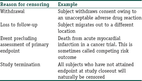
Note that if we visualize the survival experience of an individual as a time-line, then in the examples given in Table 1, the event, assuming it were to occur, would have occurred beyond the end of the follow-up period. This situation has been referred to as right censoring. Death itself is a common cause of right censoring in long-term studies where it is not the outcome of interest. Censoring can also occur if we are interested in an outcome but do not know exactly when it has occurred. For instance, if we are looking out for relapse of a cancer, and following up the patients every 3 months after completion of primary treatment, we will not know exactly when the relapse has occurred for a subject who is diagnosed with a recurrence at 3 months. This is left censoring. It is also possible to encounter interval censoring, meaning that both the entry and exit points are not known precisely. Thus, in the recurrence example, those who are disease free at 3 months, diagnosed with recurrent cancer at 6 months, and lost to follow-up at 9 months are considered interval censored. Most survival analyses deal with right censoring.

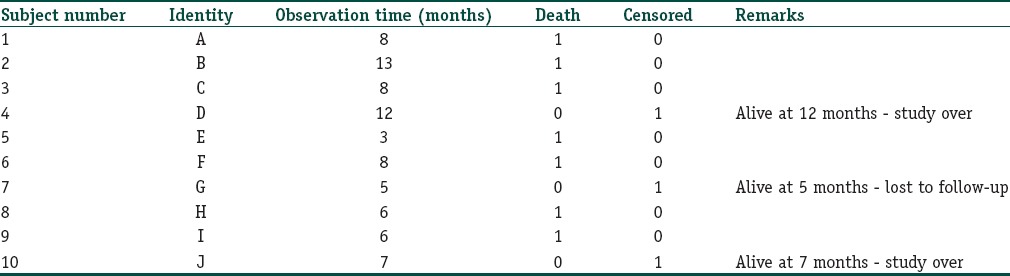
As shown in Figure 1, we have depicted the entry and exit points for 10 subjects in a hypothetical study of malignant melanoma with death events. The survival data from this figure are extracted to a format conducive to survival analysis as shown in Table 2. Note that in the parlance of survival analysis, subjects who experience the event in question may be regarded as “failures” while those who do not are “survivors.”

Figure 1.

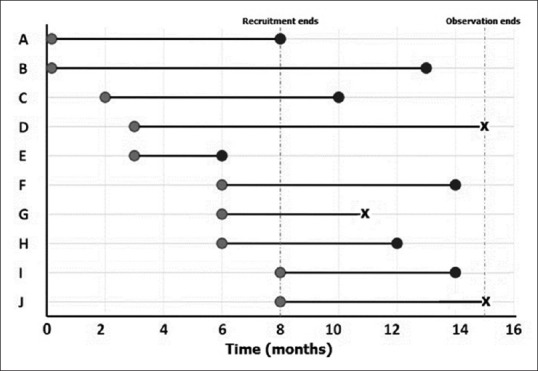
Typical timelines for survival analysis. That recruitment and end of observation for individual subjects occur at varying time points. Event in question is denoted by black circles, while censoring is indicated as X marks

Table 2.

Basic data tabulation for survival analysis

A frequently asked question is that if there are no censored observations in a time-to-an-event study, is survival analysis needed? Not necessarily, we could use usual descriptive measures (such as median and interquartile range) to summarize and nonparametric tests (such as the Mann–Whitney U-test) to compare survival times between groups. However, the survival method lends itself to unique mode of data display and can yield estimate of risk that is often required.

Survivor and Hazard Functions

Survival data are usually described in terms of two related probabilities, namely, survival and hazard. The survival probability, also called the survivor function, S (t), is the probability that an individual survives from a specified time point (e.g. the diagnosis of cancer) to a specified future time t. The multiplication rule of cumulative probability applies in calculation of S (t). If we toss a fair coin, the probability of getting a head is 0.5. If we toss the coin a second time, the probability of getting a head is 0.5. The probability of getting two heads in succession is 0.5 × 0.5, i.e., 0.25. Similarly, the probability of a person surviving for n number of years is the product of the probabilities of survival in year 1, year 2, year 3, and so on till year n, i.e., p1 × p2 × … p (n − 1) × p (n). The survivor function summarizes directly the survival experience of a study cohort and is crucial to analyzing time to event data.

“Hazard” is indicative of the rate at which a particular event occurs. Hazard function is usually denoted as h (t) and represents the probability that an individual who is under observation at time t has an event at that time. In other words, it represents the instantaneous event rate for an individual who has already survived to time t. Note that, in contrast to the survivor function, which relates to not having an event, the hazard function relates to the event occurring. Hazard relates to the incident (current) event rate, while survival reflects the cumulative nonoccurrence. Unfortunately, unlike S (t), there is no simple way to estimate h (t). Instead, a statistic called the cumulative hazard H (t) is commonly used. This is defined as the integral of the hazard, or the area under the hazard function between times 0 and t. The interpretation of H (t) is difficult, but it may be thought of as the cumulative force of mortality, or the number of events that would be expected for each subject by time t if the event were a repeatable process. H (t) is used an intermediary measure for estimating h (t) and as a diagnostic tool in assessing model validity.

Mathematical relationships between S (t) and h (t) have been defined, and computer software makes use of these functions to return the value of one probability if the other is known.

Techniques and Prerequisites in Survival Analysis

Several methods exist for doing survival analysis. Broadly, these can be regarded as parametric, semi-parametric, and nonparametric methods. The difference between the methods lies in the assumptions that we make regarding the distribution of the survival data. However, all survival analysis methods can handle censored data.

Descriptive methods for estimating the distribution of survival times from a sample include life table analysis, Kaplan–Meier analysis, and various types of distribution fitting. Several techniques are available for comparing the survival in two or more groups. Finally, survival analysis offers different regression models for estimating the relationship of predictors to survival times. The most commonly used regression method is the Cox proportional hazards regression, which is a semi-parametric method. We will now take a look at some of these techniques.

An important point to note is that standard methods used to analyze survival data with censored observations, which we are going to discuss, are valid only if the censoring is “noninformative,” that is, carries no prognostic significance about the subsequent survival experience. In other words, subjects who are censored (because of loss to follow-up) should be as likely to suffer the event as those remaining in the study. If subjects keep withdrawing because of worsening clinical condition or adverse drug reactions, the censoring has prognostic implications. Standard methods for survival analysis are not valid when there is informative censoring. Fortunately, when the number censored are small, say < 10%, the resulting bias is likely to be small and can be ignored.

The length and completeness of follow-up are other important prerequisites for reaching valid conclusions from analysis of survival data. Time to event studies must have sufficient follow-up to capture enough events to ensure that there is sufficient power to perform relevant statistical tests. For instance, a 2-year follow-up would be adequate for studying survival in pancreatic cancer, which has poor prognosis, but would be grossly inadequate for breast cancer which has much better prognosis. The median follow-up time is an indicator of the length of follow-up and should be estimated and stated. Although censoring is an accepted phenomenon in survival analysis, the completeness of follow-up is still important so as not to miss events unduly. Unequal follow-up between different treatment groups may produce biased results. In fact, disparities in follow-up caused by large inequalities in dropout rates between treatment arms may carry prognostic implications regarding the treatments.

Cohort effect on survival is another area of concern. Survival analysis generally assumes that there is homogeneity of treatment and other factors during the follow-up period. Thus, subjects recruited relatively early and relatively late in a long-term survival study should not represent separate cohorts with respect to their baseline risk or the nature of the treatment they undergo. If there is possibility of such cohort effects, the assumptions may need to be tested through subgroup analysis and adjustments made accordingly for further analysis.

Kaplan–Meier Technique

The life table or actuarial technique is one of the oldest methods for analyzing survival time data. In this technique, the distribution of survival times is divided into a certain number of time intervals. However, Kaplan and Meier (after Edward Lynn Kaplan and Paul Meier, 1958) showed that rather than classifying the observed survival times into a life table with fixed time intervals, it is possible to estimate the survivor function directly from the actual survival times. The Kaplan–Meier approach uses the exact time of death in the calculation of survival.

In contrast to a conventional life table with fixed time intervals, a Kaplan–Meier life table will have varying intervals and each time interval would contain exactly one case (and any number of observations that got censored since the last interval). Calculation of the survivor function requires multiplying out the survival probabilities across the “intervals” (i.e., for each single event) that are obtained.

Calculation-wise, suppose that k subjects have events in the period of follow-up at distinct times t₁, t₂, t₃,…., t_k. As events are assumed to occur independently of one another, the probabilities of surviving from one interval to the next may be multiplied together to give the cumulative survival probability. More formally, the probability of being alive at time t_j, S (t_j), is calculated from S (t_{j − 1}), the probability of being alive at time t_{j − 1}, n_j the number of subjects alive just before t_j, and d_j the number of events at t_j, as

S (t_j) = S (t_{j − 1}) × (1–d_j/n_j)

Where t₀ = 0 and S₀ = 1.

The value of S (t) is constant between events, and therefore, the estimated probability is a step function that changes value only at the time of each event. If every subject experienced the event, that is, if there is no censoring, this estimator would simply reduce to the ratio of the number of subjects’ event free at time t divided by the number of subjects who entered the study. The method is called product limit estimation because of the nature of this calculation.

The cumulative probability of survival, so calculated, if plotted against time, gives a staircase diagram as shown in Figure 2 which is called a Kaplan–Meier survival plot. It is a crazy staircase though with neither the height nor the width of the “stairs” fixed. The plot takes a dip every time an event occurs. Censored observations may be indicated as points on the steps, corresponding to their last observation time. Confidence intervals for the survival probability can also be calculated. These usually widen over time because the number of subjects decreases. A table indicating numbers at risk may be appended below the time axis to indicate this change in numbers over time.

Figure 2.

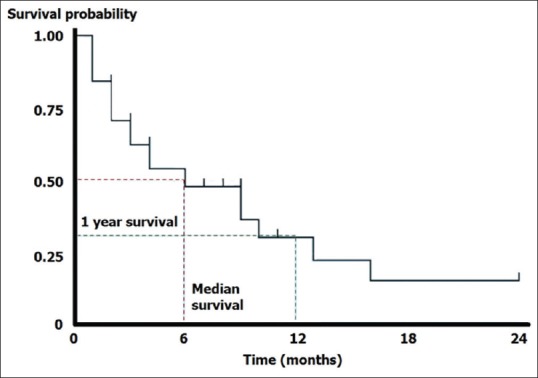
A basic Kaplan–Meier survival plot. That censoring is indicated in this plot by small ticks on the steps

Note that such a plot need not depict only survival data. If the event in question is a “positive” event (like recovery from an acute illness) rather than a “negative” event (like death), the “staircase” would be ascending rather than descending.

The Kaplan–Meier plot provides a useful summary of survival data and can be used to estimate measures such as median survival time, which is simply read off at the 0.5 survival probability. The large skew encountered in the distribution of most survival data implies that the mean is not used and the method itself is regarded as distribution free or nonparametric. Note that we cannot read off survival probabilities which are below the lower limit of the curve. Thus, if the plot does not dip down to the 0.5 survival probability level, we cannot read off the median survival.

Finally, remember some of the pitfalls of the Kaplan–Meier curve

• Curves that have many small steps usually have a higher number of participating subjects, whereas curves with large steps usually have a limited number of subjects and tend to be less accurate

• Most studies have a minimum duration of follow-up based on knowledge of disease biology and overall survival. At this minimum duration of follow-up, the status of each patient is known. The survival rate at this point becomes the most accurate reflection of the survival rate of the group. At the end of the survival curve, there are far fewer patients remaining and thus survival estimates at the end of the curve are less accurate

• When patients are censored, we do not know whether they have actually experienced the outcome of interest. Thus, more the number of patients who are censored, the less reliable is the Kaplan–Meier curve.

Comparing Survival Times between Groups

Survival times in two or more groups or subgroups often need to be compared. In principle, because survival times are not normally distributed, nonparametric tests that are based on the rank ordering of survival times (such as Mann–Whitney U-test or Kruskal–Wallis test) should be applicable. However, conventional nonparametric tests cannot be used to compare survival times since they cannot handle censored observations.

The tests capable of handling censored data include:

• Log-rank test (first proposed by Nathan Mantel), also referred to as Mantel–Haenszel log-rank test (after Nathan Mantel and William Haenszel) or Mantel–Cox test (after Nathan Mantel and David Roxbee Cox)

• Peto and Peto's version of the log-rank test (after Richard and Julian Peto)

• Gehan's generalized Wilcoxon test or Gehan–Breslow–Wilcoxon test (after Edmund Alpheus Gehan, Norman Edward Breslow and Frank Wilcoxon)

• Peto and Peto's generalized Wilcoxon test or Peto–Peto–Prentice test (after Richard and Julian Peto and Ross Prentice)

• Tarone–Ware test (after Robert E. Tarone and James Ware)

• Fleming–Harrington test (after Thomas R. Fleming and David P. Harrington).

These tests can be used to assess statistical significance of differences in time to event between groups. It is important to note that most of these tests will only yield reliable results with fairly large sample sizes. There are no widely accepted guidelines concerning which test to use in a particular situation. The Gehan–Breslow–Wilcoxon method gives more weight to deaths at early time points, which makes sense. However, the results can be misleading when a large fraction of patients are censored early on. In contrast, the log-rank test gives equal weight to all time points and is the more powerful of the two tests if the assumption of proportional hazards is true. Proportional hazards means that the ratio of hazard functions (deaths per time) is the same at all time points. Thus, if deaths in the control group occurred at twice the rate as in the treated group at all time points, the proportional hazards assumption is true. Therefore, the generalized Wilcoxon tests are more likely to detect early differences in the two survival curves whereas the log-rank test is more sensitive to differences at the right tails. If Kaplan–Meier survival curves cross, this indicates nonproportional hazard, in which cases alternatives to the log-rank test such as Peto–Peto Prentice, Tarone–Ware, or Fleming–Harrington tests may need to be used.

More about Log-rank Test

The log-rank test is a nonparametric hypothesis test to compare the survival trend of two or more groups when there are censored observations. It is widely used in clinical trials to compare the effectiveness of interventions when the outcome is time to an event. The test was first proposed by Nathan Mantel and was named the log-rank test by Richard and Julian Peto. It is also known as the Mantel–Cox test and can be regarded as a time-stratified version of the Cochran–Mantel–Haenszel Chi-square test.

The null hypothesis for the test is that that there is no difference in the survival experience of the subjects in the different groups being compared. Its name derives from its relation to a test that uses the logarithms of the ranks of the data. There are certain preconditions for applying the test.

• The test assumes no particular distribution for the survival curve, that is, it is distribution free (nonparametric)

• Subjects who are censored have the same probability of the event as subjects who are fully followed up, that is, the censoring must be noninformative

• The proportional hazards assumption must be met, that is, there is no tendency for one group to have better survival than the other group at earlier time points and then worse survival at later time points. Such a tendency would be reflected in Kaplan–Meier plots that diverge initially and then cross.

The test works by dividing the survival scale into suitable intervals according to the observed survival times. Censored survival times are ignored. Assuming the null hypothesis to be true, for each interval, the expected number of deaths are calculated from the observed number of deaths. The calculations continue till all events are accounted for and these are then added across all-time intervals. The observed numbers are finally compared with the expected numbers, assuming a Chi-square distribution with 1 degree of freedom. The resultant P value is interpreted in the usual way, with P < 0.05 indicating a statistically significant difference in the survival experience between the two groups. The test also generalizes to more than two groups. When two groups are being compared, statistical software will often produce an adjusted odds ratio as an estimate of risk of death – this is called the hazard ratio (HR).

Figure 3 provides a hypothetical example of the log-rank test applied to Kaplan–Meier survival curves comparing survival experience between melanoma and metastatic nonmelanoma skin cancer patients. The plots are clearly divergent, indicating worse prognosis for melanoma and the difference is statistically significant. As stated earlier, variants of the log rank test have evolved more recently, to take care of situations when the curves cross. These include Peto and Peto's test, Peto–Peto–Prentice test, Tarone–Ware test, Fleming–Harrington test, and others.

Figure 3.

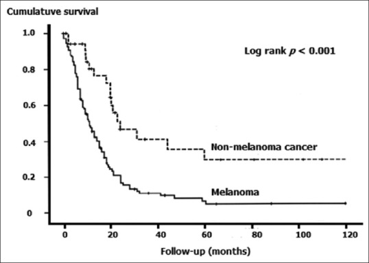
Kaplan–Meier survival plots compared by the log-rank test

Modeling Risk Factors that Influence Survival Time

Advanced survival analysis makes use of modeling techniques to assess if the survival experience conforms to predictive mathematical models and to identify predictor variables that influence survival time. When it is of interest to determine whether or not certain independent predictors influence the survival time, there are two major reasons why this issue cannot be addressed via straightforward linear regression techniques. First, the dependent variable of interest (i.e., survival or failure time) is most likely not normally distributed, which is a serious violation of the assumption for conventional least squares multiple regression. Second, there is the problem of censoring. Therefore, separate regression models need to be used. Examples are the Cox proportional hazard model, exponential regression, and log-normal regression

Cox proportional hazard model (after David Roxbee Cox, 1972) is the most general of the regression methods that allow the hazard function to be modeled on a set of explanatory variables without making restrictive assumptions concerning the nature or shape of the underlying survival distribution. It can accommodate any number of covariates, whether they are discrete or continuous. The model assumes that the underlying hazard rate (rather than survival time) is a function of the independent variables (covariates); no assumptions are made about the nature or shape of the hazard function.

Similar to the adjusted odds ratios in logistic regression, this Cox's proportional hazard technique produces adjusted HRs according to the influence of the modifying factors. HR >1 (with appropriate 95% confidence limits) indicates that the covariate is associated with increased risk, keeping other covariates constant. Common covariates selected when modeling survival include patient's age, gender, and baseline risk status.

While no assumptions are made about the shape of the underlying hazard function, the model does assume a multiplicative relationship between the underlying hazard function and the potential predictors after certain mathematical derivations. This assumption is called the proportionality assumption and gives the model its name. In practical terms, it is assumed that, given two observations with different values for the independent variables, the ratio of the hazard functions for those two observations does not vary with time. However, there are situations where the validity of the proportional assumption is open to question. For instance, when studying survival after stroke, it is likely that age is a more important predictor of early death than later death following initial recovery. The original model has been modified so as to incorporate such time-dependent covariates.

Examples from Published Literature

Survival analysis is not often required in dermatology, apart from the study of skin cancers. However, before we conclude, we would like to provide a few interesting examples [Box 1].

Box 1. Examples of survival analysis from published literature.

Fujii K, Kanno Y, Konishi K, Ohgou N. A specific thrombin inhibitor, argatroban, alleviates herpes zoster-associated pain. J Dermatol 2001;28:200-7.

Fujii et al. conducted an open label, randomized, controlled trial of antithrombin therapy for herpes zoster-associated pain. Fifty-five herpes zoster patients were enrolled in the trial within 8 days after the onset of skin lesions. Patients were treated with an optimal dose of oral aciclovir for 7 days with or without intravenous administration of the specific thrombin inhibitor, argatroban, three times a week. Pain intensity was assessed by the visual analog scale. Administration of argatroban shortened the median time to cessation of analgesic use (14 days vs. 24 days, P=0.02, log-rank test), although it did not significantly reduce the median time to cessation of pain (21 days vs. 43 days, P=0.07, log-rank test). No subject showed adverse effects including hemorrhagic diathesis. The results suggested that relatively low-dose argatroban is effective in reducing herpes zoster-associated pain.

Thompson JM, Li T, Park MK, Qureshi A, Cho E. Estimated serum vitamin D status, vitamin D intake, and risk of incident alopecia areata among US women. Arch Dermatol Res 2016;308:671-6. Studies have identified increased prevalence of Vitamin D deficiency in patients with alopecia areata (AA), but few have prospectively examined Vitamin D status and incident AA. In 55,929 women in the Nurses’ Health Study (NHS), Thompson et al. prospectively evaluated the association between estimated Vitamin D status, derived from a prediction model incorporating lifestyle determinants of serum Vitamin D, and self-reported incident AA. The authors evaluated dietary, supplemental, and total vitamin D intake as additional exposures. Using Cox proportional hazards models, they calculated age-adjusted and multivariate hazard ratios (HR) to evaluate risk of AA. Over a follow-up of 12 years, 133 cases of AA were identified. The age-adjusted HR between top versus bottom quartiles for serum vitamin D score was 0.94 (95% confidence interval [CI] 0.60 to 1.48) and the corresponding multivariate HR was 1.08 (95% CI 0.68 to 1.73). There was no significant association between dietary, supplemental, or total Vitamin D intake and incident AA. Thus, this study did not support a preventive role for Vitamin D against AA.

Dunlap R, Wu S, Wilmer E, Cho E, Li WQ, Lajevardi N, Qureshi A. Pigmentation traits, sun exposure, and risk of incident vitiligo in women. J Invest Dermatol 2017 Feb 14. doi: 10.1016/j.jid. 2017.02.004. [Epub ahead of print]. Although vitiligo is the most common cutaneous depigmentation disorder worldwide, little is known about specific risk factors for its development. Utilizing data from the NHS, Dunlap et al. conducted a prospective cohort study of 51,337 white women to examine associations between pigmentary traits and reactions to sun exposure and risk of incident vitiligo. NHS participants responded to a question about clinician-diagnosed vitiligo and year of diagnosis (2001 or before, 2002–2005, 2006–2009, 2010–2011, or 2012+). They used Cox proportional hazards regression models to estimate the multivariate-adjusted HR and 95% CI of incident vitiligo for the different exposures variables, adjusting for potential confounders. There were 271 cases of incident vitiligo over 835,594 person-years. Vitiligo risk was higher in women who had at least one mole larger than 3 mm in diameter on their arms (HR 1.37, 95% CI 1.02 to 1.83). In addition, vitiligo risk was higher among women with better tanning ability (HR 2.59, 95% CI 1.21 to 5.54) and in women who experienced at least one blistering sunburn (HR 2.17, 95% CI 1.15 to 4.10. Thus, in this study, upper extremity moles, a higher ability to achieve a tan, and history of a blistering sunburn were associated with higher risk of developing vitiligo in white women.

Financial support and sponsorship

Nil.

Conflicts of interest

There are no conflicts of interest.