HUMAN CAPITAL GROWTH AND POVERTY: EVIDENCE FROM ETHIOPIA AND PERU

Abstract

In this paper we use high quality data from two developing countries, Ethiopia and Peru, to estimate the production functions of human capital from age 1 to age 15. We characterize the nature of persistence and dynamic complementarities between two components of human capital: health and cognition. We also explore the implications of different functional form assumptions for the production functions. We find that more able and higher income parents invest more, particularly at younger ages when investments have the greatest impacts. These differences in investments by parental income lead to large gaps in inequality by age 8 that persist through age 15.

1. Introduction

There is an increasing consensus that events and experiences in the early years of childhood, from conception to at least the age of three, have long lasting consequences for an individual’s development and productivity.¹ There is also agreement on the fact that human capital is a multidimensional object, with its various constituents (health, cognition, language, socio-emotional skills) interacting over time along the process of its development, giving rise to complex dynamics and complementarities (see Cunha and Heckman (2008), Cunha, Heckman, and Schennach (2010) and Aizer and Cunha (2012)). These dynamic interactions, together with the possible malleability of skills at certain points in the life cycle, give rise to potential ’windows of opportunity’ for targeted interventions that can improve the development of vulnerable children.²

These issues are particularly relevant in developing countries, where children living in poverty are exposed to a variety of risks, including disease, malnutrition, violence and unstimulating environments. Indeed, the developmental gaps between children living in more versus less affluent families have been amply documented (see Fernald, Weber, Galasso et al. (2011), Carneiro and Heckman (2003), Currie (2008), Rubio-Codina, Attanasio, Meghir et al. (2015), Hart and Risley (1995), and Fernald, Marchman, and Weisleder (2013)).

One way of understanding how these factors interact during childhood to produce life-long outcomes is to estimate production functions for the various dimensions of human capital. These production functions can map the interaction of family background and the current skill level of the individual child, along with investments in the child at each age into child development and growth. This approach is useful because it allows us to identify the degree of persistence of different inputs into development and their influence on subsequent growth. This characterization in turn can be used to identify ’windows of opportunity’: periods in the life cycle of the child where investments (including policy interventions) might be particularly fruitful.

In this paper, we use high quality data from Ethiopia and Peru drawn from the Young Lives Survey to implement this approach, by estimating flexible specifications of the production functions for health and cognition, two key components of human capital. For each of these countries, we have observations for two different cohorts spanning most of childhood. In particular, the younger cohort is observed at ages 1, 5 and 8, while the older cohort is observed at ages 8, 12 and 15. Building on earlier work (see, for example, Cunha and Heckman (2008), Cunha, Heckman, and Schennach (2010), Attanasio, Meghir, and Nix (2015), and Attanasio, Cattan, Fitzsimons et al. (2015)) we follow a factor analytic approach to estimate investment equations and production functions for human capital from age 1 to 15, allowing these to be dynamically connected. Our model can be viewed as an approximation to a dynamic model of household choice and investments in children with liquidity constraints. Del Boca, Flinn, and Wiswall (2014) show how such a dynamic model can be specified and estimated structurally.

Our paper offers innovations in a number of dimensions, including our particular attention on the functional form for the production function and the comparison between two countries. Given the results in Attanasio, Meghir, and Nix (2015), we emphasize the interaction between health and cognition, recognizing that disease and malnutrition can have detrimental effects on cognitive development. We also use their approach to allow for the endogeneity of parental investment decisions, which offers some insight on whether parental investments reinforce or compensate shocks experienced by the children. We experiment with flexible functional forms for the production functions. But perhaps the most important innovation in the paper is the empirical focus on two developing countries, where, with the exception of Attanasio, Meghir, and Nix (2015) in India, child development has not been studied before over such extensive age ranges. Ultimately the hope is that by studying child development in various different low income countries we can identify important regularities that will help us understand the process and design more effective interventions.

We find that the production of health and cognition is quite similar in both Peru and Ethiopia. Specifically, in both countries we find that both cognitive skills and health are very persistent, although health is even more persistent than cognition. We find some evidence that health is cross productive; health positively impacts the production of cognition at early ages. Investments have large impacts on the production of cognition, but the effect decreases with age. We also find in both countries that investments are endogenous and parents compensate for negative shocks. Overall, our results are consistent with a growing body of evidence that early investments in children matter and that the pattern of persistence and dynamic complementarities is a complex one that changes over time as children age (see, for example, Cunha, Heckman, and Schennach (2010), Del Boca, Flinn, and Wiswall (2014), Attanasio, Cattan, Fitzsimons et al. (2015) and Attanasio, Meghir, and Nix (2015)).

Last, we perform a number of counterfactuals. First, we examine the impact of increasing either investments alone or investments and health at age 5 for children with cognitive deficits at age 5. We find that this intervention leads to large gains in cognition which are sustained through age 15. Next, we show that rich and poor children with identical baseline skills will end up with large gaps in cognitive skills by age 15 due to the fact that richer parents invest more in their children.

The rest of the paper is organized as follows. In Section 2, we develop the conceptual framework that is used in the empirical analysis. In particular, we sketch the model of human capital accumulation and discuss how different functional forms can have different implications. In Section 3, we discuss the estimation strategy we use and in Section 4 the data. In Section 5, we present our main empirical results, focusing on the cross-country comparisons and the differences across the Nested CES and the CES. In Section 6 we present counterfactual exercises and Section 7 concludes.

2. The Process of Human Capital Development from Age 1 to 15

We consider human capital development over a sequence of periods in childhood, driven by the available spacing of the data. In each period, we specify how current levels of health and cognition are separately determined as the result of a process that combines five different inputs: the child’s past health $({\theta }_{i,t}^H)$, child’s past cognitive ability $({\theta }_{i,t}^C)$, parental investments (I_i,t), parental health $(P_i^H)$, and parental cognition $(P_i^C)$.

In particular, we write the production of a given component of human capital this period, ${\theta }_{i,t+1}^k$, as the result of a production function f_t which takes as inputs the components discussed above:

$${\theta }_{i,t+1}^k=f_t\left({\theta }_{i,t}^C,{\theta }_{i,t}^H,I_{i,t},P_i^C,P_i^H,X_{i,t},A_t^k,{\epsilon }_{i,t}^k\right),k\in \{C,H\}$$ (2.1)

Notice that in addition to the five inputs listed above, we also include a number of other factors that might affect the accumulation of human capital, in a vector X_i,t. These include the gender of the child, the number of siblings in the family, and the number of older siblings. Gender is included to test whether the process of human capital accumulation is different for boys and girls. Note that gender effects could also capture differential investments by parents, if those investments are not fully captured by I_t. For example, we do not have sufficient information on parental time investments in children, so a difference in human capital production by gender could capture differential time investments. The number of siblings may capture differential returns to scale across large and small families: smaller investments in any given child may be overcome by shared investment in siblings.

In addition to observable variables, we allow the production functions for cognition and health to depend on unobserved shocks $({\epsilon }_{i,t}^k)$ and a term meant to capture ‘total factor productivity’ (TFP). The TFP term $(A_i^k)$ is particularly important when estimating different production functions covering several ages since it can flexibly capture growth over time and with age. We discuss issues related to the interpretation of TFP in more detail in the results section.

We pay particular attention to the marginal effects of parental investments and the child’s past skills at different points in time. The derivatives of child skills are important as they play a large role in determining the persistence of the process that governs human capital accumulation. The combination of the marginal effects of investments and child’s past skills determines the degree to which investment may (or may not) have long run effects. Understanding the persistence as well as the immediate impact of investments is clearly crucial for the design of effective interventions and the identification of what have been called ‘windows of opportunities’.³

Equation (2.1) above is a fairly general representation of the production of child human capital. However, while a fully nonparametric production function is identified under conditions defined in Cunha, Heckman, and Schennach (2010), as well as further conditions on the support of the instruments for investments, the dimensionality of the problem makes this a forbidding task, both computationally and in terms of the amount of data required. Even so, a flexible specification can be important for the economic implications of the results obtained from the estimates. In particular, estimates of the productivity of parental investment and its persistence (or fade-out) can be substantially affected by the functional form assumptions used. In what follows, we strive to combine analytical and empirical tractability with flexibility.

The Functional Form of Children’s Human Capital Production

A specification for the production function that has recently been used in the literature on human capital production is the Constant Elasticity of Substitution (CES) production function (see, for instance, Cunha, Heckman, and Schennach (2010)). The CES allows for some degree of flexibility in the way in which inputs interact. In particular, different inputs can be either complements or substitutes. These interactions have important implications for human capital development among children and optimal policies to foster human capital development. Given the two components of human capital we are considering, cognition (C) and health (H), the CES production function is given by:

$$\begin{array}{l}{\theta }_{i,t+1}^k=[{\gamma }_{1t}^k{P}_i^{C_{{\rho }_{tk}}}+{\gamma }_{2t}^k{P}_i^{H_{{\rho }_{tk}}}+{\gamma }_{3t}^k{I_{i,t}}^{{\rho }_{tk}}+\\ {{\gamma }_{4t}^k{{\theta }_{i,t}^C}^{{\rho }_{tk}}+{\gamma }_{5t}^k{{\theta }_{i,t}^H}^{{\rho }_{tk}}]}^{\frac{1}{{\rho }_{tk}}}{e}^{{\varphi }_{tk}^{\prime }{X}_{i,t}+A_t^k+{\epsilon }_{i,t}^k},k\in \{C,H\}\end{array}$$ (2.2)

where the parameters ${\gamma }_{jt}^k$, j = 1, …5, are constrained to sum up to 1 in each period. The term $A_t^k$ captures TFP. Notice that the parental cognition and health variables are assumed not to change over time. In contrast, the parameters of the production function and all other inputs vary with the age of the child.

The CES nests as special cases a linear production function, which occurs when ρ_k = 1 and implies perfect substitutability among the various inputs. It also nests as a special case the Cobb Douglas, which occurs when ρ_tk = 0 and implies that the elasticity of substitution between different inputs is 1. An important limitation of the CES functional form, however, is that it imposes an elasticity of substitution that is the same among any pair of inputs of the production technology: ρ_k is the unique parameter capturing the degree of substitutability among any pair of inputs.

A feasible and more flexible alternative to the CES is the so-called nested CES. Such a specification allows one to explore whether subsets of inputs are complements or substitutes in the production of cognitive or health skills. Inputs are grouped in different sets and each set is aggregated with a CES function, with the resulting ‘intermediate output’ entering another CES function. In principle one can consider many groups of inputs, even pairs, and hence achieve a different degree of substitutability among all different pairs of inputs.⁴ There is, of course, a degree of arbitrariness in the way in which groups of inputs are formed and nested within the outside CES functional.

In this paper, we explore the possibility that initial conditions for child development (given by lagged cognition and health) are combined by a simple CES which is then nested in another CES. This expresses the production of human capital outcomes as a function of the aggregated lagged child skill levels, parental background and investments. This gives the following equation:

$$\begin{array}{r}{\theta }_{i,t+1}^k=[{\gamma }_{1t}^k{P}_i^{C_{{\rho }_{tk}}}+{\gamma }_{2t}^k{P}_i^{H_{{\rho }_{tk}}}+{\gamma }_{3t}^k{I_{i,t}}^{{\rho }_{tk}}+\\ {\gamma }_{4t}^k({\delta }_{1t}^k{{\theta }_{i,t}^C}^{{\rho }_{\mathit{skills},tk}}+{(1-{\delta }_{1t}^k){{\theta }_{i,t}^H}^{{\rho }_{\mathit{skills},tk}})}^{\frac{{\rho }_{tk}}{{\rho }_{\mathit{skills},tk}}}]{ }^{\frac{1}{{\rho }^{t}k}}{e}^{{\varphi }_{tk}^{\prime }{X}_{i,t}+A_t^k+{\epsilon }_{i,t}^k},k\in \{C,H\}\end{array}$$ (2.3)

This specification allows us to test for the existence of cognitive and health skill complementarity in the production of future skills. Notice that equation (2.3) reduces to equation (2.2) when ρ_skills,tk = ρ_tk. The possibility of having different degrees of substitutability among subsets of inputs is relevant since it will affect the marginal productivity of investment in skills. The nested CES allows for greater flexibility in the set of complementarity patterns between initial cognition and health on the one hand and investments on the other, which may be important in understanding how skills develop with age.

3. Estimation

There are two main challenges to estimating the production functions. First, the factors are not directly observed and this leads to a complex measurement error problem. Second, parental investments may be endogenous.

3.1. Extracting the latent factors from a system of measurements

While PPVT scores, math test scores, and language test scores can all be thought of as measuring underlying cognition and the various health measures (such as height for age) as reflecting the underlying latent health, none are a perfect proxies for latent cognition and health respectively. We can view these measurements as error-ridden indicators of these latent unobserved factors. To extract the latent factors from these measurements and remove the measurement error, we use a dynamic latent factor model as developed for nonlinear models in Cunha, Heckman, and Schennach (2010), building on work from Hu and Schennach (2008) and Schennach (2004). We use their framework to identify our latent factors of interest from the rich set of measurements in our data. As they show, provided we have 2K measurements on a set of K factors in which we are interested, we can use the multiplicity of measurements for each factor to extract the true, unobserved latent factor, despite the presence of measurement error. While extracting the true, latent factor from the set of available proxies is a nontrivial exercise, Cunha, Heckman, and Schennach (2010) show that the alternative - to estimate production functions using a proxy for each factor, ignoring measurement error concerns - performs poorly, even when using the most informative proxy for each factor.

Letting m_j,k,t denote the jth available measurement relating to latent factor k in time t, we assume a semi-log relationship between measurements and factors

$$m_{j,k,t}=a_{j,k,t}+{\lambda }_{j,k,t}ln({\theta }_{k,t})+{\epsilon }_{j,k,t}$$ (3.1)

where λ_j,k,t is a factor loading, a_j,k,t are constants, and ε_j,k,t are zero mean measurement errors, which capture the fact that the measurements are imperfect proxies of the underlying factors. We assume that the measurement error is independent of the latent factors, which is necessary for identification. We also assume that the measurement errors are independent of each other (across both contemporaneous latent factors and time).⁵

To identify the model we must also scale and normalize the measurements (Anderson and Rubin (1956)). We use the same normalizations used in Cunha, Heckman, and Schennach (2010), setting the first factor loading for each measurement to 1 and normalizing the mean of the latent factors to be 0, while including a TFP term. An alternative approach, presented in Agostinelli and Wiswall (2016), normalizes the means and loadings of only the initial factors. Cattan and Nix (in progress) explore alternative methods and estimators and provide Monte Carlo evidence that shows that the approach we are following performs well in samples of the size we are considering.

The interpretation of the estimates of the production function depends on the units of measurement of the latent factors. In some cases, the available measurements are test scores which are ordinal in nature. Ordinal variables introduce some arbitrariness to results, given that any monotonic transformation of a test score conveys the same information. A way round this issue is to anchor all latent factors to a measure with meaningful units such as earnings, as elaborated by Cunha, Heckman, and Schennach (2010). Anchoring will define not only the scaling but the entire monotonic transformation from the latent factor to the measure. ⁶ Here we lack a measure that would make a suitable anchor because we do not possess longitudinal data that will link early test scores to adult outcomes such as earnings. We thus assume that the factor and the measure are related by a semi-log transformation (and the measurement error).

3.2. Determinants of parental investment

In our model, parental investments in children are determined by parental resources (current and over the lifecycle), parents’ expectations regarding the returns to investments in their children, and the prices of investment goods. More specifically, parents select investments taking into account the child’s current level of cognition and health, because the child’s current level of human capital may determine the returns to investments (in particular if there is complementarity between child skills and investments). Additionally, the level of investments may be determined in part by the parent’s own level of cognition and health, both because this may reflect knowledge about the value of investments and because parental characteristics may capture lifetime resources. Gender may also play a role because of gender preferences or even because of perceived differences in the returns to gender in the labor market. Finally, birth order and the number of siblings impact the available material and time resources that parents are able to devote to a given child. This characterization of parental investments can be derived from a problem where parents choose investments to maximize a welfare function whose arguments are child human capital and own consumption, subject to a budget constraint and the technology constraint imposed by the production function of human capital. Estimating the investment equation can provide some insight as to how parents choose to invest in children and ultimately will help us understand some key sources of inequality in this paper.

We assume that parental investments are at least partly motivated by a desire to affect long term outcomes through the formation of human capital, where human capital in this paper consists of health and cognition. This is why the production functions depend on investment. However, in order for the estimates of the production function to be unbiased, we have to assume that all determinants of both investments and human capital formation are fully captured by the remaining inputs into the production function for human capital: parental cognition and health, past child health and cognition, and household composition.

Yet there is an important possible source of endogeneity: the unobserved shocks to the child’s human capital that parents might react to when choosing their investments. For example, parents may decide to compensate for a negative shock, such as an unexpected episode of ill-health or particularly bad quality of education, by increasing their investments in the child. Alternatively, such a shock may be perceived as lowering the returns to investment, in which case investments may also fall.

To address this potential endogeneity of investments, we follow the control function approach used in Attanasio, Meghir, and Nix (2015).⁷ As in that paper, we use household income and regional variation in prices as instruments. These instruments are valid provided differences in prices and income affect future cognition (or health) only through their impacts on investments. The use of prices as instruments requires the assumption that regional variation reflects cost differences rather than differences in demand. Given the longer term determinants of income (such as parental cognition and health) we assume that current income reflects a liquidity shock and not inputs that should also be included in the production function. As a robustness check we also present results where we only use prices as excluded instruments in the appendix. In those specifications, income is included in the production functions in X_i,t as well as in the investment equations.

We approximate the parental investment function using a log-linear specification which takes the form:

$$ln{I}_{i,t}=d_0+d_{1}ln{\theta }_{i,t}^C+d_{2}ln{\theta }_{i,t}^H+d_3{P}_i^C+d_{4}ln{P}_i^H+d_5^{\prime }{X}_{i,t}+d_6^{\prime }\mathit{ln}{q}_{k,t}+d_{7}ln{\gamma }_{i,t}+v_{i,t}$$ (3.2)

where ν_I,t is the error term, X_i,t includes child gender, birth order, and number of children, Y is income, and q_k,t are a set of prices in village k at time t. We can then augment the productions functions to include the residual of the investment function, v_i,t, as a control function. Our estimating equation for the production functions for child health and cognition are then:

$$ln{\theta }_{i,t+1}^k=ln\left(g\left({\theta }_{i,t}^C,{\theta }_{i,t}^H,I_{i,t},P_i^C,P_i^H\right)\right)+{\varphi }_t^k{X}_{it}+A_t^k+{\xi }^k{v}_{i,t}+{\epsilon }_{i,t}^{\ast k}k\in \{C,H\}$$ (3.3)

where the function g(·) is the CES or the nested CES production function outlined earlier and C, H denote cognition and health respectively.

An alternative approach is to solve explicitly for the maximization problem faced by parents and compute the investment function that would result from such a problem, as in Del Boca, Flinn, and Wiswall (2014). Such a function could then be estimated jointly with the production function. Such an approach might be more efficient in certain contexts but does require stronger assumptions about behavior. For example, we do not necessarily require that parents have full knowledge of the parameters of the production function.

3.3. A Three-Step Estimator

As discussed above, the identification of the nonlinear factor model we use is provided in Cunha, Heckman, and Schennach (2010) and is based on the idea of dealing with measurement error in a nonlinear context by using multiple measures for each underlying variable, as in Schennach (2004). The estimation approach we use is described in Attanasio, Meghir, and Nix (2015) and consists of three steps. In the first step, we estimate the joint distribution of the measurements. In addition to the measurements for the latent factors that enter the production function, we also include the variables used as controls (gender, number of children, and so on) and the variables used as instruments for investments (prices and income). Even though no measurement error is considered for these variables, we must include them in this first step in order to recover their relationships with the latent variables. In the second step, we use the measurement system to recover the joint distribution of the latent factors, as well as estimates of the factor loadings and measurement error distribution. With the joint distribution of the latent factors and all other relevant variables in hand, we then generate a synthetic data set by drawing observations from the joint distribution of the factors (including the instruments and controls) and estimate the investment functions and production functions in the third and final step, using nonlinear least squares. Experimenting with the functional form of the production function only involves repeating the relatively simple third step, since the joint distribution of the latent factors completely characterizes all the information in the actual data. For more details on this estimation procedure and its performance, see Attanasio, Meghir, and Nix (2015).

We assume the measurement errors are normally distributed and we approximate the joint distribution of the measurements as a mixture of two normals. These assumptions then imply that the joint distribution of the latent factors is a mixture of normals. The departure from normality is important: the normal distribution has a linear conditional mean. Here the conditional mean is the production function, which means that assuming normality of the latent factors would only allow us to estimate production functions where the inputs are perfect substitutes. More generally, the joint distribution of latent factors must be flexible enough to capture the dependencies in the data and general enough to be consistent with the production function one wishes to estimate. By using an increasingly large number of elements in the mixture the joint distribution can be approximated to an arbitrary degree of precision. Cattan and Nix (in progress) show that a mixture of two normals is sufficient to capture a CES production function.

4. Data

To estimate the production functions, we use data selected from the Young Lives Survey. This is a longitudinal survey covering 12,000 children in four countries: Ethiopia, India, Peru, and Vietnam.⁸ The survey began in 2002 with two cohorts of children in each of these countries. In 2002, the younger cohort was between 6 and 18 months and the older cohort was between 7.5 and 8.5 years of age. The second wave of the survey took place in 2006–2007, and the third wave took place in 2009.⁹

In Ethiopia, the sample selected children from five regions out of nine in the country: Addis Ababa, Amhara, Oromiya, SNNP (Southern Nations, Nationalities and People’s region) and Tigray. These five regions account for 96% of Ethiopia’s total population. Within each region, three to five districts were selected to obtain a balanced representation of poor rural and urban households, as well as relatively less poor rural and urban households. In total, 20 districts are included in the sample. Within the districts, at least one peasant association (in rural areas) or one kebele (i.e. the lowest level of administration for urban areas) was selected and was included as sites if they contained a sufficient number of households with children in the relevant age range. Note that sites were chosen to oversample areas where food deficiency is particularly relevant, as well as to capture Ethiopia’s diversity in terms of ethnicities, in both rural and urban areas. The households participating in the survey were randomly selected within sites.¹⁰

In contrast to the other countries in Young Lives, Peru chose the 20 sentinel sites using a multi-stage, cluster-stratified random sampling approach. However, as in Ethiopia, the 20 sites considered for the multi-stage, cluster-stratified random sampling were chosen so as to over-represent poorer districts (this was achieved by excluding the richest 5% of districts from the sample according to the poverty map developed in 2000 by the Fondo Nacional de Cooperacion para el Desarrollo). The poverty ranking of districts is constructed taking into account factors such as infant mortality, housing, schooling, infrastructure, and access to services. The sample covers households from the following regions of Peru: Tumbes, Piura, Amazonas, San Martin, Cajamarca, La Libertad, Ancash, Huanuco, Lima, Junin, Ayacucho, Arequipa and Puno.¹¹

The surveys are extremely detailed, and we use information from household questionnaires, child questionnaires, and community questionnaires. In Table 1, we present statistics on the children and their households. In Ethiopia, the younger cohort includes 1,999 children and the older cohort includes 1,000 children. By age 5, the average number of children in the household is approximately 4. In the older cohort, by age 12 the same figure is around 6. On average, the focus child in the younger cohort has 2 older siblings at age 5 while children in the older cohort have 3 older siblings at age 12. These relatively high numbers reveal demographic characteristics that are typical of developing countries, which often display households with a relatively high number of children.

Table 1.

Summary Statistics: Demographic Variables

	Younger Cohort			Older Cohort
	Age 1	Age 5	Age 8	Age 8	Age 12	Age 15
Ethiopia
Demographics
Number of Children	3.18 (2.02)	4.14 (2.31)	. .	4.62 (2.14)	5.61 (2.47)	. .
Number Older Siblings	. .	2.44 (2.25)	. .	. .	2.84 (2.45)	. .
Measures of Economic Well Being
Annual Income	. .	5,742 (17,619)	12,800 (35,846)	. .	5,680 (11,097)	12,585 (22,452)
Wealth Index	0.21 (0.17)	0.28 (0.18)	0.33 (0.18)	0.22 (0.17)	0.30 (0.17)	0.35 (0.17)
Number of Observations		1999			1000
Peru
Demographics
Number of Children	2.51 (1.85)	3.15 (2.05)	. .	3.5 (1.9)	4.0 (2.14)	. .
Number Older Siblings	. .	1.61 (1.95)	. .	. .	1.9 (2.13)	. .
Measures of Economic Well Being
Annual Income	. .	12,394 (15,737)	11,691 (19,782)	. .	12,843 (11,980)	11,943 (18,425)
Wealth Index	0.42 (0.19)	0.47 (0.23)	0.54 (0.21)	0.46 (0.19)	0.52 (0.23)	0.59 (0.19)
Number of Observations		2052			714

Consistent with the aims of the Young Lives sampling approach, the households in our sample are relatively poor. This is captured in the summary statistics on average annual income and the wealth index. Average annual income in Ethiopia is computed taking into account income from both wages and benefits. The wealth index is computed by Young Lives as an average of three indices that measure housing quality, consumer durables, and access to services. Average annual income in round 2 is around 6,000 Ethiopian Birr, and around 13,000 Ethiopian Birr in round 3. The high standard deviation of the wealth index reveals the degree of heterogeneity in terms of economic background in the Ethiopian sample, but could also be indicative of measurement error. Given this fact, we will use both the wealth index and measured income as measurements on latent income.

The younger cohort in Peru includes 2,052 children, whereas the older cohort includes 714 children. Peru is a relatively more developed country, and this is reflected in the summary statistics in Table 1. In particular, the average number of children in the household is 3 by age 5, and 4 by age 12. Also, the average number of older siblings is approximately 2 for both samples. In terms of economic well-being, average annual income is approximately 12,000 Peruvian Sols in rounds 2 and 3. The Young Lives wealth index displays relatively less variance with respect to Ethiopia.

In Tables 12–13 in the Appendix we report the summary statistics for the child measurements associated with each latent factor at each age. These measurements demonstrate the richness of data available in the Young Lives data set, which we take full advantage of in our approach. For example, the survey administered a number of tests, including the PPVT, a math test, the CDA test, and the Early Grade Reading Assessment (EGRA), which we use to identify latent cognition for ages 5, 8, 12, and 15. For age 1, no measurements for cognition are available, reflecting the fact that it is almost impossible to measure cognition when children are under the age of 1. In addition, the survey measured weight, height, and elicited self-reported (by either the parent or child) health status, which we use to identify latent health for ages 1, 5, 8, 12, and 15. Assignment of measurements to the remaining factors (investments and parental health and cognition) are discussed in Section 5.1.

5. Results

We organize our results as follows. We first present and discuss the estimates of the measurement system. These estimates identify the joint distribution of the latent factors (child health and cognition, parental investments, and parental health and cognition) and the other variables that make up the production functions. Next, we discuss the determinants of parental investments. Last, we present the results for the production functions. For each set of results, we compare the estimates obtained with the Peruvian and Ethiopian data.

5.1. The measurement system across countries

As described in Section 3.3, the estimation of the measurement system is done in two steps. The estimates of the measurement system are then used to generate synthetic data in the third step. The same synthetic data can be used to estimate both the CES and the Nested CES production functions, given that the same measurement system underlies both production functions.

The estimates of the measurement system can be used to summarize how informative each measurement is in terms of the underlying factor it proxies. In particular, for each measurement used to extract the latent factors, we can compute the signal to noise ratio which is equal to the ratio of the variance of the latent factor to the variance of the measurement error.

In Table 2, we report signal to noise for the measurements we use to identify latent children’s cognitive ability at each age. Also reported in Table 2 are the signal to noise ratios for the measurements we use to identify latent parent’s cognitive ability for the children from each cohort, which is treated as fixed across the different ages. We find that the measurements we use for cognitive skills are very informative, with only a few exceptions (specifically numeracy and writing level are not very informative measurements, which may be related to the limited variability in these measurements).¹² Finally, this and subsequent tables report the factor loading on the log of the factor.¹³

Table 2.

Signal to Noise Ratios for Cognition Measures

Factor	Measures	Ethiopia		Peru
		% Signal	Loading	% Signal	Loading
Child’s Cognitive Skills (Age 5)	PPVT Test	43%	1	86%	1
	CDA Test	25%	0.72	28%	0.63
Child’s Cognitive Skills (Age 8, Younger Cohort)	PPVT Test	36%	1	73%	1
	Math Test	53%	1.23	42%	0.79
	Egra Test	28%	0.94	36%	0.74
Child’s Cognitive Skills (Age 8, Older Cohort)	Ravens Test	–	–	20%	1
	Reading Level	59%	1	62%	1.69
	Writing Level	52%	0.94	44%	1.46
	Numeracy	12%	0.48	5%	0.48
Child’s Cognitive Skills (Age 12)	PPVT Test	36%	1.13	59%	1
	Math Test	24%	1	42%	0.86
	Reading Level	15%	0.76	23%	0.63
	Writing Level	–	–	2%	−0.19
Child’s Cognitive Skills (Age 15)	PPVT Test	43%	1.02	54%	1
	Math Test	36%	1	38%	0.86
	Cloze Test	39%	1.04	58%	1.03
Parental Cognitive Skill (Younger Cohort)	Mom Education	79%	1	62%	1
	Dad Education	33%	0.65	40%	0.82
	Literacy	43%	0.78	46%	0.87
Parental Cognitive Skill (Older Cohort)	Mom Education	8%	1	27%	1
	Dad Education	28%	0.70	40%	0.93
	Literacy	74%	0.79	64%	0.81

In Table 3, we report signal to noise for the measurements used to proxy child health across all ages. We find that with the exception of self-reported health status¹⁴, the measurements on child health are extremely informative regarding latent health: their signal to noise ratios all exceed 50%. The parental health measurements are marginally less informative. Finally, in Table 4, we report signal to noise ratios for the measurements used to proxy investments in children across all ages. The results in the table show that the majority of our information regarding latent investments is related to expenditures on children. The amounts spent on clothing, shoes, and books are particularly informative.

Table 3.

Signal to Noise Ratios for Health Measures

Factor	Measures	Ethiopia		Peru
		% Signal	Loading	% Signal	Loading
Child’s Health (Age 1)	Height Z-Score	58%	1	60%	1
	Weight Z-Score	77%	1.11	60%	1.00
	Healthy? (0–2)	3%	−0.20	3%	0.24
Child’s Health (Age 5)	Height Z-Score	57%	1	62%	1
	Weight Z-Score	68%	1.09	72%	1.13
	Healthy? (0–2)	1%	−0.09	3%	0.23
Child’s Health (Age 8, Younger Cohort)	Height Z-Score	65%	1	73%	1
	Weight Z-Score	77%	1.09	72%	1.01
	Healthy? (1–5)	2%	0.17	2%	0.17
Child’s Health (Age 8, Older Cohort)	Height Z-Score	45%	1	55%	1
	Weight Z-Score	55%	1.19	66%	1.14
	Healthy? (0–2)	1%	−0.18	1%	0.12
Child’s Health (Age 12)	Height Z-Score	72%	1	60%	1
	Weight	72%	1.01	70%	1.11
	Healthy? (0–2)	1%	−0.13	2%	0.17
Child’s Health (Age 15)	Height Z-Score	69%	1	56%	1
	Weight	81%	1.06	56%	1.04
	Healthy? (1–5)	0%	0.08 15	0%	0.09
Parental Health (Younger Cohort)	Mom Weight	92%	1	34%	1
	Mom Height	5%	0.22	45%	1.11
Parental Health (Older Cohort)	Mom Weight	32%	1	33%	1
	Mom Height	71%	0.30	66%	1.05

Table 4.

Signal to Noise Ratios for Investment Measures

Factor	Measures	Ethiopia		Peru
		% Signal	Loading	% Signal	Loading
Investment (Age 5)	Amount Spent on Books	18%	1	5%	0.33
	Amount Spent on Clothing	31%	0.70	60%	1
	Amount Spent on Shoes	42%	1.03	52%	0.95
	Amount Spent on Uniform	1%	0.41	18%	0.54
	Meals in Day	2%	0.22	1%	0.14
	Food Groups in Day	9%	0.47	3%	0.21
Investment (Age 8)	Amount Spent on Books	17%	1.61	38%	0.88
	Amount Spent on Clothing	4%	1	28%	1
	Amount Spent on Shoes	58%	1.72	51%	1.16
	Amount Spent on Uniform	14%	0.75	10%	0.56
	Meals in Day	4%	0.45	2%	0.23
	Food Groups in Day	6%	0.55	1%	0.13
Investment (Age 12)	Amount Spent on Fees	–	–	6%	1
	Amount Spent on Books	11%	1	41%	2.50
	Amount Spent on Clothing	30%	1.62	55%	2.80
	Amount Spent on Shoes	49%	2.06	38%	2.28
	Amount Spent on Uniform	–	–	5%	0.94
	Meals in Day	13%	1.03	1%	0.43
	Food Groups in Day	20%	1.24	3%	0.69
Investment (Age 15)	Amount Spent on Fees	–	–	6%	1
	Amount Spent on Books	20%	1	33%	2.16
	Amount Spent on Clothing	19%	1.01	46%	2.51
	Amount Spent on Shoes	6%	0.63	43%	2.41
	Amount Spent on Uniform	–	–	9%	1.17
	Meals in Day	4%	0.48	1%	0.31
	Food Groups in Day	6%	0.52	1%	0.34

One drawback of our data is that we do not have sufficient information to split latent investments into separate factors, representing different types of investment. With rich enough data, one could consider different types of investment, such as investment in time and material (as done in Attanasio, Cattan, Fitzsimons et al. (2015)) and separately identify investments in health and cognition.

5.1.1. Cross Country Comparison

The signal to noise ratio for the same measurement is often very different across the two countries. For example, the PPVT test appears to be much more informative in Peru relative to Ethiopia. Similarly, the number of food groups is more informative in Ethiopia than in Peru. In other cases, there are large differences but without a discernible pattern across countries when considering all ages. This is a very interesting result and of relevance for international comparisons and, more generally, for the construction of measures that can be used for such comparisons. There are a number of possible explanations for the differences we observe.¹⁶

It may well be possible that the differences are down to data collection: if the enumerators have different skills collecting data in the two countries this could give rise to very different measurement error structures. The difference in signal to noise ratios across contexts could also arise if there is less variability in a given factor in one country versus the other, but the same amount of noise. This may have to do with how heterogeneous the population is in each of the two surveys. A third hypothesis is that some measurements are not comparable across countries because they have not been adapted in the same way (this explanation is particularly relevant for the cognitive tests but arguably less relevant for measurements like height and weight, which can be uniformly applied across countries). This is a general point and cautions about the use of tests to compare across different contexts. It is likely that all three of these explanations are at work in our context. Provided the differences across contexts are not so severe that they invalidate our assumptions on the measurement system, the approach taken here deals with variability in measurement error across countries by removing it and extracting comparable latent factors, albeit with a scale set by the choice of normalization of the loading.

5.2. The determinants of parental investments in children across countries

As discussed in Section 3.2, parental investment decisions are approximated by a log-linear function. Investments in period t depend on the child’s existing stock of human capital, parental cognition and health, birth order, the number of children in the household, child gender, parental income, and prices of investment goods. Birth order, number of siblings, and child gender could be potential determinants of investment both through the budget constraint and by capturing features of parental preferences. Income is clearly an important determinant of investment as it contributes to the relative tightness of the budget constraint that the household faces. Prices of various goods (at the district level each period) that are related to child development may affect investments through the budget constraint. Specifically, we include a price index for food, a price index for clothing, the price of a notebook (related to costs of education), and the prices of the medicines Mebendazol and Amoxicillin.¹⁷ As noted in our description of the data, child cognition in the first wave of the youngest cohort, when the children were 1, was not measured. For this reason the investment equation for age 5 does not include child cognition.

The investment equations are of interest since they reveal potential links through which child’s and parental characteristics, as well as other covariates, influence parental investment behavior. In addition, the saliency of prices and income are particularly important since we use them as instruments for investments in the production functions. For this reason, in the tables below we report the results of a joint F-test for income and the price variables. As we will also investigate the possibility of not using income as an instrument for investments when estimating the production functions, since income may itself be endogenous, we also report the F-test for the joint significance of the price variables alone.

5.2.1. Ethiopia

The determinants of parental investment in health and cognition in Ethiopia are reported in Table 5, along with 95% bootstrap confidence intervals. We find that parental cognition increases investments at all ages but 15 and parental health affects investment at age 5 and 8, but not at older ages of the child.¹⁸ Perhaps surprisingly, child health and cognition do not affect investments. Birth order and the number of children are also mostly insignificant. However it is remarkable that for children at age 5 investments in males are higher by 16%. Although the male preference is no longer evident at older ages, given the potential importance of investment at early ages this is possibly an important source of gender differences in child development. Consistent with theory, families with higher income invest more. The elasticity is highest at the lowest age and decreases thereafter to just under 0.4. While we cannot establish causality beyond reasonable doubt it is worth remembering that the estimated income effect is conditional on parental background and household composition.

Table 5.

The Coefficients of the Investment Equations - Ethiopia

	Age 5	Age 8	Age 12	Age 15
Cognition		0.013 [−0.03,0.08]	0.014 [−0.02,0.07]	0.154 [−0.03,0.31]
Health	0.022 [−0.03,0.06]	0.004 [−0.03,0.04]	−0.001 [−0.03,0.07]	0.027 [−0.04,0.07]
Parental Cognition	0.133 [0.07,0.22]	0.196 [0.12,0.23]	0.04 [0.01,0.12]	0.094 [−0.02,0.18]
Parental Health	0.066 [0.02,0.12]	0.052 [0.02,0.1]	0.012 [0,0.05]	0.008 [−0.02,0.07]
Price Clothes	0.164 [0.02,0.29]	0.132 [0.06,0.18]	−0.063 [−0.27,0.12]	0.081 [−0.05,0.17]
Price Notebook	0.045 [−0.35,0.44]	−0.193 [−0.29,−0.05]	0.037 [−0.17,0.44]	0.133 [−0.09,0.34]
Price Mebendazol	−0.007 [−0.04,0.03]	−0.055 [−0.16,0.03]	−0.044 [−0.09,0.01]	−0.358 [−0.47,−0.2]
Price Amoxicillin	0.038 [−0.03,0.09]	−0.208 [−0.28,−0.16]	0.049 [−0.05,0.14]	−0.056 [−0.19,0.06]
Price Food	0.01 [−0.03,0.07]	−0.044 [−0.09,0.01]	0.013 [−0.09,0.09]	−0.024 [ −0.1,0.02]
Older Siblings	0.053 [−0.02,0.1]	0.033 [−0.02,0.08]	−0.032 [−0.07,0.01]	0.033 [−0.02,0.07]
Number of Children	−0.076 [−0.12,0]	0.005 [−0.04,0.07]	0.054 [0.01,0.09]	−0.006 [−0.04,0.02]
Gender	0.16 [0.07,0.23]	−0.059 [ −0.14,0.03]	0.06 [−0.04,0.17]	−0.033 [−0.14,0.07]
Income	0.644 [0.46,0.83]	0.284 [0.11,0.45]	0.371 [0.14,0.48]	0.367 [0.12,0.47]
Prices and Income (P-values)	0	0	.0010	.0003
Prices (P-values)	.2671	0	.5772	.0003

Notes: 95% confidence intervals based on 100 bootstrap replications in square brackets.

Turning to the joint significance of the variables we use as instruments in the production function, we find that when we consider income and prices jointly, the p-values for the null of no joint significance are very low. However, when we consider only the price variables, we find that they are only jointly significant at ages 8 and 15. In these cases what stands out is the price of the notebook (age 8) reflecting educational costs at that critical age, the price of the deworming drug Mebendazol at age 15, and the price of the antibiotic Amoxicillin at age 8. These estimates imply that a 10% increase in the price of a notebook at age 8 would lead to a 1.93% decrease in investments, a 10% increase in the price of Mebendazol at age 15 would lead to a 3.58% reduction in investments, and a 10% increase in the price of Amoxicilin would lead to a 2.08% decrease in investments at age 8.

5.2.2. Peru

The estimated coefficients of the investment equations for Peru are reported in Table 6. Here again neither child cognitive skills nor child health are significant determinants of investment at any age. This result is potentially important because, as we will see next, investments and child cognition are complementary which implies that the returns are higher for children with higher initial levels of cognition. Perhaps parents are not aware either of the level of cognition of their child or of the parameters of the production functions for human capital.¹⁹ The exception is that child health has a positive effect on investments at age 8.

Table 6.

The Coefficients of the Investment Equations - Peru

	Age 5	Age 8	Age 12	Age 15
Cognition	−	−0.011 [−0.09,0.03]	0.088 [−0.06,0.17]	−0.021 [−0.08,0.04]
Health	0.007 [−0.1,0.03]	0.082 [0.01,0.13]	−0.051 [−0.09,0.02]	−0.024 [−0.08,0.05]
Parental Cognition	0.094 [−0.02,0.18]	0.088 [−0.01,0.15]	−0.048 [−0.14,0.11]	0.018 [−0.09,0.17]
Parental Health	0.072 [0,0.24]	−0.002 [−0.12,0.11]	0.067 [−0.03,0.12]	0.002 [−0.09,0.08]
Price Clothes	−0.003 [−0.16,0.12]	0.099 [−0.01,0.21]	0.304 [0.14,0.43]	0.163 [−0.01,0.29]
Price Notebook	0.217 [−0.05,0.51]	−0.315 [−0.48,0.03]	−0.84 [−1.73,−0.36]	−0.356 [−0.89,0.34]
Price Mebendazol	−0.069 [−0.18,−0.02]	−0.05 [−0.12,−0.01]	−0.075 [−0.2,0.06]	−0.153 [−0.25,−0.05]
Price Amoxicillin	0.053 [−0.01,0.17]	0.058 [−0.03,0.12]	−0.01 [−0.18,0.14]	−0.037 [−0.23,0.08]
Price Food	0.567 [0,1.07]	1.103 [0.73,1.5]	−0.621 [−1.4,0.63]	0.251 [−0.32,0.77]
Older Siblings	0.012 [−0.05,0.06]	0.02 [−0.06,0.05]	0.052 [0,0.09]	0.055 [0.01,0.1]
Number of Children	−0.087 [−0.13,−0.03]	−0.058 [−0.09,0.01]	−0.104 [−0.15,−0.05]	−0.081 [−0.12,−0.04]
Gender	0.009 [−0.08,0.08]	−0.042 [−0.1,0.04]	−0.127 [−0.24,0.03]	−0.183 [−0.29,−0.05]
Income	0.611 [0.48,0.79]	0.567 [0.47,0.85]	0.132 [0.01,0.37]	0.219 [0.07,0.39]
Prices and Income (P-values)	.0001	0	.0113	.0498
Prices (P-values)	.1753	0	.0112	.0354

Notes: 95% confidence intervals based on 100 bootstrap replications in square brackets.

As in Ethiopia, parental cognition seems to matter early on at ages 5 and 8, although the effects are not as strong in Peru. Nevertheless, the result we obtain with the Ethiopian data also holds in the Peruvian context: at older ages child investments do not depend on parental cognition. Parental health matters when the child is 5 but not later. The number of children reduces investments at all ages (although it is not significant at age 8). In contrast, investments are higher for children with older siblings at later ages, perhaps because older siblings are independent earners and more resources are available (conditional on the overall lower investments in families with many children). In Peru, we find no evidence of male preference in investments. Finally, income plays a critical role in investments with the impact being highest for younger children, as in Ethiopia. In Peru, we see a much more pronounced decline of the income effect as the child ages. However, what stands out is that in both cases income matters most at the youngest age suggesting that poorer parents invest substantially less at an age where these investments may be critical for child development. We will explore the broader implications of this fact, combined with what we find regarding the production function parameters over these ages, at the end of the paper.

Jointly prices are significant at all ages but the youngest. However, the price of clothing and the price of food enter with the ‘wrong sign’. As discussed above, the likely reason for this result is the source of (regional) variation in prices that we are exploiting. What stands out as before is the price of the notebook at all ages except the youngest (although it is only significant at the 5% level at age 12), and the price of Mebendazol at all ages (although at age 12 it is not significant).

5.2.3. Summary

The one unambiguous result across both countries is that investment in children is driven by income conditional on both parental background and child health and cognition. We interpret this as the impact of current resources. Importantly, the effect of income is highest for the youngest children, meaning that differences in investments across income groups are highest at the youngest ages. This holds true in both countries. The quality/quantity trade-off is only apparent in Peru and male preference is evident at younger ages in Ethiopia.

Finally, there is evidence that prices matter, particularly those relating to health care and education. We rely exclusively on spatial variation, which we assume is not driven by to demand differences. However, this is clearly not the ideal data set to identify robust price effects. Some of the perverse price impacts may well be due to a violation of the price exogeneity (due to shifts in preference for child goods across regions). Notice that violation of price exogeneity does not jeopardize our ability to identify the parameters of the production function, as long as the ‘shocks’ to prices or the demand shifts across regions that are the cause of endogeneity are orthogonal to the shocks to the human capital production function that cause the endogeneity of investment.

5.3. Production function estimates across countries

Investments reflects parental choices. The next step is to estimate the way these choices, together with the child’s background, affect the production of cognition and health over the various stages of the child’s life. We explore different functional forms for the production functions of child human capital. We first report estimates of CES production functions, which until now has been the most flexible functional form estimated in this literature. We then move on to consider a less restrictive specification, given by the nested CES. Specifically, we estimate the parameters of equations 2.2 and 2.3 with one adjustment at age 5. As in the case of investment, the production functions estimated for age 5 do not include cognitive skills in the previous period as an input, since we have no measures on cognition at age 1.

5.3.1. Constant Elasticity of Substitution (CES) Production Functions: Results and Cross Country Comparisons

In Tables 7 and 8, we present the results from estimating CES production functions for each country. In both tables, investment is considered as endogenous and the coefficients are obtained with a control function approach, using prices and income as excluded instruments, as described above. The assumption underlying the exclusion of income is that conditional on parental and child background as well as the various demographics, income represents a liquidity shock and does not reflect omitted skills and characteristics of the parents that directly affect the production of child human capital. In the appendix we experiment with using just prices as exclusion restrictions. However, as discussed above, prices are not necessarily exogenous either: we still need to assume that either the demand functions for investment are the same across regions over which we have spatial price variation, or at least that any shocks to demand across regions are orthogonal to shocks to the production of human capital that are correlated with parental investments. In general finding the right instruments is an important but hard task and one hopes that in future we can exploit randomized or quasi-experimental variation.

Table 7.

Production of Human Capital, CES Production Function, Ethiopia

	Cognition				Health
Age	5	8	12	15	5	8	12	15
Cognition		0.354 [0.26,0.46]	0.468 [0.33,0.57]	0.801 [0.56,0.87]		0.003 [−0.05,0.05]	0.257 [0.13,0.32]	0.014 [−0.07,0.11]
Health	0.09 [0.02,0.18]	0.077 [0.03,0.15]	0.043 [−0.04,0.13]	0.029 [−0.01,0.08]	0.58 [0.52,0.64]	1 [0.92,1.05]	0.893 [0.82,0.99]	0.875 [0.81,0.92]
Parental Cognition	0.024 [−0.06,0.16]	0.02 [−0.04,0.15]	0.017 [−0.03,0.09]	−0.02 [−0.07,0.05]	−0.117 [−0.2,−0.02]	0.007 [−0.04,0.04]	−0.061 [−0.1,0.01]	−0.016 [−0.08,0.02]
Parental Health	−0.003 [−0.04,0.05]	−0.04 [−0.09,0.01]	−0.02 [−0.07,0.01]	−0.016 [−0.04,0.02]	0.13 [0.1,0.25]	−0.015 [−0.03,0.02]	0.032 [0,0.08]	0.033 [0,0.07]
Investment	0.89 [0.65,1.04]	0.59 [0.35,0.7]	0.492 [0.39,0.72]	0.206 [0.06,0.47]	0.408 [0.23,0.53]	0.005 [−0.1,0.14]	−0.121 [−0.26,0.05]	0.094 [0.01,0.24]
Complementarity (ρ)	−0.563 [−0.79,0.72]	0.082 [−0.05,0.47]	−0.54 [−0.76,−0.09]	−0.042 [−0.26,0.6]	−0.244 [−0.37,−0.05]	−0.095 [−0.61,0.49]	0.461 [0.24,0.95]	−0.443 [−0.71,−0.04]
Elasticity of Substitution	0.64 [0.54,3.23]	1.089 [0.95,1.87]	0.649 [0.57,0.92]	0.96 [0.8,2.51]	0.804 [0.73,0.96]	0.913 [0.62,1.97]	1.854 [1.24,4.03]	0.693 [0.59,0.96]
Log TFP (log(At))	0.045 [−0.05,0.05]	0.031 [−0.01,0.06]	0.024 [−0.06,0.07]	−0.049 [−0.12,−0.01]	0.077 [0.04,0.11]	0.004 [−0.03,0.02]	0.011 [−0.06,0.05]	0.133 [0.1,0.17]
Investment Residual (υ)	−0.737 [ 0.9,−−0.51]	−0.552 [−0.71,−0.27]	−0.497 [−0.78,−0.23]	−0.227 [−0.56,−0.1]	−0.345 [−0.5,−0.17]	−0.081 [−0.2,0.04]	0.268 [−0.19,0.48]	−0.158 [−0.38,0.09]
Number of Children	−0.017 [−0.06,0.01]	−0.044 [−0.07,−0.02]	0.019 [0,0.05]	−0.027 [−0.05,−0.01]	−0.046 [−0.1,−0.03]	−0.007 [−0.03,0.01]	−0.001 [−0.02,0.01]	0 [−0.01,0.02]
Older Siblings	0.018 [0,0.06]	0.02 [0,0.05]	−0.014 [−0.04,0.01]	0.011 [−0.01,0.05]	0.024 [0.01,0.07]	0.012 [0,0.04]	−0.01 [−0.02,0.02]	0.003 [−0.01,0.02]
Gender	−0.003 [−0.01,0.01]	0.004 [−0.01,0.02]	0.007 [−0.02,0.03]	0.044 [0.03,0.07]	−0.006 [−0.02,0.01]	−0.006 [−0.01,0]	−0.011 [−0.02,0.01]	−0.07 [−0.09,−0.06]

Notes: 95% confidence intervals based on 100 bootstrap replications in square brackets.

Table 8.

Production of Human Capital, CES Production Function, Peru

	Cognition				Health
Age	5	8	12	15	5	8	12	15
Cognition		0.444 [0.35,0.58]	0.644 [0.42,0.74]	0.871 [0.49,0.96]		−0.047 [−0.08,−0.01]	−0.041 [−0.12,0.06]	−0.038 [−0.09,0.03]
Health	0.009 [−0.06,0.09]	0.046 [−0.03,0.11]	0.084 [0,0.16]	0.04 [−0.01,0.18]	0.682 [0.62,0.74]	1.088 [1,1.11]	0.988 [0.88,1.03]	0.954 [0.86,1]
Parental Cognition	−0.025 [−0.11,0.24]	0.183 [0.1,0.27]	0.297 [0.12,0.37]	0.097 [0.06,0.39]	0.045 [−0.02,0.13]	0.019 [−0.03,0.04]	0.077 [−0.02,0.11]	0.006 [−0.02,0.08]
Parental Health	−0.114 [−0.27,0.04 ]	−0.066 [−0.17,0.01]	−0.106 [−0.28,0]	−0.018 [−0.15,0.03]	0.18 [0.11,0.24]	−0.046 [−0.07,0.01]	0.006 [−0.09,0.08]	0.053 [0.02,0.17]
Investment	1.129 [0.79,1.25]	0.394 [0.26,0.54]	0.081 [−0.06,0.46]	0.01 [−0.1,0.16]	0.093 [−0.05,0.2]	−0.014 [ −0.08,0.1]	−0.03 [−0.11,0.19]	0.025 [−0.1,0.09]
Complementarity (ρ)	−0.23 [−0.63,0.97]	−0.019 [−0.14,0.17]	0.117 [−0.15,0.44]	−0.097 [−0.69,0.15]	0.008 [−0.23,0.18]	−0.027 [−0.31,0.24]	0.134 [−0.23,0.4]	−0.517 [−0.87,0.24]
Elasticity of Substitution	0.813 [0.42,1.61]	0.981 [0.88,1.21]	1.133 [0.87,1.78]	0.911 [0.59,1.17]	1.008 [0.81,1.23]	0.973 [0.76,1.32]	1.155 [0.81,1.66]	0.659 [0.54,1.31]
Log TFP (log(At))	−0.045 [−0.11,0]	−0.02 [−0.05,0.01]	0.051 [−0.01,0.11]	−0.068 [−0.11,−0.03]	−0.022 [−0.05,0]	0.017 [0.01,0.04]	−0.037 [−0.07,0]	−0.096 [−0.12,−0.06]
Investment Residual (υ)	−1.161 [−1.27,−0.8]	−0.351 [−0.51,−0.2]	−0.388 [−0.69,−0.08]	0.11 [−0.16,0.32]	−0.022 [−0.13,0.17]	0.02 [−0.1,0.13]	−0.017 [−0.25,0.13]	−0.126 [−0.22,0.13]
Number of Children	0.031 [−0.01,0.05]	−0.016 [−0.04,0.01]	−0.034 [−0.07,0]	0.008 [−0.02,0.02]	−0.011 [−0.02,0.01]	−0.017 [−0.03,0]	−0.013 [−0.03,0.01]	0.018 [0,0.03]
Older Siblings	−0.014 [−0.03,0.02]	0.017 [−0.01,0.04]	−0.004 [−0.03,0.02]	0.021 [0,0.05]	0.002 [−0.02,0.01]	0.013 [0,0.03]	0.024 [0,0.04]	−0.009 [−0.02,0.01]
Gender	0 [−0.01,0.02]	0.015 [0,0.03]	0.005 [−0.01,0.03]	0.011 [0,0.03]	0.022 [0.01,0.03]	−0.007 [−0.02,0]	0.009 [−0.01,0.02]	0.048 [0.03,0.06]

Notes: 95% confidence intervals based on 100 bootstrap replications in square brackets.

Parental cognition and health have no significant impact at any age on child cognition in Ethiopia. However, in Peru parental cognition enters from age 8 onwards. The production of health does not depend on parental cognition but for both Ethiopia and Peru parental health matters for child health when the child is 5 and when the child is 15. In both Ethiopia and Peru, child cognition and health are self productive. Most importantly, and similarly to the results for India in Attanasio, Meghir, and Nix (2015), we find that child health matters for cognition at least at age 12 in Peru and at ages 5 and 8 in Ethiopia. This result is important because it highlights the importance of child ill-health, prevalent in poor environments, in generating cognitive deficits. According to these results, improvements in child health will not only increase future health, but will also feed back into child cognitive development.

Turning now to the coefficients on investments: in Ethiopia there is a very strong effect of investment on cognition at all stages of childhood and a strong effect on health at age 5 and at age 15, but not in between. Similarly, in Peru we find a very strong impact of investment on cognition when the child is 5 and 8 but not at later ages where the effect is imprecisely estimated. Moreover the impact of investment on health in Peru is very imprecisely estimated. Looking at the investment residual we see that it is often significant and comes in with a negative sign; the negative correlation of the investment residual with the shock to the production function may be interpreted as compensatory behavior of the parents, i.e. following a negative shock to their child’s cognition they tend to increase investments. However, this causal interpretation should be made with some caution, especially in situations in which the joint significance in the investment equations of the excluded instruments is not very strong as is the case at age 15 for Peru. For this reason, in the appendix we report the results obtained by OLS. As can be verified from the results in those tables, the size of most parameters is not affected dramatically.

The OLS results in the appendix are useful for another reason. When the coefficients on the investment residuals are significant (and negative) in the production function, it is useful to compare the OLS estimates of the coefficients on investments to those obtained when taking into account the endogeneity of investments. We find that in these instances, the coefficient on investment increases considerably in size relative to the OLS estimates. This is an additional indication that parental investment may serve a compensatory role relative to shocks received by the children.

In both countries whenever there is a significant effect of the number of children on the production of either cognition or health it is negative. More children in the household seem to be detrimental both in terms of investment but also in terms of the production of human capital (with one exception at 12 in the production of cognition in Ethiopia). Importantly, there does not seem to be a strong effect of gender on the production function. Any significant effects are very small. The notable exception is the effect of Male on health at age 15 in both Ethiopia (with a negative sign) and Peru (with a positive sign). This may have to do with differences in behavioral norms of teenagers in the two countries, although we do not have any concrete evidence relating to this.

The elasticity of substitution is not always very well determined. However, for cognition it is generally close to one. For health it varies between 0.65 and nearly 2. Despite being imprecisely estimated these results exclude very high levels of substitution, suggesting that there is complementarity between the various inputs. We explore this further with the nested CES in the next section.

5.3.2. Nested CES: Results and Cross Country Comparisons

The nested CES allows for a more flexible pattern of substitutability among the different inputs. The inputs we nest are the child’s skills (cognition and health) in the previous period. This allows us to investigate whether lagged child cognition and health have a different degree of substitutability in the production of child human capital with respect to all other inputs.

However, cognition does not affect health except at age 12 in Ethiopia and age 8 in Peru. In contrast, health affects cognition at ages 5 and 8 in Ethiopia, age 12 in Peru, and at all other ages health enters positively in the production of cognition and is only marginally insignificant. For this reason, we focus on the nested results for cognition only, and report the estimates for the nested CES for health at age 8 for Peru and age 12 for Ethiopia in the appendix. Since we do not observe measures of cognition at age 1, we can only estimate this specification for ages 8, 12 and 15. The results for Ethiopia are in Table 9 and the results for Peru are in Table 10. As with the CES, we also report OLS estimates without instruments for investments (see Tables 17–18) and estimates using only prices as instruments for investments, in which case income enters both the investment equations and the production functions (see Tables 21 – 22).

Table 9.

Production of Human Capital, Nested CES Production Function, Ethiopia

Age	8	12	15
Cognition	0.892 [0.71,0.99]	0.947 [0.74,1]	0.967 [0.9,1.01]
Health	0.108 [0.01,0.29]	0.053 [0,0.26]	0.033 [−0.01,0.1]
Parental Cognition	0.025 [−0.04,0.13]	0.019 [−0.04,0.09]	−0.02 [−0.07,0.04]
Parental Health	−0.029 [−0.09,0.01]	−0.023 [−0.07,0.01]	−0.016 [−0.04,0.02]
Investment	0.563 [0.28,0.69]	0.497 [0.39,0.71]	0.206 [0.06,0.47]
Coefficient on Nested Skills	0.44 [0.35,0.6]	0.507 [0.36,0.58]	0.83 [0.59,0.92]
Complementarity(ρ)	0.305 [0.08,1.07]	−0.42 [−0.68,0.02]	0.01 [−0.27,0.81]
Elasticity of Substitution	1.439 [−0.18,4.94]	0.704 [0.59,1.02]	1.01 [0.63,3.97]
Complementarity Nested (ρskills)	−1.191 [−3.18,−0.24]	−1.273 [−3.18,−0.06]	−0.435 [−1.16,0.44]
Elasticity of Substitution Nested	0.456 [0.24,0.81]	0.44 [0.24,0.95]	0.697 [0.44,1.6]
Log TFP (log(At))	0.045 [−0.01,0.07]	0.026 [−0.05,0.07]	−0.046 [−0.12,−0.01]
Investment Residual (υ)	−0.521 [−0.68,−0.23]	−0.484 [−0.75,−0.22]	−0.227 [−0.56,−0.09]
Number of Children	−0.043 [−0.07,−0.02]	0.019 [0,0.05]	−0.027 [−0.05,−0.01]
Older Siblings	0.02 [0,0.05]	−0.014 [−0.04,0.01]	0.011 [−0.01,0.05]
Gender	0.003 [−0.01,0.02]	0.007 [−0.02,0.03]	0.044 [0.03,0.07]

Notes: 95% confidence intervals based on 100 bootstrap replications in square brackets.

Table 10.

Production of Human Capital, Nested CES Production Function, Peru

Age	8	12	15
Cognition	0.913 [0.81,1.06]	0.902 [0.75,1.01]	0.958 [0.75,1.01]
Health	0.087 [−0.06,0.19]	0.098 [−0.01,0.25]	0.042 [−0.01,0.25]
Parental Cognition	0.181 [0.1,0.27]	0.296 [0.12,0.37]	0.097 [0.06,0.38]
Parental Health	−0.066 [−0.17,0.01]	−0.108 [−0.28,0]	−0.018 [−0.15,0.03]
Investment	0.394 [0.25,0.54]	0.091 [−0.06,0.47]	0.013 [−0.1,0.16]
Coefficient on Nested Skills	0.491 [0.4,0.62]	0.72 [0.47,0.83]	0.908 [0.61,1]
Complementarity(ρ)	−0.053 [−0.16,0.15]	0.065 [−0.21,0.37]	−0.012 [−0.78,0.2]
Elasticity of Substitution	0.95 [0.86,1.18]	1.069 [0.82,1.59]	0.988 [0.55,1.21]
Complementarity Nested (ρskills)	0.517 [−0.65,1.28]	0.708 [−0.77,2.2]	−0.261 [−0.73,0.61]
Elasticity of Substitution Nested	2.071 [−2.16,4.3]	3.428 [−4.85,6.67]	0.793 [0.54,1.94]
Log TFP (log(At))	−0.025 [−0.05,0.01]	0.041 [−0.02,0.1]	−0.067 [−0.11,−0.03]
Investment Residual (υ)	−0.352 [−0.51,−0.2]	−0.398 [−0.7,−0.09]	0.108 [−0.16,0.32]
Number of Children	−0.016 [−0.04,0.01]	−0.033 [−0.07,0]	0.008 [−0.02,0.02]
Older Siblings	0.017 [−0.01,0.04]	−0.004 [−0.03,0.02]	0.021 [0,0.05]
Gender	0.015 [0,0.03]	0.005 [−0.02,0.03]	0.011 [0,0.03]

Notes: 95% confidence intervals based on 100 bootstrap replications in square brackets.

We discuss the implications of the nested CES coefficients on the pattern of substitution elasticity in more detail below. However, here we note that, whilst the coefficient that determines the elasticity between the two initial endowments is not estimated very precisely, we can reject the hypothesis that it is equal to 1 which would imply the standard CES.

The patterns of the other coefficients is broadly similar to that obtained with the CES. Cognition is highly persistent. Health is cross productive, although only significantly so at ages 8 and 12 in Ethiopia. Parental cognition continues to be an important input in child cognitive skill in Peru, but not in Ethiopia. We confirm that investments have a strong impact on the production of cognition, with the effect decreasing in magnitude as children age. This finding is a key result that survives this more general specification. We now turn to the substitution elasticity (and hence implied complementarity) and how this changes with this more flexible specification.

5.3.3. Comparison between the CES and the Nested CES

To test whether the grouping introduced in the nested CES is important, Table 11 gives the difference between the two elasticities in the nested CES production functions and 95% confidence intervals for the differences. We find that the two elasticities are significantly different at all ages and in both countries. This implies that the nested CES does in fact fit the data better. However, given the substantial differences in the production functions, it is difficult to know how this, combined with the differences in the magnitudes of the coefficients, should affect our interpretation of the results.

Table 11.

Test of the Nested CES

	Ethiopia	Peru
	Cognition	Cognition
Age 8	1.496 [0.346, 3.626]	0.57 [0.021, 1.384]
Age 12	0.853 [0.133, 2.67]	0.644 [0.077, 2.225]
Age 15	0.445 [0.044, 1.555]	0.249 [0.025, 1.279]

Notes: 95% confidence intervals based on 100 bootstrap replications in square brackets.

In Figures 5.1 and 5.2 for Ethiopia and Peru respectively, we plot the marginal product of investment for each decile of baseline cognition, computed using the estimated parameters for both the CES and nested CES at ages 8, 12, and 15 for Ethiopia. In particular, these values are computed for each decile of baseline cognition (recorded at age 5, 8, or 12), keeping all other input values at their sample averages. In all cases the strong complementarity between initial cognition and investments is evident. This illustrates the difficulty with which early deficits can be remedied by later investments and poses the difficult policy challenge of reaching the most deprived populations effectively. The graphs also show the potential importance of allowing for flexible production functions: the degree of complementarity differs substantially between the CES and the nested CES.

Figure 5.1.

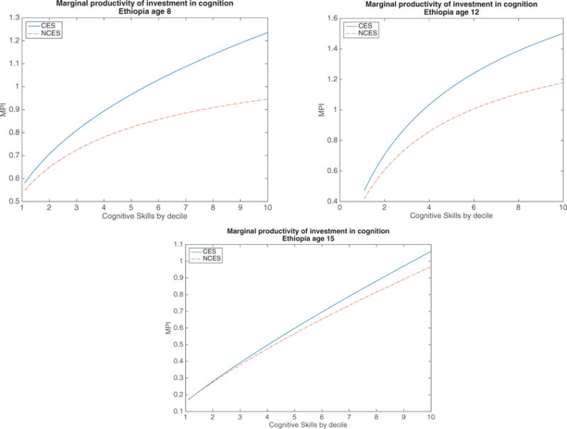
Marginal Product of Investment in Ethiopia

Figure 5.2.

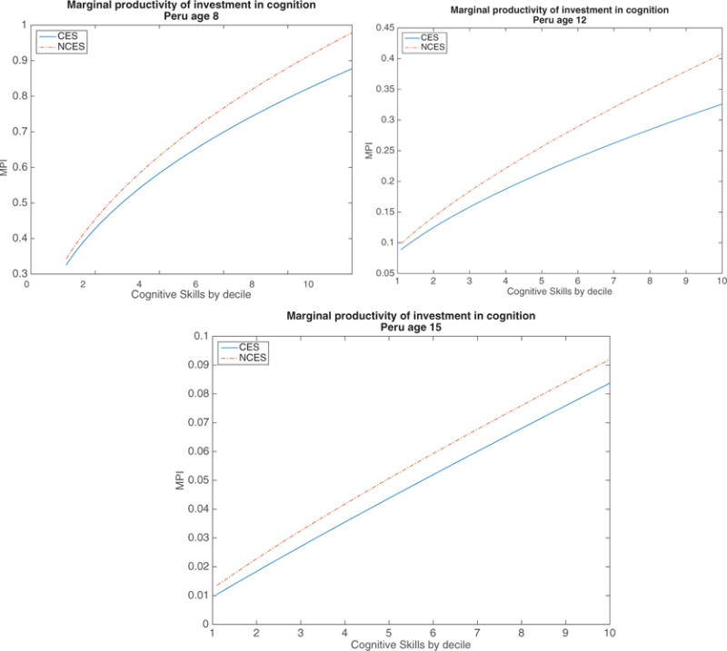
Marginal Product of Investment in Peru

6. Counterfactual Simulations

6.1. Impulse response functions

An important advantage of the longitudinal data we are using is that they allow us to follow children over a long period of time and estimate in a flexible way the degree of persistence and cross productivity of shocks and inputs. One way to study the implications of our sets of parameter estimates is to plot an impulse response function for investment innovations. In this subsection, we present this exercise for Ethiopia and Peru in Figures 6.1 and 6.2.

Figure 6.1.

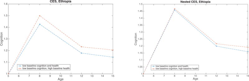
Figure 6.2.

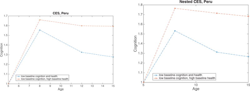
The experiment we perform is to select the children who are, at age 5, in the bottom 5% in terms of cognition. Using this sample, we compute the median values for all inputs and skills, including cognition. As one would expect, children who are “poor” in terms of cognitive skills, also have poorer health, poorer parental health and poorer parental cognition. Using these values and our estimates of the production functions we can predict the pattern of cognition that would occur for this sample (according to our model) if no changes were made. This is our baseline. In Figures 6.1 and 6.2 below, we plot the pattern of cognition that would occur, according to the model, in two alternative scenarios about parental inputs and initial health conditions, relative to the baseline. In the first scenario, we increase the investments these children receive at age 5 to equal the median investment of children in the top 10% in terms of cognition, and then follow the effect of the increase in investments through age 15 as implied by the production functions we have estimated. In the second scenario, we repeat the exercise but also give the child an initial health level at age 5 equivalent to the median health level of children in the top 10% of cognition at that age. This exercise is meant to capture the effect of increasing both inputs in the presence of dynamic complementarities. Any outcome in the figures above 1 implies an increase in cognition relative to the status quo.

For both countries and both production functions we observe that a positive shock to investment and health, as well as to investments alone, have large positive effects on the evolution of cognition over time. Specifically, the interventions lead to a 15–70% increase in cognition by age 15. For Ethiopia, increasing both investment and health at baseline leads to a larger increase in cognition at age 8 in the CES specification compared to the nested CES case, although by age 15 the differences between the two specifications are less noticeable. While there is a small gain from increasing both health and investments versus investments alone in the CES case for Ethiopia, for the nested CES specification the increase in later cognition due to the two alternative policies is almost identical. In Peru the difference between the two interventions is larger, with greater gains from increasing both health and investments at baseline. This result signifies greater levels of complementarity in Peru. This effect is somewhat larger with the nested CES. The key point demonstrated by these exercises is that the complementarity between initial conditions and investments can lead to substantially different results. Moreover, this exercise emphasizes the importance of health at an early age: with low health levels child outcomes respond less to investments.

6.2. Quantifying the importance of parental investments in generating inequality in child outcomes

In this section, we compare the patterns of cognitive skills over time for children who have the same baseline initial skill levels, but whose parents belong to different ends of the income distribution. First, we assign children the median level of skills in our sample, as well as the median amount of all other inputs. Next, we use our estimates of the investment equation to compute parental investments for children whose parents are at the 90th income percentile in our data, and the same investments for children whose parents are at the 10th income percentile in our data (all else equal). We then compute the evolution of cognitive skills over childhood for these two different patterns of investment. After the initial age, investments at later ages are also computed using our investment function estimates. However, at later ages not only will children receive different investments due to the differences in their parent’s incomes, but also as a result of the differences in cognition and health that come out of the production functions via inequality in investments accumulated in previous ages. The results from this exercise are reported in Figure 6.3. The dashed line shows the evolution of cognitive skills over time when parental investment is computed using the 90th percentile of income in our data. The dot-dashed line shows the same pattern for investment computed using the 10th percentile of income in our data. Both these lines are relative to the outcome that would occur if median income was used. In addition, we include two more lines. These lines show the evolution of skills when initial conditions are not restricted to be the same. Instead, for the top line, we compute the evolution of skills for children whose parents are at the 90th income percentile AND who have the corresponding top 10 percentile level of initial skills (cognition and health), relative to the median. The bottom line gives the evolution of skills for children whose parents are at the 10th income percentile AND who have the corresponding bottom 10 percentile level of initial skills. To economize on space we just show the results for the nested CES. These graphs clearly show that children of high income families, who enjoy persistently higher levels of parental investments, immediately open a large gap relative to poorer children, and this gap not only persists over time but grows. This is despite the same initial conditions and illustrates the inequalities that arise simply from different investments among the better off and the poorer. What is even more impressive is that while the initial gap in skills is much larger at age 5 when initial skills correspond to the income percentile (which is mechanically expected when compared to the case where initial skills are required to be equal) a substantial part of the gap that persists to age 15 when initial conditions are allowed to differ appears to be consistent with the gaps driven by differences in parental income which drive differences in investments at early ages.

Figure 6.3.

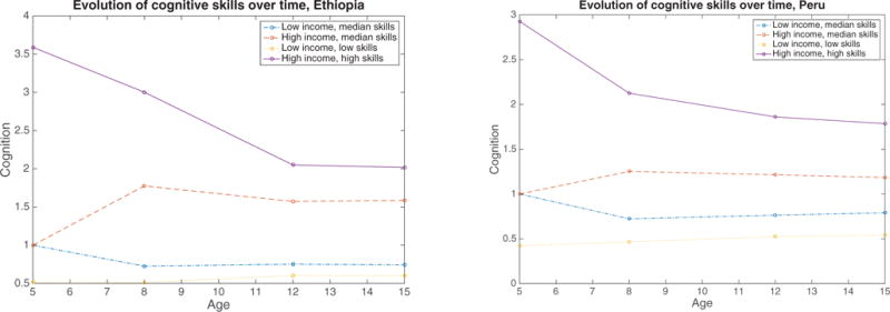
7. Conclusion

Understanding the development of human capital from an early age is critical to tracing the origins of inequality, to understanding the mechanisms for the inter-generational transmission of skills, and ultimately to design policies that can reduce poverty in a substantial way.

In this paper, following the approach of Cunha, Heckman, and Schennach (2010) and building on work for Colombia and India (Attanasio, Cattan, Fitzsimons et al. (2015) and Attanasio, Meghir, and Nix (2015), respectively) we estimate the determinants of investments in children and how these affect child outcomes in Peru and Ethiopia. Relative to previous studies we investigate the implications of more flexible functional forms that allow for richer patterns of complementarities among different inputs of the production function and add to the evidence by bringing in data from other developing countries, which helps identify common patterns.

We show that in several contexts, allowing for a flexible functional form is important. While in some cases the relatively simple Constant Elasticity of Substitution production function performs well, we find that in many cases the more flexible patterns of complementarity across different inputs allowed by a Nested CES fit the data better. This has important implications for the interpretation of the results, and we show that the shape of the marginal productivity of investments by decile of cognitive skills can be quite different for the CES and Nested CES.

Our focus is on cognition and health, for which we have rich information in the Young Lives Survey. While there are some important differences in the results from the two countries, some common elements stand out, which are also consistent with earlier work. First, investments increase with parental cognition and income, implying that children from better backgrounds get more resources and those resources may also be used more effectively. While this result is not unexpected, the large differences in cognitive development we document driven only by differences in parental income clearly illustrates that this may be an important source of social inequality and points to the potential importance of interventions boosting investments in children from poor backgrounds at a very early stage.

Second, cognition and health are self productive, implying persistence of past levels of child skills. However, there is some depreciation of skills, particularly at the cognitive level, which points to the potential importance of continuing investments throughout childhood. Third, health is important for cognitive development, a result that is similar to what is found for India by Attanasio, Meghir, and Nix (2015). This is a key result because poor health at early ages is prevalent in developing countries. Our results confirm that such ill-health can cause cognitive deficits, starting at very young ages, which can perpetuate poverty. Fourth, investments are important for cognition; however for both countries their impact declines with age pointing to the importance of early interventions. This result coupled with the fact that the elasticity of investments with respect to income is higher at lower ages points to another source of inequality, since the poor will tend to invest less exactly when such investments are most important. Finally, inputs into the production of human capital are complementary, at least based on the measurements and normalizations used in this paper, and the nested CES, which implies richer patterns of complementarity, generally fits the data better.

Together, these results provide important evidence that it is key to devise and implement health and cognition interventions that account for their complex interactions over childhood in order to promote human development. For example, programs focused on cognitive stimulation, sanitation, and possibly nutrition at very early ages can have long lasting and mutually reinforcing effects. We expect our results to further stimulate experimentation with such interventions. In addition, future work could extend the work done in this paper to additional contexts, and connect skills at adulthood to interesting adult outcomes like completed schooling, criminality, and wages, in order to better understand the mapping from these important skills to other policy relevant outcomes.

Appendix A. Summary Statistics

Table 12.

Summary Statistics: Child Measurements Ethiopia

	Younger Cohort			Older Cohort
	Age 1	Age 5	Age 8	Age 8	Age 12	Age 15
Gender (male)	0.53	0.53	0.53	0.51	0.51	0.51
Health Measures
Height for Age Z-Score	−1.58 (1.96)	−1.45 (1.13)	−1.21 (1.07)	−1.48 (1.29)	−1.39 (1.27)	−1.37 (1.29)
Weight for Age Z-Score	−1.43 (1.52)	−1.36 (0.93)	−1.63 (0.94)	−2.03 (1.34)	. .	. .
Weight in kg	7.96 (1.47)	15.68 (2.02)	20.49 (2.89)	19.13 (3.37)	30.37 (5.83)	40.47 (8.07)
How is Child’s Health? (0–2)	1.86 (0.78)	1.55 (0.66)	. .	1.23 (0.68)	1.23 (0.62)	. .
How is Child’s Health? (1–5)	. .	. .	4 (0.87)	. .	. .	4.04 (0.86)
Cognitive Measures
Number Correct PPVT Test	. .	21.42 (12.39)	68.35 (36.77)	. .	75.87 (26.16)	124.27 (28.36)
Rasch Score Math Test	. .	. .	300 (14.99)	. .	300.00 (49.94)	300.00 (14.98)
Rasch Score CDA Test	. .	300 (49.97)	. .	. .	. .	. .
Rasch Score Egra Test	. .	. .	300 (14.99)	. .	. .	. .
Rasch Score Cloze Test	. .	. .	. .	. .	. .	300.00 (14.98)
Ravens Total Correct (0–36)	. .	. .	. .	16.79 (6.31)	. .	. .
Child’s Reading Level (1–4)	. .	. .	. .	1.94 (1.20)	3.26 (1.04)	. .
Child’s Writing Level (0–2)	. .	. .	. .	0.66 (0.83)	1.21 (0.63)	. .
What is 2×4? (1 if correct)	.	.	.	0.44	.	.
Observations		1,999			1000

Table 13.

Summary Statistics: Child Measurements Peru

	Younger Cohort			Older Cohort
	Age 1	Age 5	Age 8	Age 8	Age 12	Age 15
Gender (male)	0.50	0.50	0.50	0.54	0.54	0.54
Health Measures
Height for Age Z-Score	−1.30 (1.36)	−1.56 (1.16)	−1.17 (1.06)	−1.41 (1.01)	−1.53 (1.15)	−1.48 (0.90)
Weight for Age Z-Score	−0.20 (1.21)	−0.54 (1.25)	−0.34 (1.20)	−0.50 (0.96)	. .	. .
Weight in kg	9.10 (1.42)	17.84 (3.02)	24.46 (4.96)	23.74 (3.67)	38.60 (8.57)	50.40 (8.82)
How is Child’s Health? (0–2)	1.26 (0.68)	1.03 (0.58)	. .	1.22 (0.62)	1.23 (0.57)	. .
How is Child’s Health? (1–5)	. .	. .	3.71 (0.65)	. .	. .	3.75 (0.67)
Cognitive Measures
Rasch Score PPVT Test	. .	300.00 (50.00)	300.00 (15.01)	. .	300.00 (50.00)	300.00 (15.00)
Rasch Score Math Test	. .	. .	300.03 (14.98)	. .	300.00 (50.00)	300.00 (15.00)
Rasch Score CDA Test	. .	300.00 (49.99)	. .	. .	. .	. .
Rasch Score Egra Test	. .	. .	300.01 (15.01)	. .	. .	. .
Rasch Score Cloze Test	. .	. .	. .	. .	. .	300.00 (15.00)
Ravens Total Correct (0–36)	. .	. .	. .	20.82 (8.06)	. .	. .
Child’s Reading Level (1–4)	. .	. .	. .	3.59 (0.96)	3.93 (0.39)	. .
Child’s Writing Level (0–2)	. .	. .	. .	1.42 (0.71)	1.12 (0.36)	. .
What is 2×4? (1 if correct)	.	.	.	0.75	.	.
Observations		2,052			714

Appendix B. Estimates of the nested CES for health at Age 8 for Peru and Age 12 for Ethiopia

Table 14.

Production of Human Capital, Nested CES Production Function, Health

	Health
	Peru, Age 8	Ethiopia, Age 12
Cognition	−0.046 [−0.09,−0.01]	0.201 [0.11,0.24]
Health	1.046 [1.01,1.09]	0.799 [0.76,0.89]
Parental Cognition	0.019 [−0.04,0.04]	−0.089 [−0.13,0]
Parental Health	−0.047 [−0.07,0.01]	0.043 [0,0.09]
Investment	−0.012 [−0.08,0.1]	−0.125 [−0.26,0.07]
Coefficient on Nested Skills	1.04 [0.93,1.09]	1.17 [0.98,1.27]
Complementarity (ρ)	0.025 [−0.78,0.56]	−0.045 [−0.41,0.3]
Elasticity of Substitution	1.026 [0.55,2.12]	0.957 [0.71,1.43]
Complementarity Nested (ρskills)	−0.055 [−0.42,0.14]	0.735 [0.43,1.08]
Elasticity of Substitution Nested	0.948 [0.7,1.14]	3.771 [−11.96,11.06]
log TFP (log(At))	0.017 [0.01,0.04]	−0.023 [−0.07,0.02]
Investment Residual (υ)	0.019 [−0.1,0.13]	0.254 [−0.24,0.48]
Number of Children	−0.017 [−0.03,0]	−0.004 [−0.02,0.01]
Older Siblings	0.013 [0,0.03]	−0.011 [−0.02,0.02]
Gender	−0.007 [−0.02,0]	−0.01 [−0.02,0.01]

Notes: 95% confidence intervals based on 100 bootstrap replications in square brackets.

Appendix C. Estimates without Instruments for Investments

Table 15.

Production of Human Capital, CES Production Function, Ethiopia

	Cognition				Health
Age	5	8	12	15	5	8	12	15
Cognition		0.438 [0.32,0.54]	0.502 [0.37,0.6]	0.871 [0.7,0.93]		0.015 [−0.03,0.05]	0.237 [0.13,0.29]	0.051 [−0.02,0.12]
Health	0.215 [0.13,0.26]	0.145 [0.08,0.21]	0.101 [0.02,0.22]	0.048 [0,0.1]	0.635 [0.56,0.68]	1.009 [0.94,1.05]	0.865 [0.81,0.96]	0.885 [0.82,0.93]
Parental Cognition	0.314 [0.22,0.41]	0.103 [0.05,0.19]	0.051 [0.02,0.12]	0.009 [−0.04,0.07]	0.014 [−0.04,0.06]	0.019 [−0.03,0.05]	−0.063 [−0.11,0]	0 [−0.05,0.03]
Parental Health	0.087 [0.04,0.16]	−0.002 [−0.04,0.04]	−0.007 [−0.03,0.03]	−0.003 [−0.03,0.04]	0.17 [0.13,0.29]	−0.009 [−0.02,0.02]	0.022 [−0.01,0.07]	0.04 [0.01,0.07]
Investment	0.383 [0.21,0.56]	0.316 [0.2,0.43]	0.353 [0.23,0.47]	0.075 [0,0.24]	0.181 [0.08,0.24]	−0.035 [−0.1,0.05]	−0.06 [−0.2,0.06]	0.024 [−0.06,0.11]
Complementarity (ρ)	−0.278 [−0.52,0.06]	0.013 [−0.18,0.46 ]	−0.514 [−0.71,−0.1]	−0.186 [−0.42,0.62]	−0.365 [−0.44,−0.12]	−0.094 [−0.5,0.52]	0.516 [0.34,0.89]	−0.435 [−0.74,0.16]
Elasticity of Substitution	0.783 [0.66,1.06]	1.014 [0.85,1.85]	0.661 [0.59,0.91]	0.843 [0.71,2.62]	0.732 [0.69,0.89]	0.914 [0.67,2.07]	2.068 [1.47,5.85]	0.697 [0.58,1.19]
log TFP (log(At))	0.026 [−0.05,0.05]	0.013 [−0.03,0.04]	0.019 [−0.06,0.07]	−0.05 [−0.13,−0.02]	0.081 [0.03,0.12]	0.001 [−0.03,0.02]	0.012 [−0.05,0.05]	0.13 [0.1,0.18]
Number of Children	−0.024 [−0.05,0]	−0.025 [−0.05,−0.01]	0.028 [0.01,0.06]	−0.027 [−0.05,−0.01]	−0.048 [−0.09,−0.03]	−0.004 [−0.03,0.01]	−0.004 [−0.02,0.01]	0.001 [−0.01,0.02]
Older Siblings	0.027 [0.01,0.06]	0.016 [0,0.04]	−0.017 [−0.05,0.01]	0.015 [0,0.05]	0.027 [0.01,0.07]	0.012 [0,0.04]	−0.008 [−0.02,0.02]	0.005 [0,0.02]
Gender	0.013 [0,0.02]	0 [−0.01,0.01]	0.009 [−0.01,0.03]	0.044 [0.02,0.07]	0.001 [−0.01,0.01]	−0.007 [−0.02,0]	−0.011 [−0.02,0.01]	−0.071 [−0.09,−0.06]

Notes: 95% confidence intervals based on 100 bootstrap replications in square brackets.

Table 16.

Production of Human Capital, CES Production Function, Peru

	Cognition				Health
Age	5	8	12	15	5	8	12	15
Cognition		0.497 [0.41,0.62]	0.694 [0.5,0.77]	0.861 [0.49,0.95]		−0.05 [−0.07,−0.02]	−0.039 [−0.1,0.05]	−0.036 [−0.08,0.02]
Health	0.115 [0.01,0.15]	0.078 [0.01,0.14]	0.091 [0.02,0.17]	0.037 [−0.02,0.17]	0.684 [0.63,0.73]	1.086 [1.01,1.11]	0.988 [0.88,1.03]	0.954 [0.86,0.99]
Parental Cognition	0.479 [0.37,0.64]	0.272 [0.18,0.37]	0.316 [0.17,0.37]	0.086 [0.05,0.38]	0.055 [0.01,0.11]	0.014 [−0.02,0.03]	0.078 [0,0.12]	0.022 [−0.03,0.07]
Parental Health	0.17 [0.03,0.29]	0.007 [−0.08,0.08]	−0.065 [−0.19,0.03]	−0.036 [−0.16,0.02]	0.185 [0.11,0.24]	−0.051 [−0.08,0.01]	0.008 [−0.06,0.09]	0.077 [0.02,0.17]
Investment	0.236 [0.14,0.41]	0.146 [0.07,0.22]	−0.036 [−0.09,0.25]	0.052 [−0.05,0.16]	0.076 [0.02,0.14]	0.001 [−0.02,0.06]	−0.036 [−0.1,0.08]	−0.016 [−0.07,0.05]
Complementarity (ρ)	0.141 [−0.06,1.56]	0.069 [−0.11,0.22]	0.205 [−0.06,0.48]	−0.036 [−0.48,0.25]	−0.001 [−0.18,0.18]	0.011 [−0.23,0.29]	0.14 [−0.25,0.42]	−0.334 [−0.82,0.24]
Elasticity of Substitution	1.164 [−1.94,4.34]	1.074 [0.9,1.28]	1.259 [0.94,1.95]	0.966 [0.68,1.33]	0.999 [0.85,1.23]	1.012 [0.81,1.41]	1.163 [0.8,1.73]	0.75 [0.55,1.32]
log TFP (log(At))	−0.069 [−0.15,−] 0.04	−0.031 [−0.06,0]	0.051 [−0.01,0.11]	−0.068 [−0.11,−0.03]	−0.022 [−0.05,0]	0.018 [0.01,0.04]	−0.037 [−0.07,0]	−0.099 [−0.12,−0.07]
Number of Children	0.019 [−0.01,0.03]	−0.019 [−0.05,0]	−0.037 [−0.07,−0.01]	0.007 [−0.02,0.02]	−0.012 [−0.02,0]	−0.017 [−0.03,0]	−0.013 [−0.03,0]	0.02 [0,0.03]
Older Siblings	−0.002 [−0.01,0.03]	0.021 [0,0.05]	0 [−0.03,0.02]	0.02 [0,0.05]	0.002 [−0.02,0.01]	0.013 [0,0.03]	0.025 [0.01,0.04]	−0.007 [−0.02,0.01]
Gender	0.011 [0,0.03]	0.015 [0,0.02]	0.001 [−0.02,0.03]	0.013 [0,0.04]	0.022 [0.01,0.03]	−0.007 [−0.02,0]	0.009 [−0.01,0.02]	0.046 [0.03,0.06]

Notes: 95% confidence intervals based on 100 bootstrap replications in square brackets.

Table 17.

Production of Human Capital, Nested CES Production Function, Ethiopia

	Cognition			Health
Age	8	12	15	8	12	15
Cognition	0.827 [0.7,0.95]	0.882 [0.68,0.99]	0.949 [0.88,0.99]	0.015 [−0.03,0.05]	0.19 [0.1,0.23]	0.06 [−0.02,0.13]
Health	0.173 [0.05,0.3]	0.118 [0.01,0.32]	0.051 [0.01,0.12]	0.985 [0.95,1.03]	0.81 [0.77,0.9]	0.94 [0.87,1.02]
Parental Cognition	0.084 [0.05,0.16]	0.054 [0.02,0.12]	0.01 [−0.04,0.07]	0.018 [−0.03,0.05]	−0.106 [−0.15,−0.01]	0.003 [−0.04,0.03]
Parental Health	0.006 [−0.03,0.03]	−0.008 [−0.04,0.03]	−0.004 [−0.03,0.04]	−0.009 [−0.02,0.02]	0.033 [−0.01,0.09]	0.021 [0,0.07]
Investment	0.292 [0.15,0.4]	0.369 [0.25,0.47]	0.076 [0.01,0.24]	−0.035 [−0.09,0.05]	−0.053 [−0.19,0.06]	0.021 [−0.06,0.11]
Coefficient on Nested Skills	0.618 [0.52,0.74]	0.586 [0.47,0.69]	0.919 [0.77,0.97]	1.025 [0.94,1.07]	1.126 [0.99,1.2]	0.955 [0.87,1.02]
Complementarity (ρ)	0.618 [0.22,1.2]	−0.2 [−0.59,0.24]	−0.027 [−0.55,1.39]	−0.156 [−0.64,0.66]	−0.064 [−0.49,0.31]	−0.898 [−1.1,0.34]
Elasticity of Substitution	2.617 [−5.66,6.6]	0.833 [0.63,1.31]	0.974 [−1.95,2.38]	0.865 [0.55,2.55]	0.94 [0.66,1.38]	0.527 [0.47,1.43]
Complementarity Nested (ρskills)	−1.149 [−2.56,−] 0.39	−1.204 [−2.29,−0.33]	−0.322 [−0.47,0.21]	0.088 [−1.15,0.72]	0.841 [0.52,1.13]	0.28 [−1.12,0.96]
Elasticity of Substitution Nested	0.465 [0.28,0.72]	0.454 [0.3,0.75]	0.756 [0.61,1.25]	1.097 [0.47,3.69]	6.285 [−8.71,18.75]	1.389 [0.32,7.32]
log TFP (log(At))	0.018 [−0.03,0.05]	0.018 [−0.06,0.07]	−0.05 [−0.12,−0.02]	−0.001 [−0.03,0.02]	−0.02 [−0.07,0.03]	0.125 [0.1,0.17]
Number of Children	−0.023 [−0.05,0]	0.027 [0.01,0.06]	−0.027 [−0.05,−0.01]	−0.004 [−0.03,0.01]	−0.008 [−0.03,0.01]	0.002 [−0.01,0.02]
Older Siblings	0.015 [ 0,0.04]	−0.017 [−0.05,0.01]	0.015 [0,0.05]	0.012 [0,0.04]	−0.01 [−0.02,0.02]	0.005 [0,0.02]
Gender	0 [−0.01,0.01]	0.009 [−0.01,0.03]	0.044 [0.02,0.07]	−0.007 [−0.01,0]	−0.011 [−0.02,0.01]	−0.071 [−0.09,−0.06]

Notes: 95% confidence intervals based on 100 bootstrap replications in square brackets.

Table 18.

Production of Human Capital, Nested CES Production Function, Peru

	Cognition			Health
Age	8	12	15	8	12	15
Cognition	0.866 [0.76,0.97]	0.892 [0.76,0.98]	0.965 [0.75,1.02]	−0.05 [−0.07,−0.02]	−0.04 [−0.11,0.05]	−0.035 [−0.09,0.03]
Health	0.134 [0.03,0.24]	0.108 [0.02,0.24]	0.035 [−0.02,0.25]	1.05 [1.02,1.07]	1.04 [0.95,1.11]	1.035 [0.97,1.09]
Parental Cognition	0.271 [0.18,0.37]	0.317 [0.17,0.37]	0.083 [0.05,0.38]	0.014 [−0.02,0.03]	0.078 [0,0.12]	0.023 [−0.03,0.07]
Parental Health	0.008 [−0.09,0.09]	−0.065 [−0.19,0.03]	−0.034 [−0.16,0.02]	−0.051 [−0.08,0.01]	0.008 [−0.06,0.08]	0.08 [0.02,0.17]
Investment	0.146 [0.07,0.22]	−0.032 [−0.08,0.25]	0.055 [−0.05,0.16]	0.003 [−0.02,0.06]	−0.036 [−0.09,0.08]	−0.02 [−0.07,0.05]
Coefficient on Nested Skills	0.575 [0.49,0.69]	0.781 [0.57,0.88]	0.895 [0.61,0.99]	1.034 [0.96,1.07]	0.95 [0.85,1.03]	0.918 [0.83,0.97]
Complementarity (ρ)	0.049 [−0.13,0.28]	0.17 [−0.08,0.4]	0.165 [−0.84,0.31]	0.186 [−0.6,0.76]	0.136 [−0.32,0.61]	−0.252 [−0.83,0.24]
Elasticity of Substitution	1.051 [0.89,1.38]	1.205 [0.92,1.68]	1.198 [0.54,1.46]	1.228 [0.62,4.3]	1.158 [0.76,2.59]	0.799 [0.54,1.29]
Complementarity Nested (ρskills)	0.176 [−0.4,0.61]	0.488 [−0.09,1.76]	−0.534 [−0.79,0.61]	−0.053 [−0.35,0.11]	0.188 [−1.1,1.03]	−0.495 [−1.03,0.54]
Elasticity of Substitution Nested	1.213 [0.71,2.57]	1.954 [−10.49,10.24]	0.652 [0.49,1.59]	0.95 [0.74,1.12]	1.231 [−0.39,2.23]	0.669 [0.49,2.17]
log TFP (log(At))	−0.032 [−0.06,0]	0.046 [−0.01,0.11 ]	−0.066 [−0.11,−0.03]	0.018 [0.01,0.04]	−0.036 [−0.07,0]	−0.102 [−0.12,−0.06]
Number of Children	−0.019 [−0.05,0]	−0.037 [−0.07,−0.01]	0.006 [−0.02,0.02]	−0.017 [−0.03,0]	−0.013 [−0.03,0]	0.02 [0,0.03]
Older Siblings	0.021 [0,0.05]	0 [−0.03,0.02]	0.02 [0,0.05]	0.013 [0,0.03]	0.025 [0.01,0.04]	−0.007 [−0.02,0.01]
Gender	0.015 [0,0.02]	0.001 [−0.02,0.03]	0.013 [0,0.04]	−0.007 [−0.02,0]	0.009 [−0.01,0.02]	0.046 [0.03,0.06]

Notes: 95% confidence intervals based on 100 bootstrap replications in square brackets.

Appendix D. Estimates Using Only Prices as Instruments

Table 19.

Production of Human Capital, CES Production Function, Ethiopia

	Cognition				Health
Age	5	8	12	15	5	8	12	15
Cognition		0.353 [0.26,0.45]	0.445 [0.32,0.55]	0.79 [0.56,0.86]		−0.001 [−0.05,0.04]	0.266 [0.13,0.34]	0.016 [−0.08,0.11]
Health	0.034 [−0.01,0.13]	0.093 [0.05,0.16]	0.039 [−0.03,0.13]	0.034 [−0.01,0.08]	0.547 [0.49,0.61]	1.007 [0.92,1.06]	0.895 [0.81,0.98]	0.872 [0.79,0.91]
Parental Cognition	0.064 [−0.05,0.17]	−0.054 [−0.07,0.06]	0.006 [−0.06,0.06]	−0.029 [−0.09,0.03]	−0.097 [−0.17,−0.01]	−0.033 [−0.08,0]	−0.038 [−0.1,0.01]	−0.011 [−0.07,0.02]
Parental Health	−0.015 [ ]−0.05,0.04	−0.051 [−0.1,−0.01]	−0.02 [−0.07,0.01]	−0.021 [−0.05,0.03]	0.122 [0.09,0.23]	−0.018 [−0.03,0.01]	0.042 [0,0.08]	0.029 [0,0.07]
Investment	0.917 [0.68,1.04]	0.659 [0.5,0.75]	0.531 [0.42,0.75]	0.225 [0.11,0.5]	0.429 [0.26,0.53]	0.045 [−0.05,0.16]	−0.165 [−0.31,0.02]	0.094 [−0.04,0.22]
Complementarity (ρ)	0.559 [−0.65,1.08]	−0.042 [−0.15,0.17]	−0.531 [−0.82,−0.09]	−0.04 [−0.31,0.35]	−0.2 [−0.26,−0.02]	0.077 [−0.31,0.42]	0.443 [0.24,0.9]	−0.49 [−0.71,0.17]
Elasticity of Substitution	2.269 [−8.34,7.89]	0.959 [0.87,1.2]	0.653 [0.55,0.91]	0.962 [0.76,1.55]	0.834 [0.8,0.98]	1.084 [0.75,1.52]	1.796 [1.2,6.24]	0.671 [0.59,1.2]
Log TFP	0.182 [−0.02,0.26]	−0.11 [−0.21,0.02]	−0.008 [−0.13,0.06]	−0.1 [−0.25,0]	0.187 [0.06,0.25]	−0.076 [−0.13,−0.04]	0.049 [−0.06,0.12]	0.151 [0.09,0.2]
Investment Residual (υ)	−0.784 [−0.91,−0.54]	−0.656 [−0.76,−0.48]	−0.525 [−0.84,−0.24]	−0.243 [−0.61,−0.08]	−0.361 [−0.49,−0.2]	−0.138 [−0.25,−0.01]	0.295 [−0.18,0.55]	−0.157 [−0.36,0.14]
Number of Children	−0.016 [−0.06,0.01]	−0.044 [−0.08,−0.02]	0.016 [0,0.05]	−0.028 [−0.05,0]	−0.048 [−0.1,−0.03]	−0.006 [−0.03,0.01]	−0.007 [−0.03,0.01]	−0.001 [−0.01,0.01]
Older Siblings	0.017 [0,0.06]	0.018 [0,0.05]	−0.013 [−0.05,0.01]	0.019 [−0.01,0.04]	0.024 [0.01,0.07]	0.011 [0,0.03]	0.001 [−0.02,0.02]	0.004 [−0.01,0.02]
Gender	−0.006 [−0.01,0.01]	0.004 [−0.01,0.02]	0.006 [−0.01,0.03]	0.044 [0.03,0.07]	−0.007 [−0.02,0]	−0.006 [−0.01,0]	−0.007 [−0.02,0.01]	−0.074 [−0.1,−0.06]
Income	−0.144 [−0.22,0]	0.124 [0.01,0.21]	0.028 [−0.05,0.09]	0.037 [−0.03,0.16]	−0.091 [−0.14,−0.01]	0.068 [0.04,0.11]	−0.038 [−0.09,0.05]	−0.006 [−0.06,0.04]

Notes: 95% confidence intervals based on 100 bootstrap replications in square brackets.

Table 20.

Production of Human Capital, CES Production Function, Peru

	Cognition				Health
Age	5	8	12	15	5	8	12	15
Cognition		0.457 [0.36,0.59]	0.681 [0.46,0.75]	0.875 [0.48,0.96]		−0.062 [−0.1,−0.02]	−0.027 [−0.1,0.08]	−0.023 [−0.08,0.04]
Health	0.041 [−0.05,0.12]	0.045 [−0.03,0.11]	0.004 [−0.09,0.12]	0.044 [−0.01,0.17]	0.702 [0.64,0.76]	1.089 [1.01,1.12]	0.964 [0.85,1.01]	0.975 [0.88,1.02]
Parental Cognition	−0.063 [−0.17,0.12]	0.207 [0.1,0.3]	0.093 [−0.01,0.24]	0.103 [0.04,0.36]	0.008 [−0.06,0.07]	−0.01 [−0.06,0.02]	0.006 [−0.08,0.06]	0.062 [0,0.13]
Parental Health	−0.064 [−0.19,0.08]	−0.086 [−0.18,−0.01]	−0.08 [−0.27,0.03]	−0.021 [−0.15,0.04]	0.21 [0.15,0.27]	−0.023 [−0.04,0.03]	0.01 [−0.06,0.08]	0.054 [0.01,0.13]
Investment	1.086 [0.8,1.25]	0.377 [0.24,0.54]	0.302 [0.14,0.53]	−0.002 [−0.09,0.19]	0.08 [−0.03,0.19]	0.007 [−0.05,0.11]	0.046 [−0.05,0.2]	−0.067 [−0.17,0.04]
Complementarity (ρ)	−0.294 [−0.97,0.76]	0.015 [ 0.1,0.17−]	−0.196 [ 0.45,0.19−]	−0.183 [−0.48,0.7]	−0.039 [−0.19,0.15]	−0.003 [−0.23,0.14]	−0.416 [−0.37,0.29]	0.264 [−0.86,0.42]
Elasticity of Substitution	0.773 [0.5,1.44]	1.015 [0.91,1.21]	0.836 [0.69,1.24]	0.845 [0.62,2]	0.963 [0.84,1.17]	0.997 [0.82,1.16]	0.706 [0.73,1.4]	1.359 [0.54,1.73]
Log TFP	−0.238 [−0.38,−0.1]	0.059 [−0.08,0.1]	−0.262 [−0.36,−0.04]	−0.051 [−0.22,0]	−0.159 [−0.24,−0.11]	−0.08 [−0.11,−0.01]	−0.152 [−0.23,−0.08]	0.01 [−0.05,0.1]
Investment Residual (υ)	−1.125 [−1.27,−0.84]	−0.323 [−0.51,−0.19]	−0.663 [−0.9,−0.19]	0.124 [−0.22,0.31]	−0.021 [−0.12,0.11]	−0.013 [−0.11,0.1]	−0.117 [−0.34,0.05]	−0.021 [−0.14,0.2]
Number of Children	0.04 [0,0.06]	−0.021 [−0.05,0.01]	−0.031 [−0.06,0]	0.008 [−0.02,0.02]	−0.004 [−0.02,0.01]	−0.011 [−0.03,0]	−0.012 [−0.02,0.01]	0.02 [0,0.03]
Older Siblings	−0.02 [−0.03,0.01]	0.02 [0,0.04]	−0.015 [−0.04,0.01]	0.022 [0,0.05]	−0.003 [−0.03,0.01]	0.009 [0,0.02]	0.02 [0,0.03]	−0.006 [−0.01,0.02]
Gender	0.001 [−0.01,0.02]	0.015 [0,0.03]	0 [−0.02,0.03]	0.01 [0,0.04]	0.022 [0.01,0.03]	−0.007 [−0.02,0]	0.008 [−0.01,0.02]	0.043 [0.03,0.06]
Income	0.153 [0.06,0.3]	−0.065 [−0.1,0.04]	0.284 [0.08,0.38]	−0.012 [−0.05,0.12]	0.11 [0.07,0.16]	0.077 [0.03,0.1]	0.104 [0.06,0.16]	−0.087 [−0.16,−0.04]

Notes: 95% confidence intervals based on 100 bootstrap replications in square brackets.

Table 21.

Production of Human Capital, Nested CES Production Function, Ethiopia

	Cognition			Health
Age	8	12	15	8	12	15
Cognition	0.847 [0.69,0.98]	0.953 [0.76,1.07]	0.958 [0.9,1.02]	0 [−0.05,0.05]	0.211 [0.11,0.26]	0.033 [−0.09,0.11]
Health	0.153 [0.02,0.31]	0.047 [−0.07,0.24]	0.042 [−0.02,0.1]	1 [0.95,1.05]	0.789 [0.74,0.89]	0.967 [0.89,1.09]
Parental Cognition	−0.047 [−0.06,0.06]	0.006 [−0.06,0.06]	−0.029 [−0.09,0.03]	−0.033 [−0.08,0]	−0.057 [−0.12,0.01]	−0.005 [−0.07,0.02]
Parental Health	−0.045 [−0.1,0]	−0.023 [−0.07,0.01]	−0.021 [−0.05,0.03]	−0.018 [−0.03,0.01]	0.047 [0.01,0.1]	0.021 [0,0.07]
Investment	0.643 [0.47,0.73]	0.536 [0.42,0.73]	0.225 [0.11,0.49]	0.045 [−0.05,0.16]	−0.173 [−0.33,0.02]	0.072 [−0.07,0.22]
Coefficient on Nested Skills	0.45 [0.35,0.56]	0.481 [0.36,0.58]	0.825 [0.6,0.91]	1.007 [0.9,1.08]	1.184 [0.97,1.29]	0.912 [0.77,0.98]
Complementarity (ρ)	0.119 [−0.06,0.43]	−0.428 [−0.75,0]	−0.028 [−0.32,0.52]	0.079 [−0.33,0.53]	−0.29 [−0.44,0.27]	−0.717 [−1.12,0.42]
Elasticity of Substitution	1.135 [0.94,1.76]	0.7 [0.57,1]	0.973 [0.76,2.09]	1.086 [0.75,2.15]	0.775 [0.7,1.37]	0.583 [0.47,1.72]
Complementarity Nested (ρskills)	−0.957 [−3.11,−0.16]	−1.358 [−2.73,0.17]	−0.117 [−0.76,0.74]	−3.646 [−0.82,0.75]	0.724 [0.43,1.13]	0.616 [−1,1.21]
Elasticity of Substitution Nested	0.511 [0.24,0.86]	0.424 [0.27,1.21]	0.895 [0.42,1.48]	0.215 [0.51,2.61]	3.628 [−7.63,11.86]	2.607 [−3.73,4.63]
log TFP (log(At))	−0.09 [−0.21,0.04]	−0.003 [−0.13,0.07]	−0.1 [−0.24,0]	−0.076 [−0.13,−0.04]	0.007 [−0.08,0.09]	0.148 [0.09,0.2]
Investment Residual (υ)	−0.636 [−0.74,−0.44]	−0.514 [−0.79,−0.24]	−0.243 [−0.6,−0.07]	−0.138 [−0.25,−0.01]	0.296 [−0.2,0.54]	−0.143 [−0.36,0.12]
Number of Children	−0.043 [−0.07,−0.02]	0.016 [0,0.05]	−0.028 [−0.05,0]	−0.006 [−0.03,0.01]	−0.009 [−0.03,0.01]	−0.001 [−0.01,0.01]
Older Siblings	0.017 [0,0.05]	−0.013 [−0.05,0.01]	0.019 [−0.01,0.04]	0.011 [0,0.03]	0 [−0.02,0.02]	0.005 [−0.01,0.02]
Gender	0.004 [−0.01,0.02]	0.006 [−0.01,0.03]	0.044 [0.03,0.07]	−0.006 [−0.01,0]	−0.005 [−0.02,0.01]	−0.074 [−0.1,−0.06]
Income	0.123 [0.01,0.21]	0.027 [−0.05,0.09]	0.037 [−0.03,0.16]	0.068 [0.04,0.11]	−0.038 [−0.09,0.05]	−0.008 [−0.06,0.03]

Notes: 95% confidence intervals based on 100 bootstrap replications in square brackets.

Table 22.

Production of Human Capital, Nested CES Production Function, Peru

	Cognition			Health
Age	8	12	15	8	12	15
Cognition	0.917 [0.81,1.06]	0.993 [0.79,1.14]	0.952 [0.77,1.01]	−0.061 [−0.1,−0.02]	−0.031 [−0.11,0.08]	−0.025 [−0.09,0.05]
Health	0.083 [−0.06,0.19]	0.007 [−0.14,0.21]	0.048 [−0.01,0.23]	1.061 [1.02,1.1]	1.031 [0.92,1.11]	1.025 [0.95,1.09]
Parental Cognition	0.206 [0.1,0.3]	0.095 [−0.01,0.23]	0.103 [0.04,0.36]	−0.006 [−0.05,0.02]	0.006 [−0.08,0.06]	0.062 [0,0.13]
Parental Health	−0.085 [−0.18,−0.01]	−0.086 [−0.27,0.03]	−0.021 [−0.15,0.04]	−0.024 [−0.04,0.03]	0.011 [−0.06,0.08]	0.054 [0.01,0.13]
Investment	0.378 [0.24,0.54]	0.3 [0.14,0.53]	−0.003 [−0.09,0.19]	0.003 [−0.05,0.11]	0.046 [−0.05,0.2]	−0.067 [−0.17,0.04]
Coefficient on Nested Skills	0.502 [0.4,0.62]	0.691 [0.47,0.78]	0.92 [0.6,0.99]	1.027 [0.93,1.07]	0.937 [0.82,1.01]	0.952 [0.84,1.02]
Complementarity (ρ)	−0.015 [−0.14,0.16]	−0.189 [−0.42,0.16]	−0.209 [−0.51,0.78]	0.268 [−0.91,0.8]	−0.4 [−0.42,0.38 ]	0.26 [−0.89,0.43]
Elasticity of Substitution	0.986 [0.88,1.18]	0.841 [0.7,1.19]	0.827 [0.51,2.13]	1.366 [0.47,2.55]	0.714 [0.71,1.62]	1.351 [0.53,1.75]
Complementarity Nested (ρskills)	0.521 [−0.53,1.04]	1.809 [−1.14,1.28]	−0.133 [−1.37,0.54]	−0.025 [−0.31,0.12]	−0.179 [−0.94,0.76]	−0.232 [−0.88,0.77]
Elasticity of Substitution Nested	2.09 [−1.25,8.4]	−1.236 [−3.49,4.38]	0.883 [0.35,1.5]	0.975 [0.76,1.14]	0.848 [0.45,2.05]	0.812 [0.48,2.56]
log TFP (log(At))	0.054 [−0.08,0.1]	−0.265 [−0.37,−0.04]	−0.051 [−0.22,0]	−0.079 [−0.11,−0.01]	−0.151 [−0.23,−0.08]	0.005 [−0.06,0.1]
Investment Residual (υ)	−0.325 [−0.51,−0.18]	−0.661 [−0.9,−0.19]	0.126 [−0.22,0.31]	−0.01 [−0.11,0.1]	−0.116 [−0.34,0.05]	−0.02 [−0.14,0.2]
Number of Children	−0.021 [−0.05,0.01]	−0.03 [−0.06,0]	0.008 [−0.02,0.02]	−0.011 [−0.03,0]	−0.012 [−0.02,0.01]	0.02 [0,0.03]
Older Siblings	0.02 [0,0.04]	−0.015 [−0.04,0.01]	0.022 [0,0.05]	0.009 [0,0.02]	0.02 [0,0.03]	−0.006 [−0.01,0.02]
Gender	0.015 [0,0.03]	0 [−0.02,0.03]	0.01 [0,0.04]	−0.007 [−0.02,0]	0.008 [−0.01,0.02]	0.043 [0.03,0.06]
Income	−0.065 [−0.1,0.04]	0.281 [0.08,0.38]	−0.012 [−0.05,0.12]	0.076 [0.03,0.1]	0.104 [0.06,0.16]	−0.087 [−0.15,−0.04]

Notes: 95% confidence intervals based on 100 bootstrap replications in square brackets.

Appendix E. Estimates Using Prices, Income, and their Interactions as Instruments

Table 23.

Production of Human Capital, CES Production Function, Ethiopia

	Cognition				Health
Age	5	8	12	15	5	8	12	15
Cognition		0.374 [0.27,0.48]	0.472 [0.33,0.57]	0.813 [0.58,0.89]		0.008 [−0.04,0.05]	0.25 [0.13,0.3]	0.011 [−0.07,0.1]
Health	0.125 [0.05,0.21]	0.092 [0.04,0.17]	0.041 [−0.03,0.14]	0.045 [−0.01,0.08]	0.593 [0.53,0.64]	1.004 [0.92,1.05]	0.902 [0.81,0.97]	0.884 [0.81,0.92]
Parental Cognition	0.104 [0.02,0.25]	0.038 [−0.01,0.15]	0.012 [−0.03,0.09]	−0.004 [−0.07,0.06]	−0.08 [−0.15,0]	0.012 [−0.03,0.04]	−0.065 [−0.11,0]	−0.023 [−0.07,0.02]
Parental Health	0.015 [ 0.02,0.08−]	−0.032 [−0.07,0.01]	−0.022 [−0.07,0.02]	−0.021 [−0.05,0.03]	0.14 [0.11,0.25]	−0.012 [−0.02,0.02]	0.045 [0,0.08]	0.026 [0.01,0.07]
Investment	0.756 [0.51,0.91]	0.527 [0.33,0.63]	0.497 [0.38,0.71]	0.167 [0.06,0.43]	0.347 [0.18,0.45]	−0.011 [−0.09,0.11]	−0.132 [−0.25,0.05]	0.102 [−0.02,0.24]
Complementarity (ρ)	−0.519 [−0.83,0.37]	0.049 [−0.1,0.47]	−0.516 [−0.83,−0.1]	0.005 [−0.32,0.56]	−0.285 [−0.4,−0.06]	−0.122 [−0.59,0.55]	0.431 [0.26,0.98]	−0.583 [−0.64,0.06]
Elasticity of Substitution	0.658 [0.54,1.44]	1.052 [0.91,1.88]	0.659 [0.55,0.91]	1.005 [0.76,2.27]	0.778 [0.72,0.94]	0.891 [0.63,2.21]	1.756 [−0.16,3.71]	0.632 [0.61,1.07]
log TFP (log(At))	0.052 [−0.05,0.06]	0.028 [−0.02,0.05]	0.014 [−0.06,0.07]	−0.069 [−0.11,−0.01]	0.079 [0.04,0.11]	0.002 [−0.03,0.02]	0.012 [−0.05,0.04]	0.16 [0.1,0.17]
Investment Residual (υ)	−0.583 [−0.74,−0.33]	−0.517 [−0.65,−0.26]	−0.519 [−0.77,−0.22]	−0.157 [−0.52,−0.03]	−0.285 [−0.43,−0.14]	−0.06 [−0.18,0.03]	0.263 [−0.18,0.52]	−0.178 [−0.36,0.13]
Number of Children	−0.019 [−0.06,0.01]	−0.039 [−0.07,−0.02]	0.025 [0,0.05]	−0.031 [−0.05,−0.01 ]	−0.046 [−0.1,−0.03]	−0.005 [−0.03,0.01]	−0.014 [−0.03,0.01]	−0.002 [−0.02,0.01]
Older Siblings	0.02 [0,0.06]	0.018 [0,0.05]	−0.017 [−0.05,0.01]	0.024 [0,0.05]	0.024 [0.01,0.07]	0.012 [0,0.04]	0.001 [−0.02,0.02]	0.004 [−0.01,0.02]
Gender	0.002 [−0.01,0.02]	0.003 [−0.01,0.02]	0.006 [−0.01,0.03]	0.051 [0.03,0.07]	−0.004 [−0.02,0.01]	−0.007 [−0.02,0]	−0.007 [−0.02,0.01]	−0.082 [−0.09,−0.06]

Notes: 95% confidence intervals based on 100 bootstrap replications in square brackets.

Table 24.

Production of Human Capital, CES Production Function, Peru

	Cognition				Health
Age	5	8	12	15	5	8	12	15
Cognition		0.458 [0.36,0.59]	0.65 [0.44,0.74]	0.87 [0.49,0.96]		−0.048 [−0.08,−0.01]	−0.04 [−0.12,0.06]	−0.038 [−0.09,0.03]
Health	0.023 [−0.04,0.1]	0.054 [−0.02,0.11]	0.085 [0,0.16]	0.04 [−0.01,0.18]	0.681 [0.63,0.74]	1.088 [1.01,1.11]	0.988 [0.88,1.03]	0.954 [0.86,1]
Parental Cognition	0.025 [−0.08,0.25]	0.204 [0.12,0.3]	0.299 [0.13,0.37]	0.096 [0.06,0.38]	0.042 [−0.01,0.13]	0.018 [−0.03,0.04]	0.077 [−0.01,0.11]	0.007 [−0.02,0.08]
Parental Health	−0.079 [−0.22,0.06 ]	−0.047 [−0.15,0.03]	−0.102 [−0.27,0]	−0.02 [−0.15,0.03]	0.178 [0.11,0.24]	−0.047 [−0.07,0.01]	0.007 [−0.08,0.08]	0.053 [0.02,0.17]
Investment	1.031 [0.75,1.18]	0.331 [0.21,0.51]	0.067 [−0.07,0.43]	0.014 [−0.1,0.15]	0.098 [−0.04,0.2]	−0.011 [−0.08,0.1]	−0.033 [−0.12,0.16]	0.023 [−0.1,0.09]
Complementarity (ρ)	−0.421 [−0.76,1.03]	−0.018 [−0.15,0.17]	0.112 [−0.15,0.39]	−0.087 [−0.65,0.15]	0.011 [−0.22,0.18]	−0.023 [−0.29,0.21]	0.137 [−0.23,0.43]	−0.52 [−0.88,0.22]
Elasticity of Substitution	0.704 [−1,8.27]	0.982 [0.87,1.21]	1.127 [0.87,1.64]	0.92 [0.61,1.17]	1.011 [0.82,1.23]	0.978 [0.77,1.27]	1.159 [0.82,1.74]	0.658 [0.53,1.28]
log TFP (log(At))	−0.039 [−0.11,0]	−0.02 [−0.05,0.01]	0.051 [−0.01,0.11]	−0.068 [−0.11,−0.03]	−0.022 [−0.05,0]	0.017 [0.01,0.04]	−0.037 [−0.07,0]	−0.095 [−0.12,−0.06]
Investment Residual (υ)	−1.069 [−1.2,−0.75]	−0.272 [−0.47,−0.14]	−0.382 [−0.66,−0.01]	0.103 [−0.16,0.33]	−0.03 [−0.14,0.17]	0.017 [−0.1,0.13]	−0.011 [−0.22,0.16]	−0.123 [−0.21,0.12]
Number of Children	0.03 [−0.01,0.04]	−0.017 [−0.04,0.01]	−0.034 [−0.07,0]	0.008 [−0.02,0.02]	−0.011 [−0.02,0]	−0.017 [−0.03,0]	−0.013 [−0.03,0.01]	0.018 [0,0.03]
Older Siblings	−0.014 [−0.02,0.02]	0.018 [0,0.05]	−0.003 [−0.03,0.02]	0.021 [0,0.05]	0.002 [−0.02,0.01]	0.013 [0,0.03]	0.025 [0,0.04]	−0.009 [−0.02,0.01]
Gender	0.001 [−0.01,0.02]	0.015 [0,0.03]	0.005 [−0.01,0.03]	0.011 [0,0.04]	0.021 [0.01,0.03]	−0.007 [−0.02,0]	0.009 [−0.01,0.02]	0.048 [0.03,0.06]

Notes: 95% confidence intervals based on 100 bootstrap replications in square brackets.

References

- Agostinelli F, Wiswall M. Tech rep. National Bureau of Economic Research; 2016. Estimating the Technology of Children’s Skill Formation. [Google Scholar]
- Aizer A, Cunha F. The Production of Child Human Capital: Endowments, Investments, and Fertility. NBER Working Paper 18429 2012 [Google Scholar]
- Anderson TW, Rubin H. Statistical Inference in Factor Analysis. Proceedings of the third Berkeley symposium on mathematical statistics and probability. 1956;5:1. [Google Scholar]
- Attanasio O, Cattan S, Fitzsimons E, Meghir C, Rubio-Codina M. Estimating the Production Function for Human Capital: Results from a Randomized Control Trial in Colombia. National Bureau of Economic Research, w20965 2015 [Google Scholar]
- Attanasio O, Meghir C, Nix E. Human Capital Development and Parental Investment in India. National Bureau of Economic Research, w21740 2015 [Google Scholar]
- Bharadwaj P, Løken KV, Neilson C. Early Life Health Interventions and Academic Achievement. The American Economic Review. 2013;103(5):1862–1891. [PubMed] [Google Scholar]
- Campbell F, Conti G, Heckman JJ, Moon Soon H, Pinto R, Pungello E, Pan Y. Early Childhood Investments Substantially Boost Adult Health. Science. 2014;343(6178):1478–1485. doi: 10.1126/science.1248429. [DOI] [PMC free article] [PubMed] [Google Scholar]
- Carneiro PM, Heckman JJ. Human Capital Policy. 2003. (IZA Discussion paper series, No 821). [Google Scholar]
- Chetty R, Friedman JN, Rockoff JE. Measuring the Impacts of Teachers II: Teacher Value-Added and Student Outcomes in Adulthood. American Economic Review. 2014;104(9):2633–79. [Google Scholar]
- Cunha F, Heckman JJ. Formulating, Identifying and Estimating the Technology of Cognitive and Noncognitive Skill Formation. Journal of Human Resources. 2008;43(4):738–782. [Google Scholar]
- Cunha F, Heckman JJ, Schennach SM. Estimating the Technology of Cognitive and Noncognitive Skill Formation. Econometrica. 2010;78(3):883–931. doi: 10.3982/ECTA6551. [DOI] [PMC free article] [PubMed] [Google Scholar]
- Currie J. Tech rep. National Bureau of Economic Research; 2008. Healthy, wealthy, and wise: Socioeconomic status, poor health in childhood, and human capital development. [Google Scholar]
- Currie J, Almond D. Human Capital Development Before Age Five. Handbook of Labor Economics. 2011;4:1315–1486. [Google Scholar]
- Deaton A. Income, Health, and Well-Being around the World: Evidence from the Gallup World Poll. Journal of Economic Perspectives. 2008;22(2):53–72. doi: 10.1257/jep.22.2.53. [DOI] [PMC free article] [PubMed] [Google Scholar]
- Deaton A, Heston A. Understanding PPPs and PPP-Based National Accounts. American Economic Journal: Macroeconomics. 2010;2(4):1–35. [Google Scholar]
- Del Boca D, Flinn C, Wiswall M. Household choices and child development. The Review of Economic Studies. 2014;81(1):137–185. [Google Scholar]
- Engle PL, Black MM, Behrman JR, Cabral de Mello M, Gertler PJ, Kapiriri L, Martorell R, Young ME. Strategies to avoid the loss of developmental potential in more than 200 million children in the developing world. The Lancet. 2007;369(9557):229–242. doi: 10.1016/S0140-6736(07)60112-3. [DOI] [PubMed] [Google Scholar]
- Escobal J, Flores E. An Assessment of the Young Lives Sampling Approach in Peru. Young Lives Technical Note. 2008;3 [Google Scholar]
- Escobal J, Lanata C, Madrid S, Penny M, Saavedra J, Suárez P, Verastegui H, Villar E, Huttly S. Young Lives Preliminary Country Report: Peru. Young Lives Technical Note 2003 [Google Scholar]
- Fernald A, Marchman VA, Weisleder A. SES Differences in Language Processing Skill and Vocabulary are Evident at 18 Months. Developmental Science. 2013;16(2):234–248. doi: 10.1111/desc.12019. [DOI] [PMC free article] [PubMed] [Google Scholar]
- Fernald LC, Weber A, Galasso E, Ratsifandrihamanana L. Socioeconomic gradients and child development in a very low income population: evidence from Madagascar. Developmental science. 2011;14(4):832–847. doi: 10.1111/j.1467-7687.2010.01032.x. [DOI] [PubMed] [Google Scholar]
- Gertler P, Heckman J, Pinto R, Zanolini A, Vermeersch C, Walker S, Chang SM, Grantham-McGregor S. Labor market returns to an early childhood stimulation intervention in Jamaica. Science. 2014;344(6187):998–1001. doi: 10.1126/science.1251178. [DOI] [PMC free article] [PubMed] [Google Scholar]
- Grantham-McGregor S, Cheung YB, Cueto S, Glewwe P, Richter L, Strupp B. Developmental potential in the first 5 years for children in developing countries. The Lancet. 2007;369(9555):60–70. doi: 10.1016/S0140-6736(07)60032-4. ISSN 0140-6736. [DOI] [PMC free article] [PubMed] [Google Scholar]
- Gronau R. Wage Comparisons–A Selectivity Bias. Journal of Political Economy. 1974;82(6):1119–1143. [Google Scholar]
- Hart B, Risley TR. Meaningful Differences in the Everyday Experience of Young American Children. Paul H Brookes Publishing; 1995. [Google Scholar]
- Heckman JJ. Sample selection bias as a specification error. Econometrica: Journal of the econometric society. 1979:153–161. [Google Scholar]
- Heckman JJ, Kautz T. Tech rep. National Bureau of Economic Research; 2013. Fostering and measuring skills: Interventions that improve character and cognition. [Google Scholar]
- Hoddinott J, Maluccio JA, Behrman JR, Flores R, Martorell R. Effect of a Nutrition Intervention During Early Childhood on Economic Productivity in Guatemalan Adults. The Lancet. 2008;371(9610):411–416. doi: 10.1016/S0140-6736(08)60205-6. [DOI] [PubMed] [Google Scholar]
- Hu Y, Schennach SM. Instrumental variable treatment of nonclassical measurement error models. Econometrica. 2008;76(1):195–216. [Google Scholar]
- Meghir C, Rivkin S. Econometric Methods for Research in Education. Hanushek Eric A, Machin Stephen, Woessmann Ludger., editors. Handbook of the Economics of Education. 2011;3:1–87. [Google Scholar]
- Olds DL, Henderson CR, Jr, Kitzman HJ, Eckenrode JJ, Cole RE, Tatelbaum RC. Prenatal and infancy home visitation by nurses: Recent findings. The future of Children. 1999:44–65. [PubMed] [Google Scholar]
- Outes-Leon I, Sanchez A. An assessment of the Young Lives sampling approach in Ethiopia. Young Lives Technical Note. 2008;1:1–37. [Google Scholar]
- Rubio-Codina M, Attanasio O, Meghir C, Varela N, Grantham-McGregor S. The Socioeconomic Gradient of Child Development: Cross-Sectional Evidence from Children 6–42 Months in Bogota. Journal of Human Resources. 2015;50(2):464–483. [Google Scholar]
- Sato K. A two-level constant-elasticity-of-substitution production function. The Review of Economic Studies. 1967;34(2):201–218. [Google Scholar]
- Schennach SM. Estimation of nonlinear models with measurement error. Econometrica. 2004;72(1):33–75. [Google Scholar]
- Walker SP, Chang SM, Powell CA, Grantham-McGregor SM. Effects of early childhood psychosocial stimulation and nutritional supplementation on cognition and education in growth-stunted Jamaican children: prospective cohort study. The Lancet. 2005;366(9499):1804–1807. doi: 10.1016/S0140-6736(05)67574-5. [DOI] [PubMed] [Google Scholar]