A viscoactive constitutive modeling framework with variational updates for the myocardium

Abstract

We present a constitutive modeling framework for contractile cardiac mechanics by formulating a single variational principle from which incremental stress–strain relations and kinetic rate equations for active contraction and relaxation can all be derived. The variational framework seamlessly incorporates the hyperelastic behavior of the relaxed and contracted tissue along with the rate – and length – dependent generation of contractile force. We describe a three-element, Hill-type model that unifies the active tension and active deformation approaches. As in the latter approach, we multiplicatively decompose the total deformation gradient into active and elastic parts, with the active deformation parametrizing the contractile Hill element. We adopt as internal variables the fiber, cross-fiber, and sheet normal stretch ratios. The kinetics of these internal variables are modeled via definition of a kinetic potential function derived from experimental force–velocity relations. Additionally, we account for dissipation during tissue deformation by adding a Newtonian viscous potential. To model the force activation, the kinetic equations are coupled with the calcium transient obtained from a cardiomyocyte electrophysiology model. We first analyze our model at the material point level using stress and strain versus time curves for different viscosity values. Subsequently, we couple our constitutive framework with the finite element method (FEM) and study the deformation of three-dimensional tissue slabs with varying cardiac myocyte orientation. Finally, we simulate the contraction and relaxation of an ellipsoidal left ventricular model and record common kinematic measures, such as ejection fraction, and myocardial tissue volume changes.

1. Introduction

An electromechanical material model based on cardiomyocyte physiology and myocardial microstructure is essential to correctly simulate cardiac contraction and relaxation and to understand cardiac mechanics. A microstructurally based material model links changes at the cardiomyocyte and myocardial tissue level to changes in the overall cardiac kinematics and mechanics. The possibility to explore causal links across scales allows us to understand which factors are responsible for perturbations to clinical biomarkers observed during the cardiac cycle, e.g., ejection fraction, longitudinal base to apex motion, wall thickening, and ventricular twist. Establishing these causal links is important to gain better understanding of cardiac mechanics in healthy subjects and essential to identify effective diagnostic and therapeutic strategies in patients with heart disease.

The myocardial mechanical response is fundamentally different during contraction (systole) – active phase where actin and myosin are bound together – and filling (diastole) – passive phase where actin and myosin are unbound. Since the underlying muscle microstructure is different during the active and passive states, the myocardial hyperelastic response is modeled using two different constitutive laws. Both constitutive laws are defined in the finite kinematics regime to allow for large deformations and are anisotropic to account for the complex microstructural organization of myocardial tissue and the preferential alignment of cardiomyocytes and collagen, which together form myolaminar sheetlets.

Currently, the most commonly used models of cardiac contraction are separated into two categories: (i) active stress and (ii) active strain. The active stress model additively decomposes the stress tensor into active and passive stresses [1–3]. The passive stress is computed using a hyperelastic strain energy law with experimentally measured coefficients. The active stress is determined by modeling the biochemical processes in the sarcomere of a cardiacmyocyte fiber that are required to generate the active tension T_A in the muscle. T_A may be a function of cell electrophysiology parameters: transmembrane voltage, intracellular calcium concentration, sarcomere length, actin–myosin kinetics, etc. [2,4–6]. In the active stress model, note that the underlying microstructural changes are indirectly linked to the observed macroscale deformations (e.g. through T_A).

Alternatively, the active strain model [7–11] multiplicatively decomposes the total deformation gradient into active and elastic components. The force generation, which is due to the elastic part of the deformation gradient, arises from a hyperelastic strain energy law (as in active stress). The deformation in the contractile element, understood as the stretch along the fiber, cross fiber, and sheet directions, is directly imposed as a function of cell electrophysiology parameters. The active strain framework allows direct manipulation of the fiber deformation but there is only one elastic element controlling the stiffness of the myocardium during the cardiac cycle. However, it has been shown [3] that the myocardial stiffness is different during the passive (diastolic) and active (systolic) phases.

In our work we formulate a unifying model based on the physiology of cardiac contraction and myocardium microstructure. Muscle contraction and elongation are the results of the interaction between actin and myosin in a sarcomere. We describe this interaction using a modified Hill model [12] as described in Section 2, and similar to [13]. The interaction between actin and myosin in a sarcomere is tightly connected to the cellular electrophysiology. During myocardium activation, as a result of complex ion channel interactions, calcium ions are released from the sarcoplasmic reticulum and initiate muscle contraction. In the current work, we account for a calcium initiated contraction by scaling the force–velocity curve with the intracellular calcium transient (Section 2.4), but the same framework allows for tighter electromechanical coupling.

Drawing from the work of Ortiz and Stainier [14] in viscoplasticity, we present a constitutive modeling framework for contractile cardiac mechanics by formulating a single variational principle from which incremental stress–strain relations, and kinetic rate equations for active contraction and relaxation can all be derived (Section 3). This variational update framework has been recently used to model electrically active soft-tissues [15] but differs from this work in the way that the internal variables are interpreted. In our work, the internal variables capture the microstructural deformations and their updates are governed by a kinetic potential.

Finally, to show the applicability and key features of our Hill-type model, we embed the described variational framework into the finite element method to simulate the contraction of 3D cardiac tissue and an ellipsoidal ventricular geometry (Section 4).

2. General formulation of the three-element model

The model of muscle mechanics introduced by A.V. Hill [12,16] (see Fig. 1) consists of three elements: a parallel element (P), a series element (S), and a contractile element (C). The parallel and series elements together give the elastic response of the myocardium to external loadings. The parallel element models the “passive” response of the tissue—i.e., the response when the acto–myosin cross-bridge machinery of the sarcomeres is inactive. The series and contractile elements together define the mechanics of muscle activation. The series element accounts for the additional elastic stiffness that arises when the cross-bridges are engaged. The contractile element generates the active force, representing the kinetics of cross-bridge sliding.

Fig. 1.

Hill's three element model consists of parallel (P), series (S), and contractile (C) elements. The schematic shows four different stages of the cardiac cycle. Starting from its resting state (top), the model undergoes passive stretching (left). During this process, passive stress is introduced through the P but there is no active stress due to free sliding in the C. Subsequently, during isometric contraction, the length is held fixed but contraction occurs in the C (bottom). This process introduces an active stress due to stretching of the S. During active relaxation (right), the total length of the model is decreased while the length of C is increased. This reduces the active and passive stresses. Finally, during isometric relaxation, C further relaxes to its resting length and the model returns to its stress-free state (top).

The decomposition of the mechanical response into these three elements enables straightforward modeling control over the instantaneous elastic response during both contraction and relaxation, and the time-dependent kinetics of contractile force generation throughout the cardiac cycle. As an illustration of the model's features, consider a schematic description of the main stages of the cardiac cycle (Fig. 1). Taking the reference state as the beginning of diastole, the diastolic filling of the heart following the opening of the mitral valve passively stretches the parallel and contractile elements, leaving the serial element relaxed due to free sliding of the inactive cross-bridges. The systolic phase begins with isometric contraction, wherein overall stretch is prevented (as mitral valve closure fixes ventricular volume) while the contractile element shortens due to active myosin cross-bridge sliding. The active stresses developed during shortening of the contractile element in turn produces an additional elastic stretch of the serial element, representing the elastic stretching of the sarcomere components (e.g., actin, myosin, and titin). During ejection the parallel and serial elements – which have been stretched during filling and contraction – are allowed to relax. Finally during isometric relaxation the force in the contractile element is relaxed as cross-bridges relax.

Here we establish a general mathematical framework for quantitative description of the three-element model. At time t, the deformation map φ maps a material point X in the muscle tissue in the reference configuration Ω₀ to a point x in the current configuration Ω_t, i.e., x = φ(X, t). The deformation gradient tensor F = ∇_Xφ(X, t) is the tangent map between the tangent spaces TΩ₀ and TΩ_t (Fig. 2 (left)). We note that in general the reference state might not be stress-free. The current configuration is the net result of internal microstructural state (e.g., cross-bridge sliding), which change the length of a cardiomyocyte, and external macroscopic tissue deformations which may also alter cell shape. Similar to [7-9], the situation bears resemblance to the case in viscoelastic solids, with cross-bridge motion playing a role similar to dislocation plastic deformation, which involves no distortion or rotation of the crystalline lattice. By analogy then with metal plasticity, we characterize the kinematics of the contractile element by an active deformation F^a. Additional cardiomyocyte shape changes are described by an elastic deformation F^e, which combines with the active deformation to give

Fig. 2.

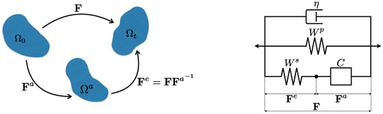
Left: Decomposition of the total deformation gradient tensor F into active F^a and elastic F^e components. Right: Three element model with a viscous dashpot composed of a parallel passive response W^p, a series active response W^s, a contractile element C, and viscous response η.

$$\mathbf{F}={\mathbf{F}}^e{\mathbf{F}}^a.$$ (1)

This multiplicative deformation is analogous to the elastic–plastic decomposition introduced by Lee for plasticity [17]. Note that the active deformation, like plastic deformations, need not be compatible. That is, there need not exist an active deformation mapping for which F^a is a gradient. Nevertheless, we find it helpful to think of the active deformation as describing a local change in the kinematic state of a material point in isolation, producing an intermediate configuration Ω^a, which may be kinematically incompatible with the configurations of neighboring points. Compatibility of the total deformation F to the current configuration Ω_t is restored by the (possibly incompatible) elastic deformation F^e.

2.1. Elastic elements

According to the three-element model (Fig. 2), the response of the parallel element depends on the total deformation, with an elastic response governed by strain energy

$$W^p=W^p(\mathbf{F}).$$ (2)

The serial element, in contrast, should be insensitive to deformations that involve free sliding of inactive cross-bridges. To this effect we define the serial active response according to an energy that depends only on the elastic part of the deformation gradient

$$W^s=W^s({\mathbf{F}}^e)=W^s(\mathbf{F}{\mathbf{F}}^{a-1}).$$ (3)

The total free energy density A is then a sum of the passive and active energies,

$$A=A(\mathbf{F},{\mathbf{F}}^a)=W^p(\mathbf{F})+W^s(\mathbf{F}{\mathbf{F}}^{a-1}).$$ (4)

The equilibrium part of the first Piola–Kirchhoff stress P follows as A_,F(F, F^a).

2.1.1. Passive elasticity

The passive elasticity of the myocardial tissue, represented by the parallel element, has been the subject of extensive study with experiment and modeling. Cardiac muscle has a highly nonlinear, anisotropic elastic response, which is modeled by an elastic energy density function W^p(F). Histology and diffusion tensor MRI have revealed that the microstructure of cardiac tissue is made up of a continuously branching syncytium of cardiomyocytes that are further organized into myolaminar sheetlets [18,19]. This microstructural organization gives rise to a natural definition of a myocardial orthonormal frame (f, s, n) aligned with the principal microstructural axes, where f is aligned with the fibers, s orthogonal to the fibers and in the local sheet plane, and n normal to the sheet. The most general microstructurally informed strain energies [1,20] for the passive response define W^p as a function of orthotropic invariants of the right Cauchy–Green deformation tensor C = F^T F with respect to the myocardial orthonormal frame. Such models are able to fit experimental data from ex vivo myocardial tissue samples placed under shear and biaxial loadings [20]. Earlier biaxial experiments [21,3] were also fit rather well by transversely isotropic models [3,22], of the general form

$$W^p(\mathbf{F})=W^p(I_1,I_2,I_3,I_4),$$ (5)

where

$$I_1=\text{tr}\mathbf{C},I_2=\frac{1}{2}[{(\text{tr}\mathbf{C})}^2-\text{tr}({\mathbf{C}}^2)],I_3=det\mathbf{C}=J^2={(det\mathbf{F})}^2$$ (6)

are the standard isotropic invariants of C, and

$$I_4=\mathbf{C}:[\mathit{f}\otimes \mathit{f}]=\mathit{f}·\mathbf{C}\mathit{f},$$ (7)

is the square of the stretch ratio along the cardiacmyocyte axis, as described by a fiber-directed unit vector f. For the sake of illustration in this paper, we use the energy presented by Lin and Yin [3]

$$\begin{array}{c}{W}^p(\mathbf{F})=C_1(e^Q-1),\\ Q=C_2{(I_1-3)}^2+C_3(I_1-3)(I_4-1)+C_4{(I_4-1)}^2.\end{array}$$ (8)

2.1.2. Active elasticity

Biaxial stretch experiments performed during steady-state contraction have revealed that the elastic response of cardiac tissue is significantly altered during cross-bridge activation [3]. During barium contracture or tetanus, the cross-bridge force generation is steady, such that any change in stress produced by instantaneous strains can be identified with the elastic elements (P + S) in the three-element model.

Lin and Yin [3] found this “active” response to be well modeled by a low-order polynomial strain energy in I₁ and I₄. Consistent with these findings, we define the energy of the serial element as

$$W^s({\mathbf{F}}^e)=D_0+D_1(I_1^e-3)(I_4^e-1)+D_2{(I_1^e-3)}^2+D_3{(I_4^e-1)}^2+D_4(I_1^e-3)+D_5(I_4^e-1),$$ (9)

where $I_1^e$ and $I_4^e$ are the standard invariants of F^e.

2.2. Viscosity

The passive response of biological tissue is not entirely without dissipation. To account for this we may consider additional viscous stresses P^υ, such that

$$\mathbf{P}=A_{,\mathbf{F}}(\mathbf{F},{\mathbf{F}}^a)+{\mathbf{P}}^{\upsilon }(\dot{\mathbf{F}},\mathbf{F}).$$ (10)

Following [14] we consider viscosity laws that derive from a potential, meaning that there exists a function ϕ(Ḟ, F) such that

$${\mathbf{P}}^{\upsilon }={\varphi }_{,\dot{\mathbf{F}}}(\dot{\mathbf{F}},\mathbf{F}).$$ (11)

To be precise, for the sake of illustration we assume Newtonian viscosity and according to [14], the viscous potential is

$$\varphi =\eta \mathit{J}{\mathbf{d}}^{\text{dev}}\cdot {\mathbf{d}}^{\text{dev}},$$ (12)

where η is the viscosity and d^dev is the deviatoric part of the rate of deformation tensor d = sym(ḞF⁻¹). This gives rise to viscous stresses

$${\mathbf{P}}^{\upsilon }=J{\sigma }^{\upsilon }{\mathbf{F}}^{-T},{\sigma }^{\upsilon }=2\eta {\mathbf{d}}^{\text{dev}}.$$ (13)

2.3. Crossbridge kinematics

The kinetics of activation are determined by the contractile element, parameterized kinematically by F^a. Again mirroring the formulation of viscoelasticity by [14] we assume the kinematics of F^a to be restricted by a general “contractile flow rule” of the form

$${\dot{\mathbf{F}}}^a{\mathbf{F}}^{a-1}=\dot{\mathbf{Q}}\mathbf{M},$$ (14)

where Q is an array of internal variables quantifying the local change in sarcomere structure due to cross-bridge sliding, and M an array of tensors that determine the geometric structure of the active deformation. To interpret this flow rule in the context of cardiac mechanics, note that the spatial gradient of a velocity field v = χ _,t (X, t) = χ̇ (X, t) is given by the standard identity [23, e.g.,]

$$\mathbf{L}\equiv {\mathit{v}}_{,\mathit{x}}={(\dot{\mathit{\chi }})}_{,\mathit{X}}{\mathit{X}}_{,\mathit{x}}=\dot{\mathbf{F}}{\mathbf{F}}^{-1}$$ (15)

with F = χ_,X. The left-hand side of (14) can be interpreted as a local velocity gradient of the local (incompatible) active part of the motion, L^a = Ḟ^aF^a−1. Thus we can see the flow rule (14) as reparametrizing the time evolution of the active deformation F^a in terms of internal variable rates Q̇, which represent magnitudes of active velocity gradient.

Example 2.3.1 (One-Dimensional Flow Rule). To put the above relations into the context of microscale physiology, let ℓ(t) denote the current length of a sarcomere (i.e., the distance between adjacent z-lines, as depicted in Fig. 3), and let ℓ₀ be the un-stretched reference length (i.e., prior to diastolic filling). The kinematics of muscle contraction are most commonly described in terms of the “velocity” of contraction for a single sarcomere, υ = ℓ̇. While the (extensive) velocity may be useful in the context of experiments at microscopic scales, or with fixed length samples, a general theory requires description of an intensive measure at each material point. Normalization by current sarcomere length suggests a one-dimensional flow rule for sarcomere length

Fig. 3.

Schematic representation of the sarcomere in its current configuration. The current distance between z-lines is denoted by ℓ and its instantaneous rate of change by ℓ̇.

$$\frac{\dot{\ell }}{\ell }=\dot{Q}.$$ (16)

Defining cardiomyocyte stretch ratio

$$\lambda \equiv \lambda (t)=\frac{\ell }{{\ell }_0},$$ (17)

the total active deformation is

$${\mathbf{F}}^a=\lambda \mathit{f}\otimes \mathit{f}+\mathbf{s}\otimes \mathbf{s}+\mathit{n}\otimes \mathit{n},$$ (18)

with rate

$${\dot{\mathbf{F}}}^a=\dot{\lambda }\mathit{f}\otimes \mathit{f}.$$ (19)

The full tensorial flow rule is then

$${\dot{\mathbf{F}}}^a{\mathbf{F}}^{a-1}=\frac{\dot{\lambda }}{\lambda }\mathit{f}\otimes \mathit{f}=\frac{\dot{\ell }}{\ell }\mathit{f}\otimes \mathit{f}=\dot{\mathit{Q}}\mathit{f}\otimes \mathit{f}.$$ (20)

Example 2.3.2 (Triaxial Flow Rule). Eq. (20) is the simplest example of a contractile flow rule, with arrays Q = {Q} and M = {f⊗f} each containing only a single degree of freedom. More generally, we may model the contraction as involving active motion along a number of geometric modes QM = Σ_iQⁱM_i. While contractile modes M_i could, in general, include extension and shearing of the fiber and sheet structure, at present we consider triaxial contractile flow, i.e., flow in each of the three microstructural directions (fiber, sheet, sheet-normal)

$$\mathbf{Q}={\{Q^f,Q^s,Q^n\}}^T,\mathbf{M}=\{\mathit{f}\otimes \mathit{f},\mathit{s}\otimes \mathit{s},\mathit{n}\otimes \mathit{n}\},$$ (21)

such that flow rule (14) becomes explicitly

$${\dot{\mathbf{F}}}^a{\mathbf{F}}^{a-1}=\dot{\mathbf{Q}}\mathbf{M}={\dot{Q}}_f\mathit{f}\otimes \mathit{f}+{\dot{Q}}_s\mathit{s}\otimes \mathit{s}+{\dot{Q}}_n\mathit{n}\otimes \mathit{n}.$$ (22)

2.4. Cross-bridge kinetics

To model the development of active contractile stresses, we must provide some kinetic equations Defining the evolution of internal variables Q. Assuming these are governed by local thermodynamics, the kinetic equations will be of the general form

$$\dot{\mathbf{Q}}=\mathbf{r}(\mathbf{F},{\mathbf{F}}^a,\mathbf{Q}).$$ (23)

Eq. (23) must model cross-bridge cycling, generally reflecting the relationship between shortening velocity and contractile force, as regulated by biophysical processes in the sarcomere such as Calcium (Ca²⁺) binding and tropomyosin kinetics. Calcium concentration is, in turn, controlled by the electrophysiological response of the cell [24,25], which is modeled locally by first order rate equations similar in form to (23). Thus, it would be possible to expand the internal variable array Q to include electrophysiological variables, pointing the way toward a fully coupled electromechanical formulation. For now we assume the right-hand side of (23) to have time varying coefficients that are determined by the electrophysiology.

The next step is to design a rate function r in (23) that models the evolution of shortening and contractile force in the sarcomere. While detailed models of cross-bridge kinetics are available [26,6] here we are particularly interested in developing a model that retains a variational structure. Toward this goal, as in [14], we define the thermodynamic force conjugate to F^a as

$$\mathbf{T}=-A_{,{\mathbf{F}}^a}.$$ (24)

Taking the time derivative of A while holding F fixed, we obtain

$$\dot{A}{|}_{\mathit{F}}=A_{,{\mathbf{F}}^{\mathbf{a}}}{\dot{\mathbf{F}}}^a+A_{,\mathbf{Q}}\dot{\mathbf{Q}}$$ (25a)

$$=-\mathbf{T}\dot{\mathbf{Q}}\mathbf{M}{\mathbf{F}}^a+A_{,\mathbf{Q}}\dot{\mathbf{Q}}$$ (25b)

$$=(-\mathbf{T}\cdot (\mathbf{M}{\mathbf{F}}^a)+A_{,\mathbf{Q}})\dot{\mathbf{Q}},$$ (25C)

where we used the flow rule Eq. (14) in Eq. (25b). Writing Ȧ = −YQ̇, from Eq. (25c) the thermodynamic force conjugate to the internal variables Q is

$$\mathbf{Y}=\mathbf{T}\cdot (\mathbf{M}{\mathbf{F}}^a)-A_{,\mathbf{Q}}.$$ (26)

We consider kinetic equations that derive from a potential ψ(Y), i.e.,

$$\dot{\mathbf{Q}}={\psi }_{,\mathbf{Y}}(\mathbf{Y}).$$ (27)

Given a function ψ we may alternatively treat Q̇ as the independent variable, and perform a Legendre transformation, to obtain a dual potential

$${\psi }^{\ast }(\dot{\mathbf{Q}})=\underset{\mathbf{Y}}{sup}[\mathbf{Y}\cdot \dot{\mathbf{Q}}-\psi (\mathbf{Y})],$$ (28)

such that

$${\psi }_{,\dot{\mathbf{Q}}}^{\ast }(\dot{\mathbf{Q}})=\mathbf{Y}.$$ (29)

Example 2.4.1 (One-Dimensional Contraction). We may relate these new variables back to the 1-D context of Example 2.3.1. In general, the energy density of the three-element model (4) has no explicit dependence on Q, so A_,Q = 0, and

$$\mathbf{Y}=\mathbf{T}\cdot (\mathbf{M}){\mathbf{F}}^a=\mathbf{M}\cdot (\mathbf{T}{\mathbf{F}}^{aT}).$$ (30)

Furthermore, differentiation of (4) gives

$$\mathbf{P}=A_{,\mathbf{F}}={\mathbf{P}}^p+{\mathbf{P}}^s;$$ (31)

$$\mathbf{T}=-A_{,{\mathbf{F}}^a}={\mathbf{F}}^{eT}{\mathbf{P}}^s,$$ (32)

where

$${\mathbf{P}}^p=W_{,\mathbf{F}}^p\text{and}{\mathbf{P}}^s=W_{,{\mathbf{F}}^e}^s{\mathbf{F}}^{a-T}$$ (33)

are the first Piola–Kirchhoff stresses of the parallel passive and serial active elements. Also

$$\mathbf{Y}=\mathbf{M}\cdot ({\mathbf{F}}^{eT}{\mathbf{P}}^s{\mathbf{F}}^{aT}).$$ (34)

For a purely one-dimensional contraction (cf. Example 2.3.1) with Q = {Q^f} and M = {f⊗f}, this simplifies to

$$Y^f=\mathit{f}\cdot ({\mathbf{F}}^{eT}{\mathbf{P}}^s{\mathbf{F}}^{aT})\mathit{f},$$ (35)

which we can identify as an equivalent uniaxial contractile stress.

Q̇^f represents the rate of contractile shortening such that Eq. (29) simplifies to

$$Y^f=\frac{d\psi \ast }{d\dot{Q}f}$$ (36)

specifying an effective force–velocity relation for the sarcomere.

Example 2.4.2 (Hill's Force–Velocity Curve). To model ψ* we return to the work of A.V. Hill [12,16], which proposes the phenomenological hyperbolic force–velocity relation for a single sarcomere in tetanic contraction

$$(\upsilon +b)(F+a)=b(F_0+a),$$ (37)

where F is the tension, υ is the shortening velocity, and F₀, a, and b are constants. Defining ϕ^F ≡ a/F₀ and ϕ^υ ≡ b/υ₀, we can write Eq. (37) more conveniently as

$$F(\upsilon )=F_0({\varphi }^{\upsilon }\frac{{\varphi }^F+1}{{\varphi }^{\upsilon }+\frac{\upsilon }{{\upsilon }_0}}-{\varphi }^F).$$ (38)

Identifying Y^f with F and Q̇^f with −υ we find dψ* = Y^fdQ̇^f = −Fdυ, which we can integrate to obtain, within an arbitrary constant,

$${\psi }^{\ast }({\dot{Q}}^f)=-F_0{\upsilon }_0[\frac{{\varphi }^F{\dot{Q}}^f}{{\upsilon }_0}+{\varphi }^{\upsilon }(1+{\varphi }^F)ln({\varphi }^{\upsilon }-\frac{{\dot{Q}}^f}{{\upsilon }_0}\left)\right].$$ (39)

From the plot of (38) in Fig. 5(a) we can see that F₀ is the isometric force (where Q̇^f = 0), and υ₀ represents the maximum or unloaded shortening velocity (Q̇^f → −υ₀ as Y^f → 0).

Fig. 5.

Left: the calcium transient from the Mahajan et al. [25] cell model is used to modulate the peak force in the fiber. Right: the force–velocity relationship from Eq. (41) is plotted for various values of F₀(t).

However, the kinetic potential Eq. (39) derived from Hill's force–velocity relation presents a singularity as Q̇^f → ϕ^υυ₀, i.e., during retrograde motion or lengthening of the contractile element C. In practice, care must be taken to avoid this singularity either by a judicious choice of time steps or by an alternative definition of ψ*.

For our study, we propose a new version of ψ*, which does not have such a singularity but also preserves the hyperbolic force–velocity relationship of (38)

$${\psi }^{\ast }({\dot{Q}}^f)=\frac{F_0{\upsilon }_0}{\beta }exp\left[\beta \frac{{\dot{Q}}^f}{{\upsilon }_0}\right],$$ (40)

where β is a non-dimensional parameter that controls the shape of the force–velocity response. By differentiating Eq. (40) with respect to Q̇^f, we compute the force along the cardiomyocyte direction as

$$Y^f=F_{0}exp\left[\beta \frac{{\dot{Q}}^f}{{\upsilon }_0}\right].$$ (41)

For the purpose of comparison, we plot the force–velocity relationship and the kinetic potential using both Hill's equation and our modified Hill's equation in Fig. 4.

Fig. 4.

Left: force versus velocity relationship obtained using Hill's equation and our modified Hill's equation to avoid the singularity shown in Eq. (39). Right: the force–velocity relationships are integrated to produce the kinetic potentials from Hill's equation and our modified equation. For Hill's equation, the parameters chosen are F₀ = 25 m N, ${\upsilon }_0=3.0\frac{\text{length}}{\mathrm{s}}$, a = 4.4 m N, and $b=0.59\frac{\text{length}}{\mathrm{s}}$ as described in [27]. For our exponential function F₀ = 25 m N, ${\upsilon }_0=3.0\frac{\text{length}}{\mathrm{s}}$, and β = 4.0.

The contraction of sarcomeres is driven by electrophysiological changes within the cell. During myocardial electrical activation, calcium is released into the cell membrane space, allowing for actin–myosin binding and the initiation of crossbridge cycling. Therefore, in our current formulation, we scale F₀(t), and consequently the force–velocity curve, with the calcium transient. Here we use the Mahajan et al. [25] cell model to compute intracellular calcium during a cardiac cycle (Fig. 5).

3. Variational constitutive updates

As discussed in [14], a potential function D can be formulated to yield the above constitutive equations in a variational manner:

$$D(\dot{\mathbf{F}},\dot{\mathbf{Q}})=A_{,\mathbf{F}}\cdot \dot{\mathbf{F}}-\mathbf{Y}\cdot \dot{\mathbf{Q}}+{\psi }^{\ast }(\dot{\mathbf{Q}})+\varphi (\dot{\mathbf{F}}).$$ (42)

Optimizing D with respect to Q̇ returns the kinetic relations and further yields D^eff(Ḟ) which acts as a rate-potential for the first Piola–Kirchhoff stress tensor

$$\mathbf{P}=D_{,\dot{\mathbf{F}}}^{\text{eff}}=A_{,\mathbf{F}}+{\varphi }_{,\dot{\mathbf{F}}}.$$ (43)

In solving the above problem, we concern ourselves with a time increment from t_k to t_k+1 where a material point evolves from its current state (F_k, ${\mathbf{F}}_k^a$, Q_k) to a new state (F_k+1, ${\mathbf{F}}_{k+1}^a$, Q_k+1). Following [14], we integrate the flow rule (Eq. (14)) to yield an update for F^a

$${\mathbf{F}}_{k+1}^a=exp[\Delta \mathbf{Q}\mathbf{M}]{\mathbf{F}}_k^a,$$ (44)

where ΔQ = Q_k+1 − Q_k.

Example 3.0.1 (Flow Rule Updates for 3D Sarcomere Mechanics). Since {f s n} and {ΔQ^f ΔQ^s ΔQⁿ} are, respectively, the eigenvectors and eigenvalues of ΔQM, the flow rule update is

$${\mathbf{F}}_{k+1}^a=exp(\Delta Q^f\mathit{f}\otimes \mathit{f}+\Delta Q^s\mathit{s}\otimes \mathit{s}+\Delta Q^n\mathit{n}\otimes \mathit{n}){\mathbf{F}}_k^a$$ (45)

$$=[e^{\Delta Q^f}\mathit{f}\otimes \mathit{f}+e^{\Delta Q^s}\mathit{s}\otimes \mathit{s}+e^{\Delta Q^n}\mathit{n}\otimes \mathit{n}]{\mathbf{F}}_k^a.$$ (46)

Following [14] and using the viscous (Eq. (12)) and kinetic (Eq. (40)) potentials, we can define the incremental energy density function as

$$W({\mathbf{F}}_{k+1};{\mathbf{F}}_k,{\mathbf{Q}}_k)=\Delta t\varphi (\frac{{\mathbf{F}}_{k+1}-{\mathbf{F}}_k}{\Delta t};{\mathbf{F}}_{k+\alpha })+\underset{{\mathbf{Q}}_{k+1}}{min}\{A({\mathbf{F}}_{k+1},{\mathbf{F}}_{k+1}^a,{\mathbf{Q}}_{k+1})-A({\mathbf{F}}_k,{\mathbf{F}}_k^a,{\mathbf{Q}}_k)+\Delta t{\psi }^{\ast }(\frac{{\mathbf{Q}}_{k+1}-{\mathbf{Q}}_k}{\Delta t},Q_{k+\alpha }\left)\right\},$$ (47)

where the parameter α controls the state at which the viscous and kinetic potentials are evaluated, i.e.,

$${\mathbf{F}}_{k+\alpha }=(1-\alpha ){\mathbf{F}}_k+\alpha {\mathbf{F}}_{k+1};$$ (48)

$${\mathbf{Q}}_{k+\alpha }=(1-\alpha ){\mathbf{Q}}_k+\alpha {\mathbf{Q}}_{k+1}.$$ (49)

Taking the first variation of W with respect to F and using the stationarity condition for Q_k+1, we write the first Piola–Kirchhoff stress tensor as

$${\mathbf{P}}_{k+1}=\frac{\partial W}{\partial {\mathbf{F}}_{k+1}}=A_{,\mathbf{F}}({\mathbf{F}}_{k+1},{\mathbf{F}}_{k+1}^a,{\mathbf{Q}}_{k+1})+{\mathbf{P}}^{\upsilon }(\frac{{\mathbf{F}}_{k+1}-{\mathbf{F}}_k}{\Delta t};{\mathbf{F}}_{k+\alpha }).$$ (50)

The tangent moduli are found by linearizing P_k+1 with respect to F_k+1

$$\mathbf{C}=\frac{\partial {\mathbf{P}}_{k+1}}{\partial {\mathbf{F}}_{k+1}}=W_{,{\mathbf{F}}_{k+1}{\mathbf{F}}_{k+1}}+W_{,{\mathbf{F}}_{k+1},{\mathbf{Q}}_{k+1}}\frac{\partial {\mathbf{Q}}_{k+1}}{\partial {\mathbf{F}}_{k+1}}.$$ (51)

Using the stationarity condition of W with respect to Q_k+1

$$W_{{\mathbf{Q}}_{k+1},{\mathbf{F}}_{k+1}}+W_{{\mathbf{Q}}_{k+1},{\mathbf{Q}}_{k+1}}\frac{\partial {\mathbf{Q}}_{k+1}}{\partial {\mathbf{F}}_{k+1}}=0,$$ (52)

we can rewrite Eq. (51) as

$$\mathbf{C}=W_{,{\mathbf{F}}_{k+1}{\mathbf{F}}_{k+1}}-W_{,{\mathbf{F}}_{k+1}{\mathbf{Q}}_{k+1}}{W}_{,{\mathbf{Q}}_{k+1}{\mathbf{Q}}_{k+1}}^{-1}{W}_{,{\mathbf{Q}}_{k+1}{\mathbf{F}}_{k+1}}.$$ (53)

4. Numerical examples

In the numerical examples discussed below, we use energy laws published in the literature and modify them such that the material response they describe is nearly incompressible. To this effect, we penalize the volumetric deformation by adding two terms whose coefficients are marked with * to the energy laws, as seen in Eqs. (54) and (55). Additionally, we remove the terms in the energy laws that produce a non-zero stress free reference state. For the parallel (passive) element, we use a modified version of the Humphrey [22,28] energy law:

$$W^p(\mathbf{F})=C_1{(\sqrt{I_4}-1)}^2+C_2{(\sqrt{I_4}-1)}^3+C_3(I_1-3)(\sqrt{I_4}-1)+C_4{(I_1-3)}^2+C_5^{\ast }(I_1-3-2lnJ)+\frac{C_6^{\ast }}{2}{(lnJ)}^2.$$ (54)

For the serial (active) element, we use the following strain energy law (modified from Lin and Yin [3]):

$$W^s({\mathbf{F}}^e)=D_1(I_1^e-3)(I_4^e-1)+D_2{(I_1^e-3)}^2+D_3{(I_4^e-1)}^2+D_4^{\ast }(I_1^e-3-2ln{J}^e)+\frac{D_5^{\ast }}{2}{(ln{J}^e)}^2.$$ (55)

In the following numerical examples, the values for the Newtonian viscosity and the sarcomere force/shortening velocity curves were varied to yield a physiologic contraction. A summary of the parameter values is provided in Table 1.

Table 1.

Parameter values for numerical examples.

Passive parameters (C1–C4 taken from Humphrey [22])	C1 = 15.98 g/cm2
	C2 = 55.85 g/cm2
	C3 = 3.590 g/cm2
	C4 = 30.21 g/cm2
	$C_5^{\ast }=3.590\mathrm{g}/{\text{cm}}^2$
	$C_6^{\ast }=64.62\mathrm{g}/{\text{cm}}^2$
Active parameters (C1–C3 taken from Lin and Yin [3])	D1 = −38.70 g/cm2
	D2 = 40.83 g/cm2
	D3 = 25.12 g/cm2
	$D_4^{\ast }=9.51\mathrm{g}/{\text{cm}}^2$
	$D_5^{\ast }=171.18\mathrm{g}/{\text{cm}}^2$
Kinetic potential parameters (υ0 taken from Edman and Nilsson [27])	F0 = 50.0 − 100.0 m N
	β = 4.0
	υ0 = 3.0/s
Newtonian viscous potential parameters	η = 0.0, 0.1, 1.0, 10.0 g s/cm2

4.1. Material point

Using the presented variational approach, we first test two classes of simulations, characteristic of muscle experiments from literature, at a single material point. In the first type of experiments, a section of muscle tissue is pre-stretched from its resting state and then released to allow free contraction. To reproduce these experiments in our simulations, we start by imposing the following purely uniaxial deformation gradient:

$$\mathbf{F}=\left[\begin{array}{ccc}1.2& 0& 0\\ 0& 1.0& 0\\ 0& 0& 1.0\end{array}\right].$$ (56)

During this phase, force Y^f in the contractile element is zero and thus the element slides freely without a resisting force, i.e. F = F^a. Consequently, the stress generated in the three element model results only from the parallel passive element. Next, the length constraint is released and the model is allowed to return to its relaxed state while the peak isometric force F₀(t) in the kinetic potential is increased. In order to study the effect of viscosity in these experiments, we vary the viscous parameter η and set it to one of the following values: 0 (no viscosity), 0.1 (low viscosity), 1.0 (medium viscosity), and 10.0 (high viscosity). In Fig. 6 (left), we see that viscosity plays a large role in the contraction/relaxation of the model. When there is no viscosity in the system, the reference length changes by approximately 12%. In contrast, at high viscosity, the effect of contraction is overshadowed by the slow relaxation. During relaxation starting from the release of the length constraint, the elastic stresses, the sum of the stresses in the parallel and serial elements, decay to zero. As seen in Fig. 6 (right), the rate of relaxation decreases as the viscosity increases. Having the ability to tune the viscous parameter is important for modeling lusitropy (i.e., the rate of relaxation following contraction) that, for example, is decreased in several forms of heart failure.

Fig. 6.

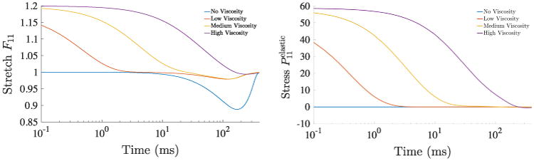
In the first class of material point experiments, a 20% stretch is imposed in the fiber direction and then released. Isometric force modulation F₀(t) also begins at time 0 ms. (Left) Stretch versus time plotted for various viscous parameters, 0 (no viscosity), 0.1 (low viscosity), 1.0 (medium viscosity), and 10.0 (high viscosity). Note that in the case of high viscosity, the slow relaxation overshadows the effect of contraction. (Right) Elastic stress in the model plotted against time for the same viscous parameters.

In the second class of experiments we simulate a section of cardiac muscle tissue that is held at a constant length (F = I) and contraction is then initiated. In this case, as F₀(t) increases, the contractile element shortens, i.e., Q^f decreases, and the tensile force Y^f increases. Through the flow rule (Eq. (14)), the component of the active deformation gradient in the fiber direction also decreases (Fig. 7 (left)). As a result, a time-varying stress is generated in the serial active element (Fig. 7 (right)). However, since the model length is held fixed, the stress in the parallel passive element is zero.

Fig. 7.

In the second class of material point experiments, the model undergoes contraction while its length is held fixed (F = I). The internal variable Q^f and the component of the active deformation gradient F^a in the fiber direction decrease (left) while tensile stresses increase in the series (active) element (right).

4.2. Strip of myocardial tissue

In this numerical example, we simulate the contraction of a rectangular cuboid representative of a strip of myocardial tissue oriented transmurally across the left ventricle wall. The rectangular cuboid has dimensions 1 cm × 0.20 cm × 0.20 cm and is meshed with 1920 linear tetrahedral elements with an approximate edge length of 0.05 cm (Fig. 8). As a boundary condition, a spring foundation was imposed on the yz-plane and additional roller supports were added to remove the rigid body rotation about the x-axis.

Fig. 8.

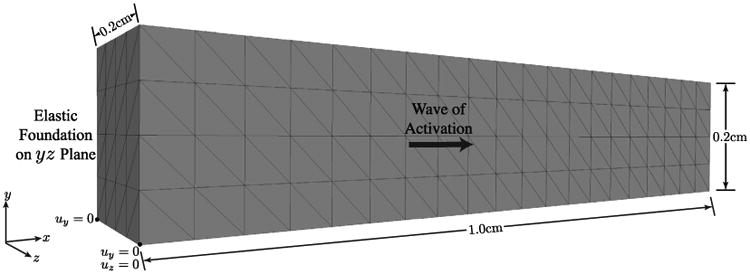
Rectangular cuboid representative of a strip of tissue across the ventricular wall: simulation setup and geometry.

As previously discussed, the contraction at each location is controlled using isometric force F₀(t) in the kinetic potential ψ*. In order to simulate a wave of activation/contraction along the long-axis of the cuboid (x-axis), we impose a 60 cm/s conduction velocity. In this experimental setup, we examine two different fiber distributions:

1. Fibers all aligned along the x-axis (Fig. 9 (left)).

2. Fibers perpendicular to the long axis and rotated about this axis from −60° (epicardium) to +60° (endocardium) (Fig. 9 (right)), which is representative of a transmural block of myocardium.

Fig. 9.

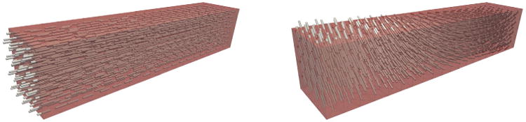
Fiber distributions used in the simulation of contraction in a strip of cardiac tissue: (left) fibers aligned along the long-axis and (right) fibers perpendicular to the long axis and rotated from −60° (epicardium) to +60° (endocardium).

In the first stage of the simulation, a wave of activation travels from the left to the right of the rectangular domain and initiates contraction as seen by the distribution of Q^f along the long axis in Fig. 10. The fiber strain Q^f peaks at approximately 200 ms, which corresponds to the maximum of the calcium transient and consequently, to the maximum isometric force F₀(t). Subsequently, following the decay of the calcium transient (corresponding to the reuptake of calcium by the sarcoplasmic reticulum) the tissue undergoes relaxation, which completes at approximately 400 ms.

Fig. 10.

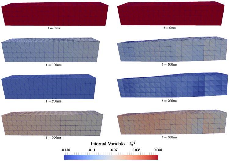
Contraction simulation of a strip of cardiac tissue. A left to right wave of activation initiates contraction as shown by distribution of the internal variable Q^f . The fiber strain peaks at approximately 200 ms and relaxes by about 400 ms. Left: the simulation with fibers aligned along the long-axis shows wall compression and no twisting. Right: the simulation with fibers perpendicular to the long-axis and varying across the wall shows wall thickening and twisting as expected for in vivo myocardium.

The mechanisms of deformation of the models with the two different fiber distributions show key differences. If the fibers all point along the long-axis, the tissue compresses across the wall with no torsion. In contrast, with rotating fibers about the long-axis, we obtain tissue thickening and twisting across the wall. Reproducing thickening and twisting is important since both features are observed clinically during contraction.

4.3. Ventricular geometry

In our final numerical example, we simulate a contractile event in an ellipsoidal geometry representative of the left ventricle of a human heart. The ellipsoidal geometry was meshed with 16 583 linear tetrahedral elements (Fig. 11 (left)). Rule-based fibers were computed at the barycenters of each tetrahedral element such that their orientation varies linearly from −53.5° (epicardium) to 39.5° (endocardium) in accordance with [29] (Fig. 11 (right)).

Fig. 11.

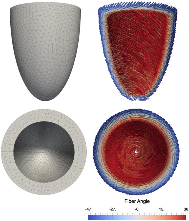
Ellipsoidal geometry representative of the human heart left ventricle. (Left) Mesh composed of 16583 tetrahedral elements. (Right) Rule-based fibers linearly varying from −53.5° (epicardium) to 39.5° (endocardium) about the axis perpendicular to the ellipsoid mid-surface [29].

In order to simulate the electromechanical coupling, we first solve the monodomain equation of electrophysiology [30] using the Mahajan et al. [25] cell model. To begin the activation sequence, we apply a stimulus current to 145 nodes at the apex of the ventricle and then measure the time required to reach 0 mV in every element in the model (Fig. 12). This activation time is used to begin the modulation of F₀(t) at each element and initiate contraction.

Fig. 12.

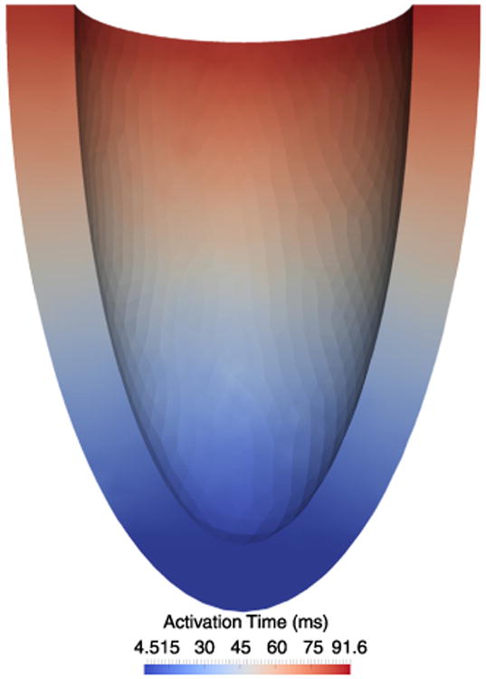
Wave of activation computed by applying a stimulus current to the apex of the ellipsoidal geometry and solving the monodomain equation of cardiac electrophysiology. The time required for each element to reach 0 mV is shown. These activation times are used to initiate contraction, i.e., to determine the beginning of the isometric force modulation.

As boundary conditions in the mechanics problem, we apply an elastic spring foundation to the epicardial wall of the left ventricle to simulate the pericardium. That is, a spring force is applied to every node on the surface in the normal direction computed by averaging the normals of the surface elements to which the node is connected. During contraction we note (Fig. 13): (i) wall thickening, (ii) a twist angle of 20°, and (iii) reduction of the cavity volume corresponding to an ejection fraction of 49%. These findings are consistent with clinically observed phenomena. We also notice that the myocardial volume decreases by approximately 10% at maximum contraction. This result deviates from the literature according to which the myocardium is incompressible or nearly incompressible [31,32].

Fig. 13.

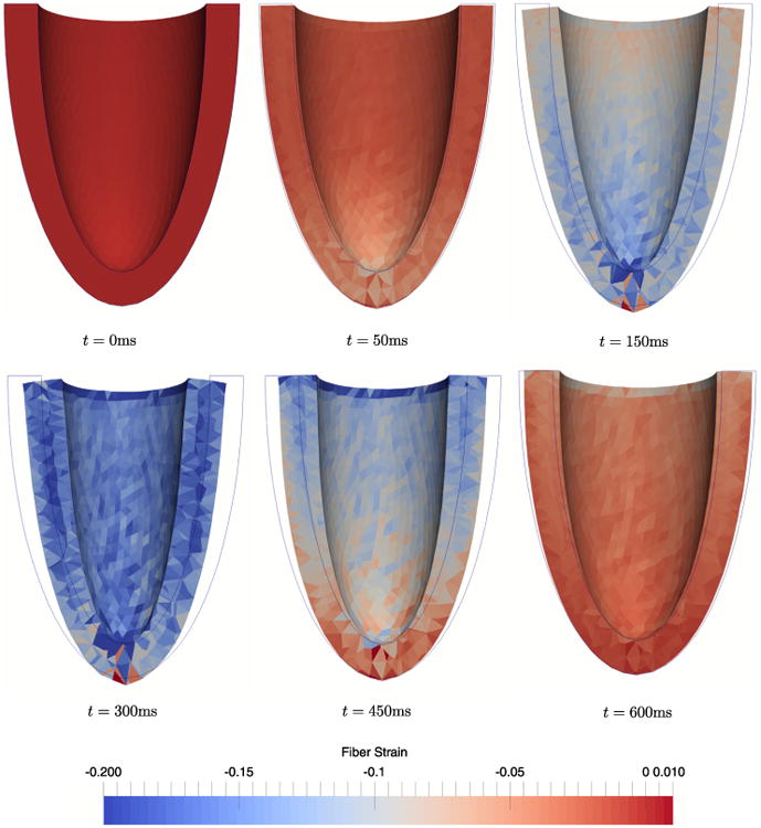
Snapshots during contraction of an ellipsoidal geometry. We observe wall thickening, base-to-apex twisting, and reduction of the cavity volume, which corresponds to a maximum ejection fraction of 49%.

5. Conclusion

In this work, we use the variational formulation for a viscoplastic constitutive model [14] as the basis for modeling electrically active soft tissue where the internal variables are the sarcomere stretches. We have also shown how this model can be coupled to the electrophysiology through the kinetic potential. In future research, we aim to refine the model and validate it with experimental evidence. The first step consists in improving the constitutive models that describe the active (W^s) and passive (W^p) responses of the myocardium, e.g., by enforcing the tissue incompressibility constraint. Further, it is crucial for this modeling framework to identify the correct kinetic potentials that describe active force generation and sarcomere shortening velocities. In this work, we have used a Hill-type force–velocity relation and modulated peak force with respect to the calcium transient. A more involved set of relations will consider other parameters such as actin–myosin binding kinetics, sarcomere length, etc. Finally, our goal is to apply this model to an anatomically accurate ventricular geometry and microstructure (i.e., fiber orientations) and to study the effect of more realistic boundary conditions.

Highlights.

• Unifying constitutive modeling framework to simulate cardiac contraction.

• Hill-like three element model together with a viscous dashpot.

• Single variational principle for stress–strain relations and kinetic rate equations.

• Hill's force–velocity relationship as the basis for the kinetic equations.

• Simulated contraction of a representative left ventricle geometry using FEM.

References

- 1.Usyk T, Mazhari R, McCulloch A. Effect of laminar orthotropic myofiber architecture on regional stress and strain in the canine left ventricle. J Elast Phys Sci Solids. 2000;61(1–3):143–164. [Google Scholar]
- 2.Nash MP, Panflov AV. Electromechanical model of excitable tissue to study reentrant cardiac arrhythmias. Prog Biophys Mol Biol. 2004;85(2):501–522. doi: 10.1016/j.pbiomolbio.2004.01.016. [DOI] [PubMed] [Google Scholar]
- 3.Lin D, Yin F. A multiaxial constitutive law for mammalian left ventricular myocardium in steady-state barium contracture or tetanus. J Biomech Eng. 1998;120(4):504–517. doi: 10.1115/1.2798021. [DOI] [PubMed] [Google Scholar]
- 4.Pathmanathan P, Chapman S, Gavaghan D, Whiteley J. Cardiac electromechanics: the effect of contraction model on the mathematical problem and accuracy of the numerical scheme. Quart J Mech Appl Math. 2010:hbq014. [Google Scholar]
- 5.Göktepe S, Kuhl E. Electromechanics of the heart: a unified approach to the strongly coupled excitation–contraction problem. Comput Mech. 2010;45(2–3):227–243. [Google Scholar]
- 6.Guccione J, Waldman L, McCulloch A. Mechanics of active contraction in cardiac muscle: Part ii - Cylindrical models of the systolic left ventricle. J Biomech Eng. 1993;115(1):82–90. doi: 10.1115/1.2895474. [DOI] [PubMed] [Google Scholar]
- 7.Nardinocchi P, Teresi L. On the active response of soft living tissues. J Elasticity. 2007;88(1):27–39. [Google Scholar]
- 8.Cherubini C, Filippi S, Nardinocchi P, Teresi L. An electromechanical model of cardiac tissue: Constitutive issues and electrophysiological effects, Progress in biophysics and molecular biology. 2008;97(2):562–573. doi: 10.1016/j.pbiomolbio.2008.02.001. [DOI] [PubMed] [Google Scholar]
- 9.Ambrosi D, Arioli G, Nobile F, Quarteroni A. Electromechanical coupling in cardiac dynamics: the active strain approach. SIAM J Appl Math. 2011;71(2):605–621. [Google Scholar]
- 10.Pezzuto S, Ambrosi D. Active contraction of the cardiac ventricle and distortion of the microstructural architecture. Int J Numer Methods Biomed Eng. 2014;30(12):1578–1596. doi: 10.1002/cnm.2690. [DOI] [PubMed] [Google Scholar]
- 11.Pezzuto S, Ambrosi D, Quarteroni A. An orthotropic active–strain model for the myocardium mechanics and its numerical approximation. Eur J Mech A Solids. 2014;48:83–96. [Google Scholar]
- 12.Hill A. The heat of shortening and the dynamic constants of muscle. Proc R Soc Lond Biol. 1938;126(843):136–195. [Google Scholar]
- 13.Göktepe S, Menzel A, Kuhl E. The generalized hill model: A kinematic approach towards active muscle contraction. J Mech Phys Solids. 2014;72:20–39. doi: 10.1016/j.jmps.2014.07.015. [DOI] [PMC free article] [PubMed] [Google Scholar]
- 14.Ortiz M, Stainier L. The variational formulation of viscoplastic constitutive updates. Comput Methods Appl Mech Engrg. 1999;171(3):419–444. [Google Scholar]
- 15.Gizzi A, Pandolf A. Visco-hyperelasticity of electro-active soft tissues. Procedia IUTAM. 2015;12:162–175. [Google Scholar]
- 16.Fung YC. Biomechanics: Mechanical Properties of Living Tissues. Springer Science & Business Media. 2013 [Google Scholar]
- 17.Lee EH. Elastic–plastic deformation at finite strains. J Appl Mech. 1969;36(1):1–6. [Google Scholar]
- 18.LeGrice IJ, Smaill B, Chai L, Edgar S, Gavin J, Hunter PJ. Laminar structure of the heart: ventricular myocyte arrangement and connective tissue architecture in the dog. Am J Physiol- Heart Circ Physiol. 1995;269(2):H571–H582. doi: 10.1152/ajpheart.1995.269.2.H571. [DOI] [PubMed] [Google Scholar]
- 19.Kung GL, Nguyen TC, Itoh A, Skare S, Ingels NB, Miller DC, Ennis DB. The presence of two local myocardial sheet populations confirmed by diffusion tensor mri and histological validation. J Magn Reson Imaging. 2011;34(5):1080–1091. doi: 10.1002/jmri.22725. [DOI] [PMC free article] [PubMed] [Google Scholar]
- 20.Holzapfel GA, Ogden RW. Constitutive modelling of passive myocardium: a structurally based framework for material characterization. Phil Trans R Soc A. 2009;367(1902):3445–3475. doi: 10.1098/rsta.2009.0091. [DOI] [PubMed] [Google Scholar]
- 21.Demer LL, Yin F. Passive biaxial mechanical properties of isolated canine myocardium. J Physiol. 1983;339:615. doi: 10.1113/jphysiol.1983.sp014738. [DOI] [PMC free article] [PubMed] [Google Scholar]
- 22.Humphrey J, Strumpf R, Yin F. Determination of a constitutive relation for passive myocardium: I. A new functional form. J Biomech Eng. 1990;112(3):333–339. doi: 10.1115/1.2891193. [DOI] [PubMed] [Google Scholar]
- 23.Holzapfel GA. Nonlinear solid mechanics: a continuum approach for engineering science. Meccanica. 2002;37(4):489–490. [Google Scholar]
- 24.Bers DM. Calcium cycling and signaling in cardiac myocytes. Annu Rev Physiol. 2008;70:23–49. doi: 10.1146/annurev.physiol.70.113006.100455. [DOI] [PubMed] [Google Scholar]
- 25.Mahajan A, Shiferaw Y, Sato D, Baher A, Olcese R, Xie LH, Yang MJ, Chen PS, Restrepo JG, Karma A, et al. A rabbit ventricular action potential model replicating cardiac dynamics at rapid heart rates. Biophys J. 2008;94(2):392–410. doi: 10.1529/biophysj.106.98160. [DOI] [PMC free article] [PubMed] [Google Scholar]
- 26.Hunter P, Mc Culloch A, Ter Keurs H. Modelling the mechanical properties of cardiac muscle. Prog Biophys Mol Biol. 1998;69(2):289–331. doi: 10.1016/s0079-6107(98)00013-3. [DOI] [PubMed] [Google Scholar]
- 27.Edman K, Nilsson E. The mechanical parameters of myocardial contraction studied zit a constant length of the contractile element. Acta Physiol Scand. 1968;72(1–2):205–219. doi: 10.1111/j.1748-1716.1968.tb03843.x. [DOI] [PubMed] [Google Scholar]
- 28.Humphrey J, Strumpf R, Yin F. Determination of a constitutive relation for passive myocardium: ii -Parameter estimation. J Biomech Eng. 1990;112(3):340–346. doi: 10.1115/1.2891194. [DOI] [PubMed] [Google Scholar]
- 29.Ennis DB, Nguyen TC, Riboh JC, Wigströ L, Harrington KB, Daughters GT, Ingels NB, Miller DC. Myofiber angle distributions in the ovine left ventricle do not conform to computationally optimized predictions. J Biomech. 2008;41(15):3219–3224. doi: 10.1016/j.jbiomech.2008.08. [DOI] [PMC free article] [PubMed] [Google Scholar]
- 30.Krishnamoorthi S, Perotti LE, Borgstrom NP, Ajijola OA, Frid A, Ponnaluri AV, Weiss JN, Qu Z, Klug WS, Ennis DB, et al. Simulation methods and validation criteria for modeling cardiac ventricular electrophysiology. PLoS One. 2014;9(12):e114494. doi: 10.1371/journal.pone.0114494. [DOI] [PMC free article] [PubMed] [Google Scholar]
- 31.Yin F, Chan C, Judd RM. Compressibility of perfused passive myocardium. Am J Physiol- Heart Circ Physiol. 1996;271(5):H1864–H1870. doi: 10.1152/ajpheart.1996.271.5.H1864. [DOI] [PubMed] [Google Scholar]
- 32.Rodriguez I, Ennis DB, Wen H. Noninvasive measurement of myocardial tissue volume change during systolic contraction and diastolic relaxation in the canine left ventricle. Magn Reson Med. 2006;55(3):484–490. doi: 10.1002/mrm.20786. [DOI] [PMC free article] [PubMed] [Google Scholar]