Model Predictive Filtering for Improved Temporal Resolution in MRI Temperature Imaging

Abstract

A novel method for reconstructing MRI temperature maps from undersampled data is presented. The method, model predictive filtering, combines temperature predictions from a preidentified thermal model with undersampled k-space data to create temperature maps in near real time. The model predictive filtering algorithm was implemented in three ways: using retrospectively undersampled k-space data from a fully sampled two-dimensional gradient echo (GRE) sequence (reduction factors R = 2.7 to R = 7.1), using actually undersampled data from a two-dimensional GRE sequence (R = 4.8), and using actually undersampled data from a three-dimensional GRE sequence (R = 12.1). Thirty-nine high-intensity focused ultrasound heating experiments were performed under MRI monitoring to test the model predictive filtering technique against the current gold standard for MR temperature mapping, the proton resonance frequency shift method. For both of the two-dimensional implementations, the average error over the five hottest voxels from the hottest time frame remained between ±0.8°C and the temperature root mean square error over a 24 × 7 × 3 × 25-voxel region of interest remained below 0.35°C. The largest errors for the three-dimensional implementation were slightly worse: −1.4°C for the mean error of the five hottest voxels and 0.61°C for the temperature root mean square error. Magn Reson Med 63:1269–1279, 2010.

Thermal therapies are increasingly being seen as a viable method for noninvasive treatment of tumor cells (1–6). During a typical MR-guided high-intensity focused ultrasound (HIFU) procedure, ultrasound is used to noninvasively heat a small volume within the tumor to the point of cell death while sparing surrounding normal tissues (7,8). The tumor is fully ablated by treating multiple small subvolumes successively through the tumor in a continuous scanning pattern or with a cooling period in between sonications (2,3). MRI can detect irreversible damage in soft tissue due to heating and measure temperature changes in a variety of tissue types (9–11). Real time monitoring by MRI to control heating ensures tumor treatment efficacy while sparing surrounding normal tissues. Of the several MRI methods that are documented to measure temperature, the proton resonance frequency (PRF) shift method is by far the most popular (12,13). While many investigators have performed successful MR-guided HIFU procedures with standard PRF thermometry, improved spatial and temporal resolution would provide the clinician with more detailed temperature data, potentially reducing treatment times while ensuring the achievement of safety and efficacy.

MR thermometry requires high spatial resolution to accommodate the small, nonuniform shape of the ultrasound focal zone and nonuniform tissue boundaries. A typical HIFU focal zone is elongated in the direction of beam propagation, with full width at half maximum dimensions of 13 mm × 2 mm. The power deposition over this volume is approximately gaussian shaped, and therefore imaging with voxels larger than 1–2 mm³ isotropic leads to temperature averaging effects that induce errors in the temperature measurements. High spatial resolution is also important when treating organs that have an inhomogeneous tissue distribution, such as breast, as partial-volume effects will also lead to temperature measurement errors.

High temporal resolution is necessary to properly control the heating and minimize the total treatment time. Most investigators consider tumor tissue to be necrosed when either an end-point temperature elevation has been reached (usually 15–20°C above body temperature) or an accepted thermal dose has been delivered (usually 240 cumulative equivalent minutes (CEM)) (14). Whichever metric is used, it is important to hit but not exceed the target. Exceeding the desired temperature rise in the tumor will cause excessive heating in the ultrasound near field, requiring a longer cooling period between sonications and thus a longer overall treatment time to avoid potential damage of healthy tissue (15). Fast scan times are needed because tissue temperatures in the ultrasound focal zone can rise as quickly as 3°C/sec and the thermal dose rate doubles with every 1°C rise in temperature. To make MR-guided HIFU ablation procedures more clinically viable, given these spatial and temporal constraints, a reasonable goal for MR thermometry scans would be to provide images with a field of view (FOV) that is appropriate for the anatomy being treated, 1 mm³ spatial resolution, and 1-sec temporal resolution.

MRI with high temporal and spatial resolution over a large FOV is difficult to achieve because the parameters of volume coverage, spatial resolution, and scan time are self-conflicting. One set of strategies to improve temporal resolution without sacrificing spatial resolution involves modifying the basic gradient echo sequence and includes segmented echo-planar imaging (EPI) (with EPI factors ranging from 3 to 15 (10)) and echo-shifted imaging (16,17). While both methods provide improved scan time, image distortion can occur in EPI sequences with large EPI factors and the short pulse repetition time used in the echo-shifted images gives low signal in tissues with long T₁ values. Even if these problems are mitigated, the spatial and temporal resolutions achieved using segmented EPI or echo-shifted imaging alone do not meet the goal of 1 mm³/1 sec imaging.

A second set of strategies involves undersampling the k-space data and then using various schemes to reconstruct the images without aliasing artifacts. Parallel imaging takes advantage of the different sensitivities of multiple receiver coils. Using n coils and sensitivity encoding (SENSE) or simultaneous acquisition of spatial harmonics (SMASH) reconstructions (18,19), one can achieve a reduction factor of R (R ≤ n), but at the cost of having the SNR reduced by at least a factor of $\sqrt{R}$. The reduction factors achieved by these parallel imaging techniques are also limited by the number of coils in use. Other methods to reconstruct images from undersampled measurements include sliding window, unaliasing by Fourier-encoding the overlaps using the temporal dimension (UNFOLD), k-t BLAST, keyhole, reduced-encoding MR imaging with generalized-series reconstruction (RIGR), and temporally constrained reconstruction (20–24). The reduction factors realized by these techniques range from 2 to 8. Again, even in the best case, these techniques alone are not sufficient to achieve imaging at 1 mm³/1 sec resolutions.

As a step toward achieving this goal, this paper presents model predictive filtering (MPF) as a new method for reconstructing PRF-based temperature maps from undersampled k-space data. The MPF approach uses information from a thermal model of the heating that must be identified before the treatment process begins. Predictions about how the temperature distribution will evolve are made based on this model and are used to create an estimate of the current k-space. This estimated k-space is then combined with the most recently acquired undersampled k-space data and the data-updated k-space is used to create the current temperature map. The algorithm is recursive and of low computational intensity, making the method suitable for real-time applications. The technique can be used with any number of receive coils, with two-dimensional (2-D) or three-dimensional (3-D) sequences, and in conjunction with segmented EPI readouts and reduced FOV imaging. In this paper, we compare the MPF technique for measuring temperatures changes to the traditional PRF method in two ways. First, MPF temperatures are obtained from retrospectively undersampled k-space data and are compared to the true PRF temperature maps obtained from the fully sampled data sets. Second, MPF temperatures are obtained from prospectively undersampled data that are acquired in real time and are compared to fully sampled PRF temperatures obtained under identical ultrasound heating conditions.

MATERIALS AND METHODS

The Thermal Model

The thermal model used in the MPF algorithm is based on the Pennes bioheat equation (25–28):

$$\mathrm{\rho }C\frac{\partial T}{\partial t}=k{\mathrm{\nabla }}^{2}T-WC\left(T-T_{\mathrm{blood}}\right)+Q$$ [1]

where T is the temperature of the tissue (°C), ρ is the tissue density (kg/m³), C is the specific heat of the tissue (J/kg/°C), k is the thermal conductivity of the tissue (W/m/°C), W is the Pennes perfusion parameter (kilograms/meter cubed/second), and Q is the deposited power density (watts/meter cubed). In this implementation, it has been assumed that the specific heat of blood and tissue are the same and that the temperature of the arterial blood is equivalent to the ambient tissue temperature. Values from the literature are used for ρ and C (1000 kg/m³ and 4186 J/kg/°C, respectively) (29). The remaining parameters, k, W, and Q, are determined in a pretreatment model identification step where a single low-power continuous pulse is applied and fully sampled PRF temperature data are acquired during both the heating and cooling phases. For these pretreatment parameter determination scans, a 128 × 128 × 5-voxel volume was acquired at a spatial resolution of 2.0 × 2.0 × 4.0 mm (4.0 mm being perpendicular to the beam direction) and a temporal resolution of 8.3 sec/scan.

Parameter Determination

For all experiments, the model parameters are determined using 2-D MR temperature measurements such that the Q and W matrices have the same dimensions and spatial resolution as the 2D MR data. Note that fully sampled 3D PRF temperature measurements take too long to acquire to be useful in 3-D model parameter determination. Thus, to obtain model parameters for the 3-D implementation of the MPF algorithm, the parameters for a 2-D model must be determined first and then expanded and interpolated to create parameters for the 3-D model. For the experiments in this paper, the volume treated is homogeneous and it is assumed that the tissue thermal properties are isotropic.

The deposited power density is found using a method previously described by Roemer et al. (30). In this technique, a step of input power is applied with the assumption that perfusion and diffusion are negligible for small time durations at the onset of ultrasound power. When using this assumption, the first two terms on the right side of Eq. 1 are neglected and a map of Q values can be calculated using pixel-by-pixel linear fits to the first two or three heating points of the temperature-time curve.

The thermal conductivity tensor, k, is treated as a scalar and found using the method of Cheng and Plewes (31), which is based on measuring the rate at which the gaussian-shaped temperature profile of the sample spreads in the directions perpendicular to the ultrasound beam during cooling. In the general situation, the perfusion parameter, W, is spatially dependent and is calculated using the first two frames of cooling, along with the already determined values for ρ, C, and k. At the beginning of the cooling period, Q is zero, giving the following relationship:

$$W=\frac{1}{T}\left(\frac{k}{C}{\mathrm{\nabla }}^{2}T-\mathrm{\rho }\frac{\partial T}{\partial t}\right)$$ [2]

W can be calculated by estimating the temporal and spatial derivatives numerically. As a final step, the value of k can be adjusted slightly to obtain the best fit between the model temperatures and the measured temperatures.

Model Implementation

With all parameters determined, the model predicts temperatures from time (n) to time (n + 1) as follows:

$$T_{n+1}=T_n+\left(\frac{k}{\mathrm{\rho }C}{\mathrm{\nabla }}^2{T}_n-\frac{W}{\mathrm{\rho }}{T}_n+\frac{u_n}{\mathrm{\rho }C}{Q}_{\mathrm{rel}}\right)\cdot \mathrm{\Delta }t$$ [3]

where Q_rel is a normalized power distribution, u_n is the ultrasound power being applied during the nth time frame (watts), and Δt is the time step (seconds). The spatial second derivative is calculated numerically for each voxel, using its six nearest neighbors (32). For experiments involving phantoms or ex vivo tissue samples where no perfusion is expected, the W matrix is set to zero.

The MPF Algorithm

In the MPF algorithm, the first time, 3.) The frame of k-space must be fully sampled. After that, all time frames can be undersampled at any reduction factor, R. The algorithm uses a multistep recursive process to create the PRF-based temperature maps. 1.) Starting with a temperature distribution at time frame (n), the undersampled k-space data are acquired for time frame (n + 1) – optional step if motion is suspected. 2.) Motion detection is performed using the method of Mendes et al. (33), and the image is shifted to the newly identified location if motion has occurred thermal model is used to predict a new temperature distribution for time (n + 1). 4.) A complex image for time (n + 1) is created by using the magnitude of the image at time (n) and computing the phase, ϕ_{n + 1}, according to De Poorter et al. (13):

$${\mathrm{\varphi }}_{n+1}={\mathrm{\varphi }}_n+\mathrm{\gamma }{B}_0\mathrm{\alpha }TE\left(T_{n+1}-T_n\right)$$ [4]

where α = −0.01 ppm/°C is the chemical shift coefficient (34). This complex image is then projected into k-space using a fast Fourier transform. 5.) The undersampled data acquired at time (n + 1) are then used to replace the corresponding predicted lines. 6.) This data-updated k-space is then transformed back into image space and a new temperature distribution for time (n + 1) is calculated using the phase of the updated image. If motion has occurred, then a corrective technique such as referenceless thermometry (35) must be used; otherwise, the updated temperature map can be calculated using Eq. 4. The process is repeated for all time frames. On a desktop personal computer in a MatLab (The MathWorks, Natick, MA) implementation, the creation of temperature maps for all five slices of one 2-D time frame using the six steps of the MPF algorithm takes less than 0.25 sec. The computation time is dependent on the k-space matrix size and would be slightly longer for 3-D as 3-D data require a 3rd Fourier transform. This algorithm can be used with any thermal model and any pulse sequence designed to acquire PRF data.

MRI Acquisition and HIFU Heating Setup

All imaging was performed on a Siemens TIM Trio 3-T MRI scanner (Siemens Medical Solution, Erlangen, Germany). A radiofrequency-spoiled, gradient echo sequence was used to acquire the data for calculating the temperature changes. Three different implementations of the sequence were used: a 2-D version where the entire k-space was fully sampled, a 2-D version where the k-space was undersampled in the k_y phase encode direction, and a 3-D version where the k-space was undersampled in both the k_y and k_z phase-encode directions. For each of the 2-D versions, the following MR parameters were used: FOV = 256 × 256 × 20 mm; acquisition matrix = 128 × 128 and five slices for 2.0 × 2.0 × 4.0 mm image resolution (3 mm-thick slices with 1 mm slice spacing); pulse repetition time/echo time = 65/8 msec; 8.3 sec per scan without k-space undersampling and 1.8 sec per scan with R = 4.8 undersampling. For the 3-D version, the following MR parameters were used: FOV = 256 × 256 × 32 mm, acquisition matrix = 128 × 128 × 16 for 2.0 × 2.0× 2.0 mm image resolution, 50% phase oversampling in the slice direction to prevent aliasing (wraparound in z) artifacts, pulse repetition time/echo time =25/8 msec, 76.8 sec per scan without k-space undersampling and 6.4 sec per scan with R = 12.1 undersampling. For experiments involving motion, the undersampled 2-D sequence was used with the pulse repetition time shortened to 50 ms and only three slices acquired in order to decrease the scan time to 1.1 sec.

Undersampled data sets were made from the fully sampled data sets by retrospectively zeroing out k-space phase-encode lines. For both the retrospective undersampling and the actual real-time undersampling, a variable-density sampling scheme was used. k-Space was divided into five regions: a region covering the center of k-space where every phase encode line was sampled, two areas (one on either side of the central area) where every mth line was sampled, and the outermost two areas on either side of k-space where every jth line was sampled (j > m). The sampled phase-encode lines were shifted in each time frame such that every phase-encode line would eventually be sampled in at least one time frame. For example, if m =3 and j = 6, then time frame 1 would be fully sampled, time frame 2 would acquire phase encode lines 1, 7, 13, 19, …; 50, 53, 56, …, 62, 63, 64, 65, …; time frame 3 would acquire phase encode lines 2, 8, 14, 20, … 51, 54, 57, … 62, 63, 64, 65, …; and so on.

Heating was performed using an MRI-compatible 256-element phased-array ultrasound transducer (Image Guided Therapy, Bordeaux, France) operating at a frequency of 1.0 MHz and with a radius of curvature of 13 cm. Each sonication was delivered at the geometric focus of the transducer in a single, continuous pulse. The generator that supplies the amplitudes and phases of each transducer element was controlled externally with a computer that received temperature images in near real time from the MRI scanner. MR scans could be performed during sonication with little or no artifact present in the images. The transducer was housed in a bath of deionized and degassed water and was coupled with water to the ex vivo porcine tissue samples and agar gel phantoms that were used for the experiments. The k values used for the three sets of experiments were 0.40 and 0.41 for the ex vivo tissue samples and 0.59 for the agar phantom (watts/meter/degree Celsius). The experimental setup is shown in Fig. 1.

FIG. 1. Schematic showing the experimental setup.

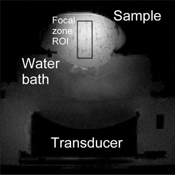
An MRI-compatible 256-element phased-array ultrasound transducer is housed in a waterbath, coupled to ex vivo porcine tissue samples. In-house-built surface coils are used for imaging.

Experiments

Thirty-nine separate HIFU heating runs were performed to test the MPF algorithm. For clarity, these experiments are named and summarized in Table 1.

Table 1.

Naming and Description of All 39 HIFU Heating Experiments

Experiment(s)	No. of runs	Sequence	Sampling	Power/duration	Notes
1.m	1	2-D GRE	Full	30 W/58.1 sec	For model identification
1.1–1.9	9	2-D GRE	Full	48 W/58.1 sec	All under identical conditions
2.m	2	2-D GRE	Full	27 W/58.1 sec	For model identification
2.A	8	2-D GRE	Full	36 W/58.1 sec
2.B	8	2-D GRE	R = 4.8	36 W/58.1 sec
2.C	8	3-D GRE	R = 12.1	36 W/58.1 sec
3.m	1	2-D GRE	Full	36 W/45 sec	For model identification
3.A	1	2-D GRE	R = 4.8	60 W/60 sec	Motion in two distinct moves
3.B	1	2-D GRE	R = 4.8	60 W/60 sec	Constant periodic motion

MPF With Retrospectively Undersampled Data Sets

In the first group of experiments (1.m and 1.1 through 1.9), parameter determination (run 1.m) was performed and then nine HIFU heating runs (1.1 through 1.9) were performed on an ex vivo tissue sample under identical circumstances, each imaged with the fully sampled 2-D GRE sequence. The nine fully sampled data sets were used for two purposes. The first was to determine the repeatability of the heating pattern produced by the ultrasound transducer under identical circumstances. The second purpose was to use the fully sampled temperature maps as truth in a comparison against MPF temperature maps created with retrospectively undersampled k-space data of increasing R factors.

To analyze the effect on the MPF temperature maps of using increasing reduction factors, undersampled data sets were created at various reduction factors by retrospectively zeroing out phase-encode lines from the fully sampled k-space sets. The seven reduction factors used were R = 2.6, 3.8, 4.8, 5.4, 6.3, 7.1, and infinite (model only using no measurements). For each reduction factor, the identified thermal model and the nine undersampled data sets were used in the MPF algorithm to create temperature maps.

MPF With Actually Undersampled Data Sets

The second group of experiments tested the performance of the MPF algorithm using actually undersampled data. After model identification, runs 2.A, 2.B, and 2.C were performed sequentially on a new ex vivo tissue sample, giving data sets of 2-D fully sampled images, 2-D undersampled images, and 3-D undersampled images, all done under identical conditions. This series of three heating runs was repeated three more times at the same location in the tissue sample, and then the transducer was moved, a new model was identified, and the same series of three heating runs was repeated four more times at the new location in the tissue sample. This provided eight temperature data sets for each of the three sequences, all performed under nearly identical conditions. The fully sampled 2-D sequence had a scan time of 8.3 sec compared to 1.8 sec for the undersampled 2-D sequence and 6.4 sec for the undersampled 3-D sequence. Because of these differences in time step, not every time frame matched up between the fully sampled and undersampled techniques. In order to properly compare the two temperature data sets, the model was used to forward predict the MPF temperatures by whatever time step was necessary at each frame to match up with the timing of the fully sampled temperatures.

MPF With Motion

The final group of experiments was performed to test the MPF algorithm in the presence of two types of rigid-body, translation-only motion. For these experiments, the 2-D undersampled sequence (R = 4.8) was used and heating was done on an agar gel phantom. In the first case (3.A), the sample was moved once during heating by approximately 6 mm in less than 2 sec and then moved again back to its original position during cooling. The referenceless phase subtraction method was used in the MPF algorithm for this data set. For the second case (3.B), the sample was under continuous periodic motion, with an amplitude of approximately 8 mm and a period of 8 sec. In this case, the phase subtraction was done using the look-up library method (36), for which 30 images were acquired during motion but before heating began.

Analysis

Two metrics were used to assess the MPF algorithm’s performance: (1) the average error of the MPF temperatures over the five hottest voxels in the focal zone at the hottest time frame and (2) a temperature root mean square error (RMSE). For both metrics, the fully sampled PRF temperatures were used as truth. To calculate the temperature RMSE, a 24 × 7 × 3-voxel region of interest (ROI) was considered over approximately 25 time frames. The spatial region covered all voxels that experienced significant heating (above ~4°C), and the number of time frames was chosen to cover all time frames of heating plus the steepest portion of the cooling phase. For the retrospective and prospective undersampling experiments, the average error of the five hottest voxels and the temperature RMSE were determined for all runs separately. The mean and standard deviation (SD) of these values over all of the runs were then calculated and are displayed in Table 2. In the case of the motion experiments, fully sampled PRF temperatures were not available to use as truth for comparison, thus allowing only a qualitative assessment.

Table 2.

Summary of Results for HIFU Heating Experiments^*

Comparison	Five hottest vox diff	RMSE
Mean (1.1–1.9), fully sampled vs model only	−0.1°C ± 0.9°C	0.83°C
Mean (1.1–1.9), fully sampled vs 1.1–1.9, fully sampled	0.2°C ± 1.0°C	0.38°C
1.1–1.9, fully sampled vs 1.1–1.9, MPF R = 2.6	0.4°C ± 0.1°C	0.22°C
1.1–1.9, fully sampled vs 1.1–1.9, MPF R = 4.8	0.8°C ± 0.4°C	0.29°C
1.1–1.9, fully sampled vs 1.1–1.9, MPF R = 7.1	0.8°C ± 0.5°C	0.33°C
2.A vs 2.B	−0.3°C ± 0.9°C	0.42°C
2.A vs 2.C	0.0°C ± 1.7°C	0.59°C

^*Temperature differences over the five hottest voxels in the hottest time frame and a temperature RMSE over a 24 × 7 × 3 × 25 ROI are displayed.

RESULTS

Model Performance

Figure 2a shows a comparison of temperatures of the single hottest voxel determined from the identified model only (R = infinite) and the corresponding mean and SD of the fully sampled PRF temperatures from experiments 1.1–1.9. The mean and SD of the temperature differences (fully sampled PRF model only) over a 24 × 7 × 3 ROI about the focal zone are shown in Fig. 2b. Without measurement data, the model alone overpredicts the temperatures during the heating phase by approximately 0.5°C on average. After more than 5 min of cooling, the model-only temperatures are hotter by an average of 1.7°C. Throughout all time frames, the SD of the temperature differences is never more than 0.7°C. The temperature differences over the five hottest voxels and the total RMSE are presented in Table 2 at the end of the Results section.

FIG. 2. Model performance.

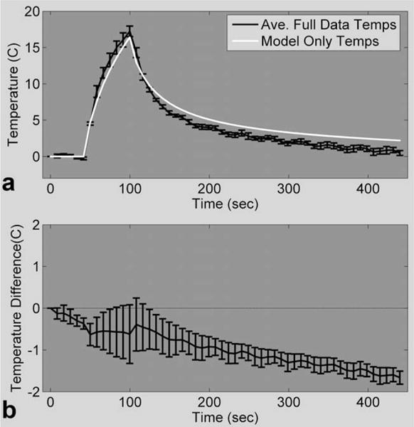
a: Temperature plot of one voxel in the focal zone comparing fully sampled PRF temperatures with model only temperatures for 48-W heating. b: Mean and SD of the model only temperature errors over a 24 × 7 × 3 ROI for all time frames.

Heating Repeatability With Fully Sampled Data Sets

The temperature measurements from the fully sampled data of heating runs 1.1 through 1.9 all had very similar temperature evolutions. From these nine heating runs, the average maximum temperature rise was 17.2 ± 0.7°C, ranging from 16.4°C to 18.3°C. The SD of the temperatures over all nine runs and all time frames in a 5 × 5 region that did not experience any heating was found to be 0.41 ± 0.02°C. Considering only the focal zone, the largest temperature SD was 1.2°C. To calculate the spread in the temperatures over the five hottest voxels and the total RMSE, the average of the nine temperatures was used as truth and compared against each individual run. These results are presented in Table 2.

MPF With Retrospectively Undersampled Data Sets

MPF temperature maps were created from retrospectively undersampled data for runs 1.1 to 1.9 and compared against the corresponding fully sampled PRF temperatures. As an example of the variations observed, Fig. 3 shows the mean and SD of the temperature differences over a 24 × 7 × 3 ROI covering the focal zone for run 1.3 at three reduction factors. The results for the MPF algorithm from the other eight heating runs were similar and indicate that the error is greater during times of rapid temperature change and appears to increase with reduction factor.

FIG. 3.

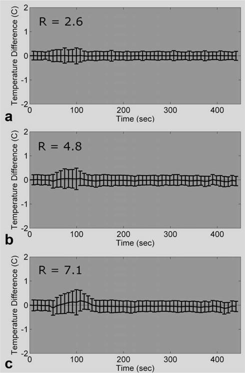
Comparing the MPF temperatures of run 1.3 versus the fully sampled PRF temperatures of run 1.3 (fully sampled PRF temperatures minus MPF temperatures; mean and SD over a 24 × 7 × 3 ROI). The temperature errors for the MPF algorithm at three different reduction factors are shown.

The mean and SDs of the temperature differences for the five hottest voxels were calculated for all nine heating runs at each of the six reduction factors, and the results are shown in Fig. 4a. Similarly, the MPF temperature RMSE was calculated for each heating run, and the mean and SD of the RMSEs are plotted as a function of reduction factor in Fig. 4b. These results are also summarized in Table 2.

FIG. 4. The error metrics as a function of reduction factor.

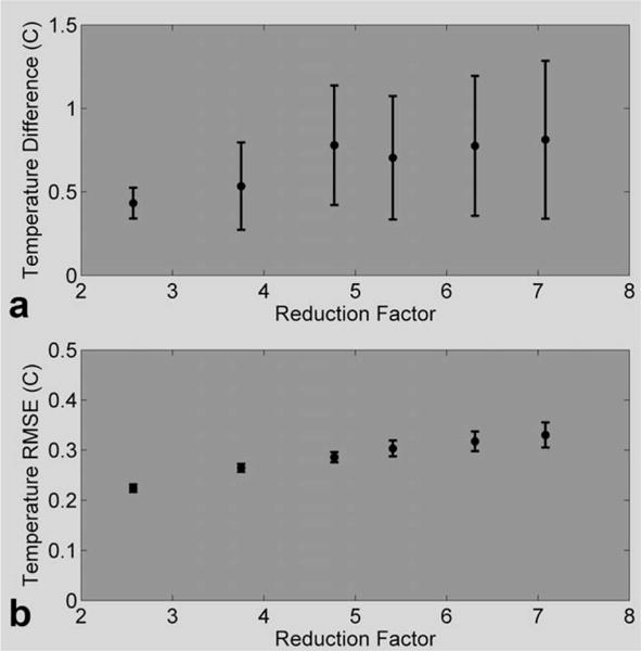
a: The error over the five hottest voxels in the hottest time frame (mean and SD over all 10 heating runs) at the six different reduction factors. b: Temperature RSME over a 24 × 7 × 3 × 25 ROI and all 10 heating runs at six different reduction factors.

MPF With Actually Undersampled Data Sets

Fully sampled PRF temperature maps from runs 2.A were compared to 2-D MPF temperature maps from runs 2.B. The maximum temperature rise measured over all of the 2.A runs had a mean and SD of 16.8 ± 1.7°C. For the corresponding 2-D MPF heating runs, the mean and SD of the maximum temperature rise were 17.0 ± 0.9°C. In Fig. 5a, the hottest voxel from the focal zone was chosen and the mean and SD over the four runs of the first location were plotted for each technique. For Fig. 5b, the temperature differences for these same runs were calculated over a 24 × 7 × 3 ROI, pooled together, and are displayed showing the mean and SD. The mean offsets are never larger than 0.4°C in either direction. The results for the four heating runs in the second location were similar. The temperature differences over the five hottest voxels and the total RMSE were calculated for all eight runs, and the results are summarized in Table 2.

FIG. 5. 2-D MPF temperatures compared to 2-D fully sampled temperatures.

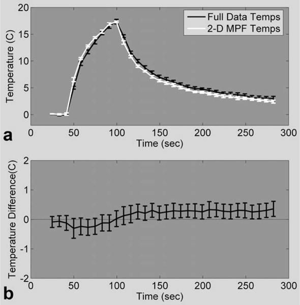
a: Mean and SD of the hottest voxel in the focal zone over the first four runs of fully sampled PRF temperatures (experiment 2.A, black line) and 2-D MPF temperatures (experiment 2.B, white line). b: Mean and SD of the temperature differences between runs 2.A and 2.B over a 24 × 7 × 3 ROI.

The same analysis was performed to compare the fully sampled PRF temperatures from runs 2.A to the 3-D MPF temperatures from runs 2.C. The maximum rise for the 3-D MPF temperatures ranged from 16.5°C to 18.0°C (mean, 17.2°C) for all of the 2.C runs. Results from the first four runs are shown in Fig. 6. The mean and SD of the temperature rise of a single voxel are shown in Fig. 6a (same voxel as displayed in Fig. 5a). The mean and SD of the temperature differences over the same 24 × 7 × 3 ROI are shown for all time frames in Fig. 6b. The mean difference fluctuates about zero but never rises above 0.2°C or falls below −0.4°C. The SD of the difference is larger than what was seen for the 2-D MPF temperatures, reaching 1.0°C for some time frames. Results for the second four heating runs were similar. The statistics for the temperature difference over the five hottest voxels and the total RMSE are shown in Table 2.

FIG. 6. 3-D MPF temperatures compared to 2-D fully sampled temperatures.

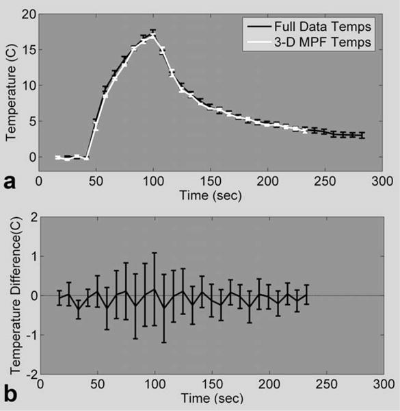
a: Mean and SD of the hottest voxel in the focal zone over the first four runs of fully sampled PRF temperatures (experiment 2.A black line) and 3-D MPF temperatures (experiment 2.C, white line). b: Mean and SD of temperature differences over a 24 × 7 × 3 ROI for all four runs.

MPF With Motion

Because no “true” temperature could be acquired for comparison against the MPF temperatures obtained in the presence of motion, only qualitative results can be given. Figure 7 displays results from run 3.A. In Fig. 7a, the three temperature-time curves are from one voxel in the center of the original focal zone and two voxels 6 mm to the right and left of this central voxel. The plot in Fig. 7b shows the displacement of the phantom that was calculated within the MPF algorithm for all time frames. The four temperature maps in Fig. 7c are from right before the first move, just after the first move, at the peak of heating, and just after the second move. Major artifacts occurred in one time frame during the first movement, causing large errors in the temperature maps. Other than this time frame, the temperatures calculated by the MPF algorithm behave as expected.

FIG. 7. 2-D undersampled MPF temperatures with discrete motion.

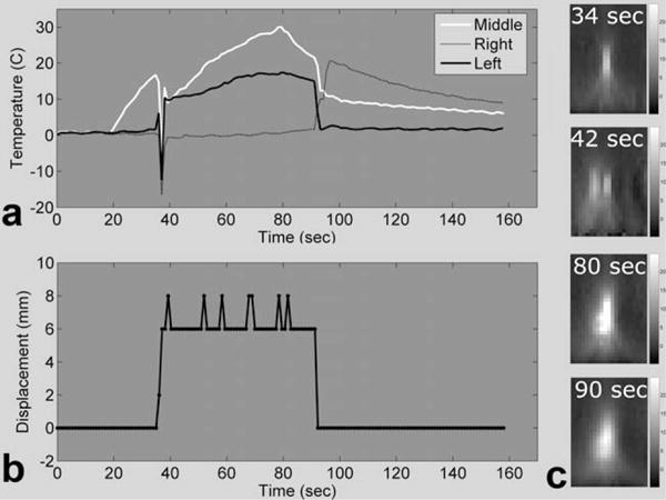
a: Temperature plots of three voxels in and near the focal zone, spaced 6 mm apart. b: Phantom displacement relative to the starting point, as measured by the method of Mendes et al. (33). c: Temperature maps showing the hot spot before moving, just after the first move, at peak heating, and just after the second move.

Figure 8 shows the MPF temperature results from the case of constant periodic motion. Temperature curves from voxels 6 mm to the right and left of the central focal zone are shown, along with the calculated displacement curve in Fig. 8a and b. Figure 8c shows four temperature maps covering one-half of a full oscillation period. In this case, the temperature maps had small artifacts in a number of the time frames due to the motion. For instance, negative temperatures can be seen in the far right side of the temperature map for time 96 sec, and some minor banding can be seen at the bottoms of the other three temperature maps. These artifacts were never severe but still most likely caused small errors in the calculated temperatures.

FIG. 8. 2-D undersampled MPF temperatures with continuous motion.

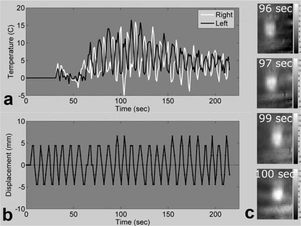
a: Temperature plots of two voxels in the focal zone, spaced 12 mm apart. b: Phantom displacement relative to the starting point, as measured by the method of Mendes et al. (33). c: Temperature maps showing the hot spot during heating at four consecutive times over one-half of a period.

MPF Robustness

Tests of the MPF algorithm’s stability with respect to model errors and noise were performed with the data from run 1.2. For the model error tests, varying degrees of error were introduced into the model prediction step by separately multiplying Q_rel, k, and ρ from Eq. 3 by a factor ranging from 0.5 to 1.5. The data were undersampled at R = 4.8 and these erroneous values were used in the algorithm to create MPF temperatures. The average error over the five hottest voxels, plotted as a function of the multiplication factor, is shown in Fig. 9a and a similar plot for temperature RMSE is shown in Fig. 9b.

FIG. 9. Evaluating the effect of model accuracy on the MPF algorithm.

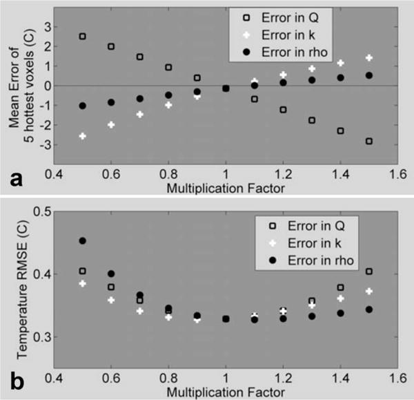
MPF temperatures were created using erroneous values for Q_rel, k, and ρ and were compared to fully sampled temperatures. a: Average difference over the five hottest voxels as a function of model error. b: Temperature RMSE over a 24 × 7 × 3 × 25 ROI as a function of model error.

To test the algorithm’s performance as a function of SNR, increasing amounts of randomly generated complex white noise were added to the originally acquired k-space data of run 1.2. For each of the different noise levels, temperatures were calculated from the fully sampled noisy data using the PRF method and from the noisy data undersampled at R = 4.8 using the MPF algorithm. For each noise level, this process was repeated 20 times and the average values for the reconstructed image SNR, the error over the five hottest voxels, and the temperature RMSE were calculated, using the original fully sampled data without noise as truth. The results are summarized in Table 3.

Table 3.

Summary of Results Comparing MPF and Full Data Temperature Maps as a Function of Image SNR Using k-Space Data From Run 1.2

Noise level (%of max k-space)	Image SNR		Five hottest voxels error		Temperature RMSE
	Full data	MPF (R = 4.8)	Full data	MPF (R = 4.8)	Full data	MPF (R = 4.8)
0.0	61.7	113.2	0.0 ± 0.0	−0.1 ± 0.4	0.0	0.3
0.1	53.2	102.3	0.0 ± 0.1	−0.1 ± 0.4	0.1	0.3
0.2	30.5	63.1	−0.1 ± 0.4	−0.2 ± 0.4	0.4	0.4
0.4	20.1	42.8	−0.1 ± 0.6	−0.2 ± 0.5	0.7	0.5
0.6	13.0	28.2	−0.1 ± 1.0	−0.2 ± 0.8	1.0	0.7
0.7	10.5	23.0	−0.2 ± 1.2	−0.2 ± 0.9	1.3	0.9
0.9	8.2	17.9	0.2 ± 1.6	−0.1 ± 1.0	1.7	1.1
1.1	7.1	15.6	0.1 ± 1.8	−0.3 ± 1.1	2.0	1.2
1.3	5.9	13.2	−0.1 ± 2.3	−0.1 ± 1.4	2.4	1.5
1.4	5.4	11.8	0.6 ± 2.5	0.1 ± 1.6	2.8	1.6

DISCUSSION

The work herein presents MPF, a novel method for accelerating scan time by reconstructing MR temperature maps from undersampled k-space data utilizing temperature predictions from a preidentified thermal model. The algorithm has been implemented for 2-D and 3-D versions of a radiofrequency spoiled gradient echo sequence. In each case, the pulse sequence has been modified to acquire undersampled data in real time at a user-determined data reduction factor. The MPF algorithm is recursive, with a computational burden small enough to allow for real-time applications. Although not demonstrated here, the MPF algorithm is sufficiently flexible to be used with any temperature-predicting model and any pulse sequence that acquires PRF data, including ones that incorporate segmented EPI readouts and reduced FOV imaging.

Over the course of 39 HIFU heating experiments, the performance of the MPF algorithm was compared against the current gold standard in MR temperature imaging, fully sampled 2-D PRF temperature images. The results summarized in Table 2 show that the MPF technique performed well, providing acceleration factors of 4.6 for the 2-D case and 12.1 for the 3-D case, with relatively small deviations from fully sampled 2-D PRF temperatures that were acquired under identical circumstances. Further results show that the MPF algorithm can monitor heating when motion is present, although the temperature errors are slightly worse, as would be expected.

In order to make temperature predictions using the Pennes bioheat equation, five different parameters must be set: ρ, C, k, Q, and W. Ideally, each of these parameters would be a spatially varying matrix with dimensions that match the MR images. However, identifying the spatial dependence of all of these variables is not an easy task to accomplish in practice and may not be necessary in all situations. In the studies presented here, the MPF algorithm was only tested with heat applied at a single point in relatively homogeneous, nonperfused ex vivo tissue and in a homogeneous phantom. Under these simple circumstances, the assumptions made were valid: ρ, C, and k were assumed to be scalars and constant over the ROI, the Q matrix was determined with heating at only one location, and W was set to zero. Our purpose here was to demonstrate the concept of how information from a thermal model could be combined with MR data to accelerate image acquisition. Further work is ongoing to demonstrate that the MPF algorithm can be applied in more clinically relevant circumstances. Note that this is an issue of improving the thermal model, not the MPF algorithm. Any refinement to the thermal model can be implemented directly into the MPF pipe line.

In its current state, the Q term needs to be identified at each new heating location. This is clearly not acceptable for an actual ablation procedure that would require sonications at numerous different locations. This problem is easily overcome for regions of homogeneous tissue (37) with mechanical transducer movement. The power deposition could be identified for one location and then extrapolated to the other locations based on knowledge of tissue ultrasound properties, thermal properties, and geometry. Another shortcoming is that the process used to determine ρ, C, and k is not currently able to identify multiple tissue types with varying properties. This may cause problems since all in vivo ablation procedures will involve at least two different tissue types. One likely solution will be to segment the MRI images and identify all relevant tissue types. Each tissue type will have density and specific heat assigned from table look-up values. The value for k could be identified as before in regions of aqueous tissue, but a look-up value would have to be used for adipose regions as MR temperature measurements in fat are not currently reliable. These additional steps will allow the thermal model to be applied to each region of different tissue types separately. A final area for improvement in the MPF algorithm is that it does not currently take into account temperature-dependent changes in the signal magnitude. Temperature changes will affect the tissue T₁, diffusion, and bulk magnetization. However, these changes will be sequence and tissue dependent and are not well established. Instead of trying to model the magnitude changes, which would likely be very complicated, we chose to use the magnitude from time frame N when predicting the k-space for time frame N + 1.

Because of tissue inhomogeneities and errors in thermal property measurements, the thermal model will never be perfect and some prediction errors will always remain. The effect of these errors should be relatively minor because the way that the MPF technique incorporates measured data makes it more robust to model error. The algorithm is similar to a sliding window reconstruction of undersampled data, with the important additional step of incorporating information from a thermal model. The central lines of k-space are sampled at every time frame, and they capture most of the phase information. When the tissue temperature is not changing rapidly, a sliding window reconstruction of undersampled data will give temperatures that closely match fully sampled temperatures. In areas where the tissue temperature is changing rapidly, sliding window temperatures will lag behind the actual temperature changes in time. It is in these locations that the thermal model is most needed. The strength of the model-only temperatures is that they do not lag behind the actual temperature changes. The controlling computer will always know when the ultrasound power is being turned on and off, and the model can use this knowledge to predict the temperature changes accordingly. When the model and data are combined into MPF temperatures, the errors are still largest during periods of rapid temperature change, although these errors are relatively small. Even at the largest reduction factors, the MPF algorithm predicts temperatures quite accurately during the first and last time frames shown, when the temperatures are not changing rapidly.

The results in Fig. 9 show that the algorithm’s performance is not significantly affected until the errors in the model parameters are large. It is likely that the MPF algorithm performance will be less affected by model inaccuracies and that errors will propagate less far in time when actually undersampled data are used. To have “true” temperatures for this analysis, fully sampled data were used that had a time step of 8.3 sec. When actually undersampled data are used, the model will be making predictions less far into the future, thus reducing its error. Additionally, large errors or erroneous predictions in the MPF temperatures should be detectable by comparing the measured k-space lines with the corresponding lines predicted by the model. Large differences between the measured and predicted k-space lines may be an indication of errors in the calculated temperatures. An appropriate correction could then be applied in real time, such as discounting the model for that time frame and only using the data in sliding window fashion.

The results obtained from subsampling the fully sampled measurements indicated an increase in error with increasing reduction factor. This increase is likely due to the fact that the time step between subsampled measurements did not decrease. In a real implementation, the time step will decrease as the reduction factor increases. With smaller time steps, the heat diffusion will be over a smaller volume, resulting in smaller footprint for the MPF kernel and a more stable propagation with increasing reduction factor. Thus, although the results of this paper provide strong evidence that the MPF algorithm can be used to greatly increase the temporal resolution in temperature measurements, more work is needed to establish the ultimate limits on accuracy as a function of reduction factor.

Although the undersampled MRI techniques used in these experiments do not achieve temperature measurements with 1 mm³ isotropic spatial resolution and 1-sec temporal resolution, this goal should be attained by combining the MPF algorithm with a segmented EPI readout and reduced FOV imaging. For example if an EPI readout factor of 6 were applied to the 3-D undersampled gradient echo sequence, the time resolution would become 1.1 sec. Adding 2-D radiofrequency excitation to decrease the FOV to 128 × 128 × 16 mm³ while keeping the acquisition matrix the same size would give 1 mm³ isotropic spatial resolution. As these strategies are independent, they can be combined to achieve the goal of 1 mm³/1 sec temporal and spatial resolution.

References

- 1.Mougenot C, Quesson B, de Senneville BD, de Oliveira PL, Sprinkhuizen S, Palussiere J, Grenier N, Moonen CT. Three-dimensional spatial and temporal temperature control with MR thermometry-guided focused ultrasound (MRgHIFU) Magn Reson Med. 2009;61:603–614. doi: 10.1002/mrm.21887. [DOI] [PubMed] [Google Scholar]
- 2.Wu F, Wang ZB, Chen WZ, Wang W, Gui Y, Zhang M, Zheng G, Zhou Y, Xu G, Li M, Zhang C, Ye H, Feng R. Extracorporeal high intensity focused ultrasound ablation in the treatment of 1038 patients with solid carcinomas in China: an overview. Ultrason Sonochem. 2004;11:149–154. doi: 10.1016/j.ultsonch.2004.01.011. [DOI] [PubMed] [Google Scholar]
- 3.Salomir R, Palussiere J, Vimeux FC, de Zwart JA, Quesson B, Gauchet M, Lelong P, Pergrale J, Grenier N, Moonen CT. Local hyperthermia with MR-guided focused ultrasound: spiral trajectory of the focal point optimized for temperature uniformity in the target region. J Magn Reson Imaging. 2000;12:571–583. doi: 10.1002/1522-2586(200010)12:4<571::aid-jmri9>3.0.co;2-2. [DOI] [PubMed] [Google Scholar]
- 4.Jolesz FA. Interventional magnetic resonance imaging, computed tomography, and ultrasound. Acad Radiol. 1995;2(suppl 2):S124–125. doi: 10.1016/s1076-6332(12)80051-1. [DOI] [PubMed] [Google Scholar]
- 5.Hynynen K, Damianou CA, Colucci V, Unger E, Cline HH, Jolesz FA. MR monitoring of focused ultrasonic surgery of renal cortex: experimental and simulation studies. J Magn Reson Imaging. 1995;5:259–266. doi: 10.1002/jmri.1880050306. [DOI] [PubMed] [Google Scholar]
- 6.Cline HE, Hynynen K, Watkins RD, Adams WJ, Schenck JF, Ettinger RH, Freund WR, Vetro JP, Jolesz FA. Focused US system for MR imaging-guided tumor ablation. Radiology. 1995;194:731–737. doi: 10.1148/radiology.194.3.7862971. [DOI] [PubMed] [Google Scholar]
- 7.Hynynen K, McDannold N. MRI guided and monitored focused ultrasound thermal ablation methods: a review of progress. Int J Hyperthermia. 2004;20:725–737. doi: 10.1080/02656730410001716597. [DOI] [PubMed] [Google Scholar]
- 8.Kennedy JE, Ter Haar GR, Cranston D. High intensity focused ultrasound: surgery of the future? Br J Radiol. 2003;76:590–599. doi: 10.1259/bjr/17150274. [DOI] [PubMed] [Google Scholar]
- 9.Denis de Senneville B, Quesson B, Moonen CT. Magnetic resonance temperature imaging. Int J Hyperthermia. 2005;21:515–531. doi: 10.1080/02656730500133785. [DOI] [PubMed] [Google Scholar]
- 10.Mougenot C, Salomir R, Palussiere J, Grenier N, Moonen CT. Automatic spatial and temporal temperature control for MR-guided focused ultrasound using fast 3D MR thermometry and multispiral trajectory of the focal point. Magn Reson Med. 2004;52:1005–1015. doi: 10.1002/mrm.20280. [DOI] [PubMed] [Google Scholar]
- 11.Carter DL, MacFall JR, Clegg ST, Wan X, Prescott DM, Charles HC, Samulski TV. Magnetic resonance thermometry during hyperthermia for human high-grade sarcoma. Int J Radiat Oncol Biol Phys. 1998;40:815–822. doi: 10.1016/s0360-3016(97)00855-9. [DOI] [PubMed] [Google Scholar]
- 12.Quesson B, de Zwart JA, Moonen CT. Magnetic resonance temperature imaging for guidance of thermotherapy. J Magn Reson Imaging. 2000;12:525–533. doi: 10.1002/1522-2586(200010)12:4<525::aid-jmri3>3.0.co;2-v. [DOI] [PubMed] [Google Scholar]
- 13.De Poorter J, De Wagter C, De Deene Y, Thomsen C, Stahlberg F, Achten E. Noninvasive MRI thermometry with the proton resonance frequency (PRF) method: in vivo results in human muscle. Magn Reson Med. 1995;33:74–81. doi: 10.1002/mrm.1910330111. [DOI] [PubMed] [Google Scholar]
- 14.McDannold N, Hynynen K, Wolf D, Wolf G, Jolesz FA. MRI evaluation of thermal ablation of tumors with focused ultrasound. J Magn Reson Imaging. 1998;8:91–100. doi: 10.1002/jmri.1880080119. [DOI] [PubMed] [Google Scholar]
- 15.McDannold N, Jolesz FA, Hynynen K. Determination of the optimal delay between sonifications during focused ultrasound surgery in rabbits by using MR imaging to monitor thermal build up in vivo. Radiology. 1999;211:419–426. doi: 10.1148/radiology.211.2.r99ma41419. [DOI] [PubMed] [Google Scholar]
- 16.Moonen CT, Liu G, van Gelderen P, Sobering G. A fast gradient-recalled MRI technique with increased sensitivity to dynamic susceptibility effects. Magn Reson Med. 1992;26:184–189. doi: 10.1002/mrm.1910260118. [DOI] [PubMed] [Google Scholar]
- 17.de Zwart JA, Vimeux FC, Delalande C, Canioni P, Moonen CT. Fast lipid-suppressed MR temperature mapping with echo-shifted gradient-echo imaging and spectral-spatial excitation. Magn Reson Med. 1999;42:53–59. doi: 10.1002/(sici)1522-2594(199907)42:1<53::aid-mrm9>3.0.co;2-s. [DOI] [PubMed] [Google Scholar]
- 18.Pruessmann KP, Weiger M, Scheidegger MB, Boesiger P. SENSE: sensitivity encoding for fast MRI. Magn Reson Med. 1999;42:952–962. [PubMed] [Google Scholar]
- 19.Sodickson DK, Manning WJ. Simultaneous acquisition of spatial harmonics (SMASH): fast imaging with radiofrequency coil arrays. Magn Reson Med. 1997;38:591–603. doi: 10.1002/mrm.1910380414. [DOI] [PubMed] [Google Scholar]
- 20.Madore B, Glover GH, Pelc NJ. Unaliasing by Fourier-encoding the overlaps using the temporal dimension (UNFOLD), applied to cardiac imaging and fMRI. Magn Reson Med. 1999;42:813–828. doi: 10.1002/(sici)1522-2594(199911)42:5<813::aid-mrm1>3.0.co;2-s. [DOI] [PubMed] [Google Scholar]
- 21.Tsao J, Boesiger P, Pruessmann KP. k-t BLAST and k-t SENSE: dynamic MRI with high frame rate exploiting spatiotemporal correlations. Magn Reson Med. 2003;50:1031–1042. doi: 10.1002/mrm.10611. [DOI] [PubMed] [Google Scholar]
- 22.van Vaals JJ, Brummer ME, Dixon WT, Tuithof HH, Engels H, Nelson RC, Gerety BM, Chezmar JL, den Boer JA. “Keyhole” method for accelerating imaging of contrast agent uptake. J Magn Reson Imaging. 1993;3:671–675. doi: 10.1002/jmri.1880030419. [DOI] [PubMed] [Google Scholar]
- 23.Webb AG, Liang ZP, Magin RL, Lauterbur PC. Applications of reduced-encoding MR imaging with generalized-series reconstruction (RIGR) J Magn Reson Imaging. 1993;3:925–928. doi: 10.1002/jmri.1880030622. [DOI] [PubMed] [Google Scholar]
- 24.Adluru G, Awate SP, Tasdizen T, Whitaker RT, Dibella EV. Temporally constrained reconstruction of dynamic cardiac perfusion MRI. Magn Reson Med. 2007;57:1027–1036. doi: 10.1002/mrm.21248. [DOI] [PubMed] [Google Scholar]
- 25.Rawnsley R, Roemer RB, Dutton AW. The simulation of discrete vessel effects in experimental hyperthermia. ASME J Biomechanical Engineering. 1994;116:256–262. doi: 10.1115/1.2895728. [DOI] [PubMed] [Google Scholar]
- 26.Moros EG, Dutton AW, Roemer RB, Burton M, Hynynen K. Experimental evaluation of two simple thermal models using hyperthermia in muscle in vivo. Int J Hyperthermia. 1993;9:581–598. doi: 10.3109/02656739309005054. [DOI] [PubMed] [Google Scholar]
- 27.Roemer R. Thermal dosimetry and treatment planning. In: Gautherie M, editor. Thermal dosimetry. Berlin: Springer; 1990. pp. 119–214. [Google Scholar]
- 28.Pennes H. Analysis of tissue and arterial blood temperatures in the resting human forearm. Appl Physiol. 1948;1:93–122. doi: 10.1152/jappl.1948.1.2.93. [DOI] [PubMed] [Google Scholar]
- 29.Chato JC, Lee RC. The future of biothermal engineering. In: Diller RK, editor. Heat and mass transfer in living systems. New York: New York Academy of Sciences; 1998. pp. 1–20. [DOI] [PubMed] [Google Scholar]
- 30.Roemer RB, Fletcher AM, Cetas TC. Obtaining local SAR and blood perfusion data from temperature measurements: steady state and transient techniques compared. Int J Radiat Oncol Biol Phys. 1985;11:1539–1550. doi: 10.1016/0360-3016(85)90343-8. [DOI] [PubMed] [Google Scholar]
- 31.Cheng HL, Plewes DB. Tissue thermal conductivity by magnetic resonance thermometry and focused ultrasound heating. J Magn Reson Imaging. 2002;16:598–609. doi: 10.1002/jmri.10199. [DOI] [PubMed] [Google Scholar]
- 32.Spiegel M. Mathematical handbook of formulas and tables. New York: McGraw-Hill; 1999. p. 278. [Google Scholar]
- 33.Mendes J, Kholmovski E, Parker DL. Rigid-body motion correction with self-navigation MRI. Magn Reson Med. 2009;61:739–747. doi: 10.1002/mrm.21883. [DOI] [PMC free article] [PubMed] [Google Scholar]
- 34.Peters RD, Hinks RS, Henkelman RM. Ex vivo tissue-type independence in proton-resonance frequency shift MR thermometry. Magn Reson Med. 1998;40:454–459. doi: 10.1002/mrm.1910400316. [DOI] [PubMed] [Google Scholar]
- 35.Rieke V, Vigen KK, Sommer G, Daniel BL, Pauly JM, Butts K. Referenceless PRF shift thermometry. Magn Reson Med. 2004;51:1223–1231. doi: 10.1002/mrm.20090. [DOI] [PubMed] [Google Scholar]
- 36.de Senneville BD, Mougenot C, Moonen CT. Real-time adaptive methods for treatment of mobile organs by MRI-controlled high-intensity focused ultrasound. Magn Reson Med. 2007;57:319–330. doi: 10.1002/mrm.21124. [DOI] [PubMed] [Google Scholar]
- 37.Blankespoor A, Todd N, Goodrich KC, Moellmer J, Parker DL, Roemer RB, Skliar M. International Symposium on Therapeutic Ultrasound. Seoul; South Korea: 2007. Model predictive control of minimal time, phased array HIFU treatments. [Google Scholar]