Structured states of disordered proteins from genomic sequences

SUMMARY

Protein flexibility ranges from simple hinge movements to functional disorder. Around half of all human proteins contain apparently disordered regions, with little 3D or functional information, and many of these proteins are associated with disease. Building on the evolutionary couplings approach previously successful in predicting 3D states of ordered proteins and RNA, we developed a method to predict the potential for ordered states for all apparently disordered proteins with sufficiently rich evolutionary information. The approach is highly accurate (79%) for residue interactions as tested in over 60 known disordered regions captured in a bound or specific condition. Assessing the potential for structure of over 1000 apparently-disordered regions of human proteins reveals a continuum of structural order with at least 50% with clear propensity for three- or two-dimensional states. Co-evolutionary constraints reveal hitherto unseen structure of functional importance in apparently disordered proteins.

ETOC blurb

Sequence co-variation shines a light on structural states in flexible and disordered proteins

INTRODUCTION

Many, if not most, proteins can adopt alternative functional conformations and around half of all human proteins contain regions of at least 40 residues classified as disordered by a number of different bioinformatic methods (Oates et al., 2013; van der Lee et al., 2014) (Figure 1; Table S1) including many transcription factors with hundreds of so-called disordered regions. Conformational heterogeneity has long been recognized as necessary for protein function (Koshland, 1959; Monod et al., 1963; Perutz, 1970) and is associated with diverse cellular functions including metabolism, gene regulation, signaling, and molecular transport, spurring growing interest in so-called disordered and low-complexity sequences (Bah et al., 2015; Ferreon et al., 2013; Motlagh et al., 2014; Tokuriki and Tawfik, 2009; Uversky and Dunker, 2010; Wells et al., 2008; Wright and Dyson, 2015). Most recently, low complexity sequences have also been associated with physiological prion-like polymers that form hydrogels and membrane-less compartments, such as Fus and hnRNPA2 (Hyman et al., 2014; Kato et al., 2012; Kwon et al., 2013; Patel et al., 2015). However, protein flexibility is also associated with pathologies characterized by alternative folding or illicit polymerization, such as cancer, diabetes, and neurodegenerative disorders (Knowles et al., 2014; Lorenzo et al., 1994; Patel et al., 2015) and it remains unclear how much these alternate states may have physiological functions.

Figure 1. Co-evolutionary analysis of disordered segments in the human proteome.

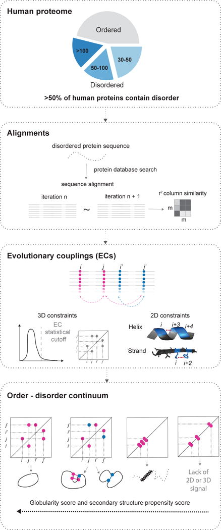
First we identify contiguous regions of disorder, secondly we search for similar sequences and select robust alignments; thirdly we calculate evolutionary couplings for each alignment using an updated algorithm to compute significant long range ECs and secondary structure propensity from short-range ECs. Finally we assess these predictions to reveal the likelihood of secondary and tertiary structure (Experimental Procedures).

Unfortunately, the flexibility of proteins is a challenge for traditional and even state-of-the-art methods of experimental and computational investigation. This leaves many of their functions and 3D structures out of reach, which is particularly frustrating as these proteins are at the heart of very active areas of research. Bioinformatic algorithms that predict disorder are typically based on sequence bias that has in turn been learnt from experimental evidence from CD or NMR spectra (Alexander et al., 2009; Knowles et al., 2014; Mittag et al., 2008; Sambashivan et al., 2005; Tokuriki and Tawfik, 2009; Tompa, 2002; Uversky and Dunker, 2010; Wells et al., 2008; Wright and Dyson, 2015). A small minority of proteins considered disordered have been observed experimentally and sample from a spectrum of structured-ness. These observations range from seeing solely secondary structure propensity (Fuxreiter et al., 2004; Uversky et al., 2002), to transient ensembles, through to more stable order in specific conditions, for instance when binding a ligand, a protein, DNA, RNA or post-translational modification (Bah et al., 2015; Baker et al., 2007; Hurley et al., 2007; Tompa and Fuxreiter, 2008).

However, except for a tiny percentage of cases (~ 1%), we do not know whether apparently disordered proteins can take on ordered states in vivo (Frederick et al., 2015) and the conditions for functional and structural experiments are unlikely to be known a priori for the vast majority. In the extreme, so-called fuzzy complexes have functional disordered regions that have been confirmed even when in their bound states (Tompa and Fuxreiter, 2008). Whilst it is possible that some disordered regions of proteins remain intrinsically disordered in all of their physiological states (Guharoy et al., 2015), there may be many disordered regions that have specific, but as yet uncharacterized, conformations in vivo.

By exploiting recent advances in predicting tertiary contacts and 3D structures from sequence alignments, we sought to uncover what evolutionary information from protein sequences alone could reveal about 2D and 3D structural states of low complexity sequences or proteins considered disordered (Hopf et al., 2012; Livesay et al., 2012; Marks et al., 2011; Morcos et al., 2013; Morcos et al., 2011; Thompson and Baker, 2011; Weinreb et al., 2016). We made no assumption that the proteins or regions take on any structural constraint in vivo and used co-evolutionary analysis of thousands of genomic sequences to predict the likelihood of structural constraints of the human disordered proteome. The approach builds on recent successful attempts to predict 3D structures from natural sequence variation (Hopf et al., 2012; Hopf et al., 2014; Marks et al., 2011; Morcos et al., 2013; Ovchinnikov et al., 2014; Weinreb et al., 2016) and here we develop statistical methods crucial for the applicability to low-complexity sequences. Although we, and others, have reported alternative residue contacts for alternative states (Hopf et al., 2012; Morcos et al., 2013), this is the first report of a systematic exploration of alternative and disordered states in the human proteome.

Here, we develop the evolutionary coupling method to analyze protein sequences predicted or known to be disordered. We first present the results of the method for a set of disordered proteins that have experimental evidence of their structural states (retrospective prediction set) and follow this with de novo predictions for a set of apparently-disordered regions that were assembled from all human proteins. Our computational inference is based only on sequence co-variation, identifies accurate secondary (2D) and tertiary (globular, 3D) structural constraints for the retrospective set and predicts evidence of structural constraints for over 90% of disordered regions in the human proteome that are currently amenable to the method.

RESULTS

Method development

We surveyed all human proteins for disorder using standard methods (Dosztanyi et al., 2005) finding that around 50% of human proteins have disordered regions of more than 30 residues, with 3585 proteins containing 4543 continuous disordered segments longer than 100 residues (Figures 1 and S1; Table S1; Experimental Procedures). Some of these proteins may have 3D structures in specific conditions, or alternatively exist in an ensemble of states in any single condition.

In order to compute the structural propensity, we developed the evolutionary couplings method in three areas: (i) Sequence alignments. After conducting systematic iterative alignments using jackhammer (Johnson et al., 2010) we found 1469 (32%) segments recovered sufficient numbers of similar sequences (> 5L sequences after redundancy reduction, where L is the length of the sequence) and coverage to move forward with the analysis. However, many of the alignments looked as though they may be arbitrary, which is to be expected when there are high substitution rates (Brown et al., 2010) and low-complexity amino acid composition that is one of the hallmarks of disorder classification. Since success of the co-evolutionary model for residue interactions depends critically on the quality of the sequence alignment, the challenge here was to develop criteria that measure alignment uncertainty. We therefore developed a pipeline that fetches and aligns sequences across a range of parameters, requiring a stable alignment as a condition for coupling calculations. The alignment robustness score represents the agreement of the amino acid composition of the alignment columns after different rounds of re-alignment iterations.(Figures 1 and S1). (ii) EC inference and statistical score. We modified our previously published method for determining accurate 3D constraints from sequences (Hopf et al., 2014; Marks et al., 2011; Morcos et al., 2011) so that gaps in the sequence alignment are excluded in the calculation in a self-consistent way. Gap removal is particularly critical for the evaluation of local, short range, evolutionary couplings that are otherwise dominated by noise created by gap-gap correlations. To assess the quality of the inferred evolutionary couplings we defined a statistical confidence measure based on the EC score distribution (without using any structural information). The distribution is approximated by a Gaussian-lognormal mixture model and we defined the tail of the distribution as those scores that have >90% probability of belonging to the lognormal component. ECs in this tail are defined as high probability. (iii) Fold probability. We assessed how likely the protein (or region) was to have some three-dimensional fold(s) by using the number of high probability long-range ECs computed from the alignment, in proportion to the length. Similarly, we identified propensity towards secondary structures in disordered proteins without relying on standard secondary structure prediction methods (Yachdav et al., 2014) as these are trained on predominantly ordered sequences. Here we considered the relative strength of local ECs ((i to i+3) and (i to i+4) for α-helices, and (i to i+2) for β-strands) (Figure S2A).

Retrospective prediction: ECs capture known states of structural plasticity

We next tested, completely blindly, whether evolutionary couplings can capture the secondary (2D) and tertiary (globular, 3D) states of proteins that have been observed in an ordered conformation but also have experimental evidence of disorder. We assembled a set of 83 proteins that contain disordered regions (45 proteins) or conformational changes (38 proteins) and have robust alignments - an additional 13 disordered regions were filtered out based on our alignment quality criteria (Table S2). These proteins included examples ranging from relatively simple conformational changes to those with evidence of complete disorder unless bound to a ligand or partner. Over all the proteins tested 79% of the ECs were close in the corresponding known structures (Figure 2A, Figure S2B), which is comparable to the prediction accuracy for ECs of well-ordered proteins previously published (Marks et al., 2011), and 97% (37/38) of the proteins with known alternative conformations have high confidence ECs that correspond to contacts unique to at least one conformation (Figure S3A, Table S2A). Since the secondary structure prediction approach is novel, we tested our method blindly on over 2800 independent domain families with known structures resulting in precisions of 86% for α-helices and 52% for β-strands (Figure 2A; Table S3). We noted that we tend to over-predict β-strands, which could be due to a combination of under-annotation, multimer signals, and less evolutionary constraint.

Figure 2. Experimentally determined states of flexible proteins are captured by evolutionary couplings.

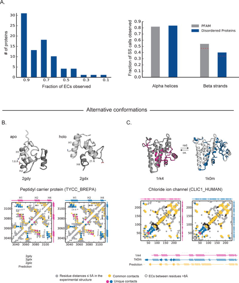
(A) Overall performance predicting experimental contacts for a set of 83 flexible and disordered proteins with known structures for significant long-range ECs (left panel) and precision of the secondary structure propensity scores on a per residue basis for a set of over 3800 PFAM families and our validation set of 83 flexible and disordered proteins with known structures (right panel). For residues with a propensity score suggesting both α-helix and β-strand we took these residues to be α-helical given stronger evolutionary constraint; red-dashed lines show the decreased precision including these calls in β-strand as well. (B) Peptidyl carrier protein (PCP) undergoes large conformational changes, including the repacking of its helices, upon cofactor binding (left: apo form, 2gdy; right: holo form, 2gdx). ECs reflect interactions between helix1 and helix2 (magenta circle, only in apo 3D structure) as well as helix1 and helix4 (blue circle, only in holo 3D structure). Many residue-residue distances change substantially between the two conformations. For example, there is strong coupling between residues K18 and E58, which form a salt bridge in the apo form, while they are >20 Å apart in the holo form. Our secondary structure propensity score predicts all 4 helices of PCP, the third being present only in the intermediate state between the apo and holo form (2gdw). (C) ECs agree with a known conformational switch in the chloride ion channel protein (CLIC1) undergoes redox condition dependent conformational switch, including α-helix to β-strand transitions.

Alternative states

Our EC approach successfully predicts alternative structural states. The peptidyl carrier protein (PCP) undergoes large conformational changes when it binds its cofactor, 4′-phosphopantheine, resulting in two distinct states that have been captured by NMR (Koglin et al., 2006). The ECs capture contacts that remain the same in the two structures, those that are unique to the holo, co-factor bound form (16 pairs), and those unique to the apo-form of PCP (5 pairs), (Figures 2B and S3A). Folding the protein with the EVfold pipeline results in a structure similar to an average of the 2 structures, and most similar to a 3^rd structure where the protein is captured in a transition state (PDB: 2gdz (Koglin et al., 2006)). In contrast folding PCP using ECs that are satisfied in all conformations together with those unique to each structure in turn gives 3D all-atom structures that are 2.5–3 Å C_α rmsd from each of the respective crystal structures (PDB: 2gdy (Koglin et al., 2006) (apo) and PDB: 2gdx (Koglin et al., 2006) (holo)). This shows that the respective ECs are sufficient to constrain the specific alternate functional fold. Correspondingly, local ECs capture alternative secondary structure elements. With PCP, ECs predict helix 3 (H3) that is unique to the transition state (Figure 2B) and strand and helix alternatives in the Chloride intracellular channel protein (CLIC1) (Figures 2C and S3C).

Disorder to 2D and 3D

Next, we tested the ability of the method to identify 2D and 3D contacts of disordered proteins that have been observed in specific conditions. Most of the significant ECs matched residues that were close in the observed conformations (Figure S4; Table S2B). Two of the most accurate predictions were for the disordered domain of the transcription factor Lef-1 (Love et al., 2004) where ECs perfectly recapitulate 73 contacts of the folded state (Figure 3A) and for the disordered domain of the chaperone Calnexin, where ECs recapitulate contacts observed in the crystal structure (Schrag et al., 2001; Williams, 2006) in the extended arm of a chaperone wrapping around the substrate molecule, including the observed β-strands⁴³ (Figure 3B).

Figure 3. Evolutionary couplings predict close residues in known ordered states of disordered proteins.

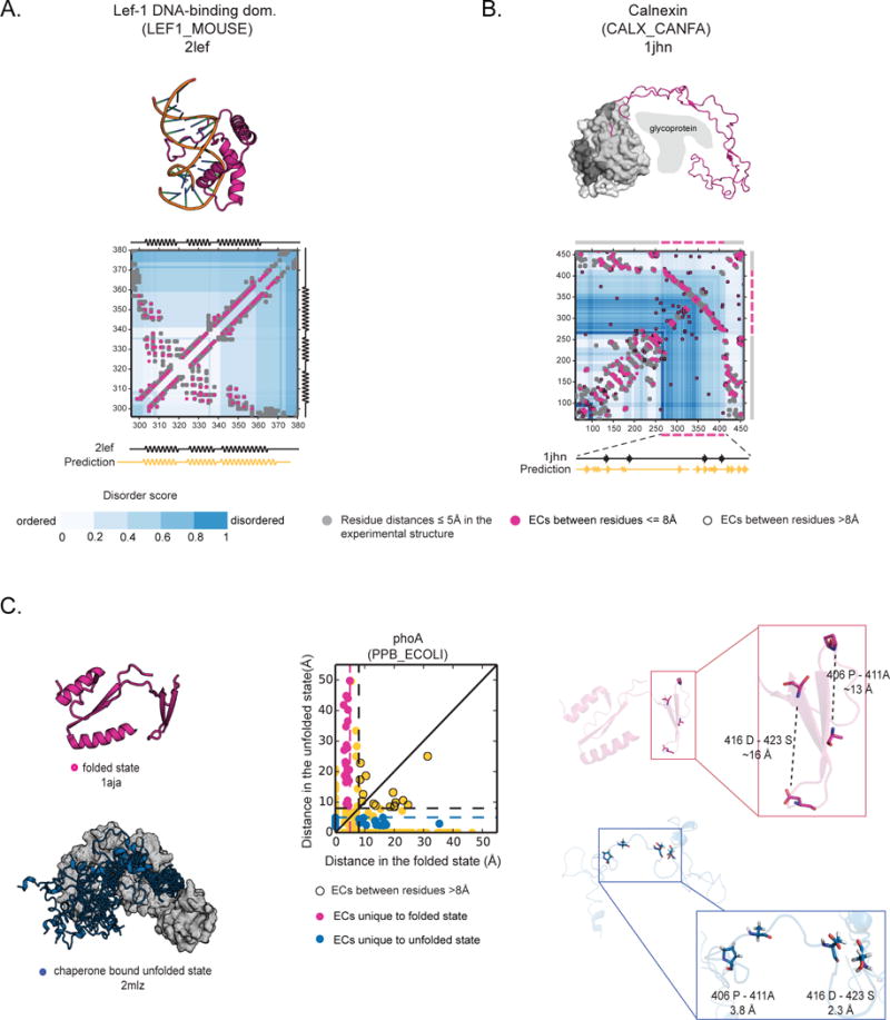
(A) ECs (pink circles) perfectly recapitulate the experimental contacts (grey circles- residue-residue distance <5 Å) of the folded, DNA-bound state of Lef-1 that is partially unstructured in the absence of DNA (2lef, Precision=1.00). (B) ECs predict the overall contact map of Calnexin chaperone, including the disordered luminal domain, which only folds when binding unfolded glycoprotein (1jhn, Precision=0.58). (C) phoA has been captured experimentally in the folded state (1aja) and unfolded state when bound to a chaperone (2mlz) (left panel). ECs capture contacts that are unique to the folded state (pink circles) and some unique to the unfolded state (blue circles) (middle panel). Specifically two pairs of ECs predict residue pairs that are only close in the “unfolded” state (between 416D-423S, and 406P-411A, ~16 and ~13 Å apart in the folded state and 3.8 and 2 Å apart in the unfolded state) (right panel).

In the third example, we were able to identify 3D contacts arising during chaperone bound folding of phoA, the dynamics of which were recently captured using state-of-art relaxation NMR experiments (2mlx/y/z (Saio et al., 2014)). In the reducing environment of the cytosol, phoA is disordered (Saio et al., 2014) and it only folds when oxidized. The alignment of ~ 3095 sequences had 111 significant ECs, coinciding largely with contacts in the globular, oxidized structures (PDB: 1aja (Dealwis et al., 1995)). However, there are also 3 pairs of significant ECs for contacts that are made only in the chaperone bound “unfolded state” and that are more distant in the folded protein (Figure 3C). These results suggest that this chaperone bound state seen in the NMR experiments may be under selection.

Since some disordered proteins are known to have folds when they co-fold with their binding partners, we also tested whether the signal from ECs was improved by using a joint multiple sequence alignment of a pair of proteins that bind, specifically in the case of anti-σ factor FlgM bound to σ ²⁸(Sorenson et al., 2004). The ECs calculated on the whole complex alignment, rather than on FlgM alone, more accurately capture FlgM’s internal contacts suggesting that the information for the structured fold of FlgM is partly encoded in the protein’s partner, σ²⁸ (Figure S5). This observation has implications for de novo, real world predictions suggesting caution on the interpretation of a lack of signal for either secondary or tertiary contacts; i.e. structured states may exist, but be invisible to evolutionary coupling analysis unless the biomolecular partner is included in the statistical analysis. Despite the high correspondence of EC pairs to observed close residues, there are some significant ECs involving residue pairs that are not close in the experimentally captured states (~ 20%, Figure 2A and Table S2). These false positives may reflect constraints that are not the result of monomeric residue proximity, for instance multimers, ligand and other biomolecular interactions as discussed in previous work (Marks et al., 2011). It remains to be seen if these represent ‘true’ false positives or residues that are close in, as yet, unseen conformations and In a two of the cases seen here, there is additional experimental support for these putative alternative states suggested by the ECs (Figure 4).

Figure 4. EVFold predictions of novel states of disordered proteins.

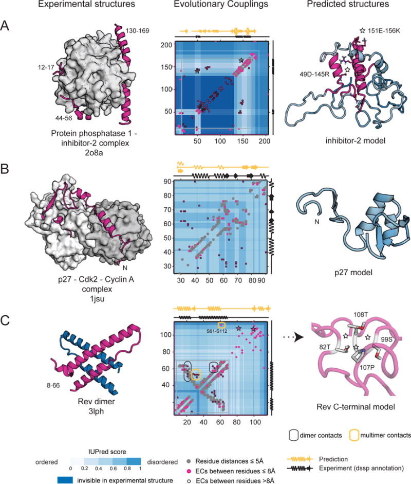
(A) Protein phosphatase 1 inhibitor 2 (IPP2_MOUSE), a disordered regulator, binds to its complex partner via three anchoring regions (residues12–17, 44–56, and 148–151), while the rest of the molecule remains invisible in the crystal structure (blue shading). ECs predict the existence of the helical anchors, as well as the long-range interactions between these regions. (B) Predicted contact map of p27 (CDN1B_HUMAN) reveals alternative states that are not compatible with the bound structure, and might form when free or bound to another partner. (C) Rev protein of HIV (REV_HV1H3) was captured experimentally in a dimeric state that is corroborated by the EC map, which has contacts for the helix-helix packing and the dimer contacts of the experimental structure (3lph). Additionally, possible multimer contacts may explain the higher order oligomerization of Rev. The C-terminal, invisible in experiments thus far, has signal for helical structure and has long-range evolutionary constraints indicative of a folded state (predicted 3D model, C, right).

Some proteins may have additional states

Some proteins in the validation set have ECs that suggest an additional structural state. To be conservative we still count these ECS as false positives in the overall evaluation even though some have evidence for additional as yet unobserved states. A few high ranked ECs in the protein phosphatase inhibitor II (PPI2) are between residues distant in the structure of the bound inhibitor (PDB: 2o8a (Hurley et al., 2007)), but consistent with observations made in NMR studies of its free state, where contacts between regions 140–150 and 65–75 are observed (Dancheck et al., 2008; Marsh and Forman-Kay, 2012) (Figure 4A). Similarly, ECs between the two helices of the LH domain in the disordered p27^KIP1 protein (a cyclin dependent kinase inhibitor) are distant in the structure of p27^KIP1 bound to cyclin A (PDB: 1jsu (Russo et al., 1996)) (Figure 4B). However the regular pattern of consecutive pairs suggests the antiparallel helical-packing arrangement is evolutionarily conserved.

The ECs for the HIV Rev protein recapitulate the known 3D structure of the N terminal region, including multimer contacts seen in a number of experimental structures (Daugherty et al., 2010; Jayaraman et al., 2014) (black and yellow ovals, Figure 4C). This includes a number of pairs (e.g. F21-R58) that are only close when Rev is bound to the RRE (Rev response element) in HIV (Daugherty et al., 2010; Jayaraman et al., 2014). A high ranked EC residue pair between the N and C-terminal domains, S61-S112, and a number of other clustered ECs are consistent with additional multimer contacts (yellow ovals, Figure 4C). We also predict ECs that form a network of tertiary contacts and well-defined secondary structure in the C terminal region of Rev – so far unseen in experimental structures.

To explore possible 3D states of p27, PPI2 and Rev we computed 3D models using distance constraints from long range ECs and secondary structure prediction from local ECs. These predicted structures have EC-derived contacts that could be salt-bridges, and in the case of PPI2 bring together a region close to the putative phosphorylation switch.

No 3D signal

PSMD4 (Rpn10/S5a) is a di-ubiquitin binding protein and part of the 19S regulatory proteasome that captures substrates with two ubiquitin-interacting motifs (UIMs). None of the contacts that we predict are long range, agreeing with the NMR structures of PSMD4 bound to di-ubiquitin (PDB: 2kde (Zhang et al., 2009)) (Dikic et al., 2009). Nevertheless our short range ECs predict the α-helices of PSMD4 seen in the NMR structures and the top two ECs (Q292-Q296, A290-S294) of PSMD4 lie in a helical segment that binds ubiquitin (Figure 5A) (Walters, 2005), suggesting that local enrichment of couplings can capture functional residues in this disordered domain. Intrinsically disordered bovine HMGN2 has been explored using methyl-based NMR to assess its binding to histones and DNA (Kato et al., 2011) and we do not see signal for long distance contacts in this region despite a signal for some β-strands. Similarly, there is an absence of 3D signal in the C-terminal end (110–210) of the H1.0 histone while we accurately predict 3D and 2D signal from ECs in the N terminal region (42–110) matching the known structure of the linker histone domain (PDB: 1ghc (Cerf et al., 1994)) (Figure 5B). In summary, this set of retrospective predictions (83 protein regions), demonstrates both that high-confidence ECs are generally accurate whether in 3D or 2D and that the lack of 3D signal from ECs often coincides with proteins where experimental evidence supports the lack of definable structure (Figures S4 and S5; Tables S2 and S3).

Figure 5. Accurate prediction of structure without long-range contacts.

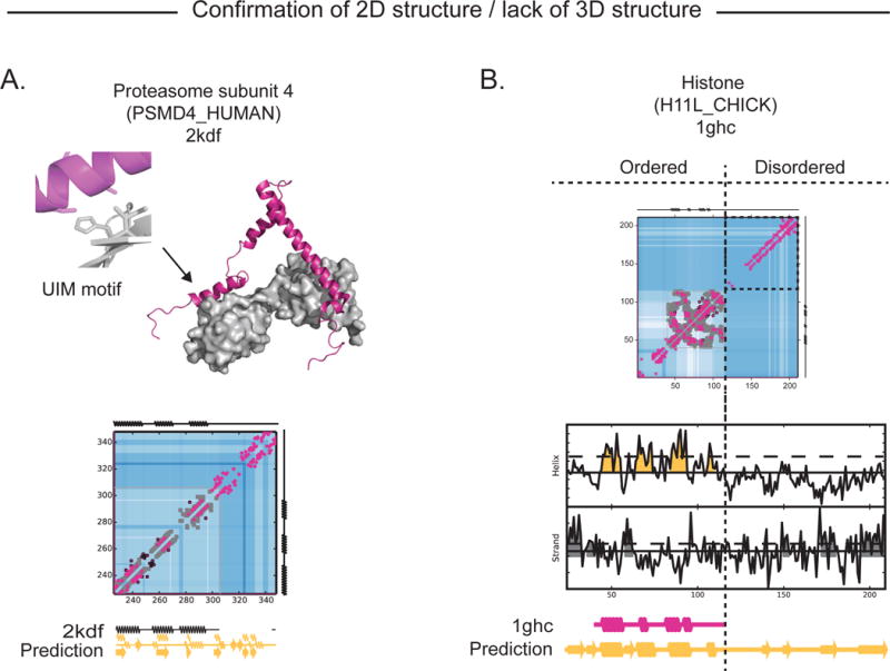
(A) The experimental 3D structure of PSMD4 in complex with di-ubiquitin (2kdf) has no long range contacts between the helices ensuring he separation of the two ubiquitin interacting motifs (UIMs) (top). Consistent with this, there are no ECs between residues distance in chain but nevertheless local ECs identify the helices formed when bound to ubiquitin as well as a weaker signal for possible β-strands. (B) ECs (pink circles) match the known contacts (grey circles) in the structure of the N terminal end of the histone H1.1 (1ghc, (P08287)) but do not predict long-in-chain contacts in the C terminal tail, consistent with observations that the histone tail is flexible in vivo. Secondary structure prediction of C terminal region suggest β-strands.

Evolutionary signal for amyloid and non-native states

For the functional amyloid curlin, csgA, in E. coli we see strong secondary structure propensity signal for β-strands along the length. Here, long-range significant ECs match previously predicted pairs of β-sheet hydrogen-bonded residues in the amyloid of csgA (Tian et al., 2015). We cannot exclude the possibility that some of the evolutionary constraints that lie in parallel to the diagonal are artifacts of the repeat nature of the sequences. Nevertheless, additional, antiparallel clusters of ECs in the middle of each repeat together with β-strand signal from local ECs are consistent with previously proposed amyloid organization (Figures S6) (Tian et al., 2015). Similarly, there is a distinctive pattern of ECs in the N terminal disordered region of FUS, a gene associated with both oncogenesis and the pathogenesis of amyotrophic lateral sclerosis (ALS). Local ECs predict β-strands consistent with reports that this region may have a propensity to form functional β-strand fibrils (Figure S6) (Kato et al., 2012). In contrast, ECs predict only α-helical secondary structure for alpha-synuclein, and no strong β-strand propensity. This prediction is therefore not in agreement with a β-hairpin observed in a structure of alpha-synuclein observed bound to an engineered protein (PDB ID: 4bxl (Mirecka et al., 2014)). However, our prediction is in agreement with the α-helices seen in most of the structural experiments including the micelle-bound, partially folded conformations of alpha-synuclein captured by NMR and EPR (PDB ID: 2kkw (Rao et al., 2010)) (Figure S6). These results suggest that evolutionary information may be useful to explore the propensity of amyloid formation and further work should specialize in determining signals for higher order structure formation.

Screening the human disordered proteome

3D contacts predicted

32% of the disordered regions we identified for exploration had sufficient number of sequences, enough diversity and good coverage (M_eff > 5 per residue) resulting in 1469 segments, of which 965 had robust alignments (Figure 6A, Table S4). The majority (92%) of this set of 965 regions have evolutionary signal for 2D or 3D structural constraints, and roughly 42% have significant long-range ECs that indicate a constrained 3D fold or folds. 8% do not show signal for structure despite having sufficient sequences and robust alignments (Figures 6A, 6B, and 6C). For a small subset of proteins (33) with 3D contacts, there is a related sequence with known 3D structure for part of the disordered query region - but the remaining most likely represent de novo predictions of 3D contacts of proteins that have been previously considered as disordered.

Figure 6. Human proteome wide prediction of structural states of disordered proteins.

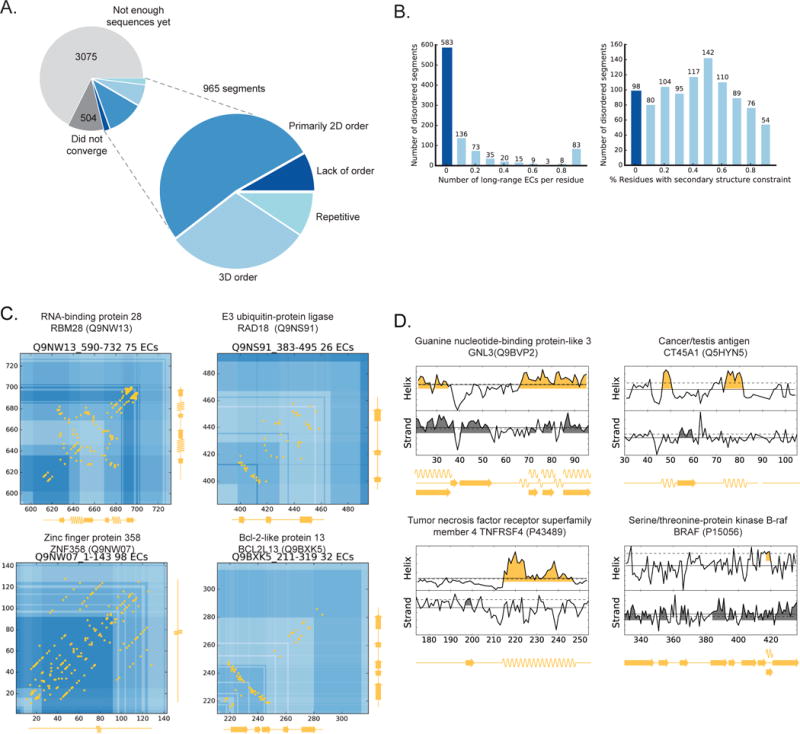
(A) Out of the 4543 disordered segments analyzed, 21% (965) of these had alignments with sufficent sequences that also met our convergence criteria. 381 (40%) of these segments have long-range ECs giving a globularity score >0.1), another 52% have predicted 2D constraints (secondary structure propensity score >0.1) but very few 3D constraints, and the remaining 8% show almost no signal for any structural constraints. Almost 10% also have EC patterns suggestive of repeats. (B) Distribution of long-range predicted contacts (left) and the propensity to secondary structure (right) across the proteins. (C) Four examples of proteins with high proportion of long-range ECs (yellow) that have no known structure and are considered disordered. Secondary structure predictions (yellow along axes) correspond well to tertiary structure packing indicated by the long range ECs. (D) Four examples of proteins without evidence of a 3D contacts, but that do have with predicted secondary structure elements. All of our predictions and data files are available on the web at marks.hms.harvard.edu/disorder/.

381 protein regions have high 3D signals (more than 0.1L long-range ECs, (where L=length of disordered region) including regions in an RNA binding protein, RBM28 (Q9NW13), a DNA repair protein, RAD28 (Q9NS91), a zinc-finger protein, ZNF358 (Q9NW07), and a Bcl-2-like protein (Q9BXK5) (Figure 6C). The longer range ECs are clustered in a way that is typical of secondary structure 3D packing, and correspond to the independently computed secondary structural elements from the local EC scores. In many examples, the contacts resemble those from 3D folds related to the known function of the whole protein. For instance for some proteins containing annotated zinc-fingers, the predicted contacts of the unknown regions resemble zinc finger motifs and the ECs of a disordered region of RBM28 resemble a typical RNA–binding domain.

Since we find that a significant proportion of these regions have secondary or tertiary predicted contacts, we wondered whether the regions in our set that retrieved enough sequences may be biased towards structured-ness. We do indeed find that the extent of predicted disorder is somewhat shifted between our computed set and the set of the remaining regions that had insufficient sequences or non-robust alignments. However, the bias is small; for example 72% of the computed set versus 82% of non computed set have disorder scores > 0.6. (Figure S2B). In addition we do not see bias towards less disorder with those regions that have clearer 3D signal. Around 90 proteins have a large proportion of significant ECs that are long in chain distance resulting in globularity scores higher than one might expect from a typical globular fold. In theory these could be due to multimer contacts but are more likely to be a signature of repeats that will result in couplings between residues in multiples of the lengths of the repeats. We expect to develop the method to deconvolute these signals in future work.

Regions with primarily secondary structure

505 regions have very few, if any, long-range contacts but nevertheless have predicted secondary structure for at least 10% of their residues. This includes regions in the guanine nucleotide binding protein (GNL3, Q9BVP2), a tumor necrosis factor receptor (TNSRSF4, P43489) and the cancer/testis antigen family member (CT45A1, Q5HYN5), that have strong α-helical prediction which may indicate that they form these structures whilst bound to protein partners (in analogy to p27, (Figure 4B)) or stabilize through self-multimerization. In contrast, the region in the oncogene BRAF (P15056) has a series of β-strands but also has some long-range ECs that fall just below the statistical threshold. These long-range ECs pair residues that would contact between the secondary structure elements and reinforcing the predictions, suggesting that users search below threshold where they may have prior knowledge. Similarly, we predict propensity for β-strands in histone tails (notoriously disordered (Hansen et al., 2006)) and the predicted four β-strands for the C-terminal region of histone H11 (P08287) are consistent with the observation that this tail may contain β-strands when phosphorylated (Roque et al., 2008). (Confidence in this prediction for the histone tail also comes from the accuracy of the blind prediction of contacts in the N terminal region (precision =0.91, H11L, PDB: 1ghc(Cerf et al., 1994)) Figure 5B)).

Regions without 3D or 2D signal

Finally, 79 regions have no, or very little, indication of either 3D or 2D structure, including many disease associated genes such as the Forkhead box protein G1 (FOXG1/P55316), BRD9 (Q9H8M2) and DNA polymerase gamma (DPOG1, P54098). The lack of predicted order of DPOG1 (between amino acids 1–102) is consistent with the experimental observation of DPOG1 in functional complex that despite being the full length protein, has missing density or no secondary structure up to position 100 (PDB: 5c53 (Sohl et al., 2015)).

DISCUSSION

The flexibility of proteins is ubiquitous but determining their potential conformations is experimentally challenging. The first part of this work systematically re-iterates what we (and a few others) have anecdotally reported previously, that one can see alternative 3D states in the pattern of evolutionary couplings, provided the alternative states result in alternative residue contacts. The second part of this work explores to what extent our approach can determine whether or not there are 3D or 2D states of proteins that are considered disordered, sometimes called ‘intrinsically disordered’. The third part is a screen of the human proteome for disordered regions that are amenable to the current approach, providing a rich resource for experimental work.

Strictly speaking, regions of disorder are inferred from inability to crystallize, lack of density in otherwise structurally observable proteins, or experiments that are able to verify that the protein is in a fluctuating, non-stable ensemble such as ¹H-¹⁵N HSQC. More practically, the biological community has extrapolated from these experimental observations to other proteins that have similar kinds of low complexity sequences and bioinformatic tools use this information in one way or another to predict how ‘disordered’ a protein or region is likely to be. Here we took a new approach to the problem of disorder, using statistical evolutionary couplings in aligned sequences to test whether or not there is a signal for 3D folds or secondary structure. Our results suggest that more than 50% of so-called disordered regions may have some 3D contacts, but not necessarily enough to constrain a single conformation, and about 10% have more than enough long-range to indicate a constrained folded state. An additional 42% have predominantly secondary structure propensity indicating that they make stable conformations in specific conditions. As the example with the inhibitor of flagellar assembly demonstrates (Figure S5), we anticipate that three dimensional states of some apparently disordered proteins will be revealed when the interacting proteins are computed together.

Low complexity sequences are notoriously hard to align to other sequences with traditional alignment methods due to a tradeoff between the desire to allow longer gaps and insertions than higher complexity sequences and the desire to avoid aligning sequences due to composition biases. Although our alignment procedure method addresses these concerns to some extent, iterating and measuring alignment certainty before proceeding, we expect this to be an important area of future algorithmic development and we urge care with alignments.

Our analysis does not exclude the existence of genuinely intrinsic disorder that rarely, if ever, takes specific conformations for any functionally relevant time period, for instance as observed with the R region of CFTR (~200 residues) (Baker et al., 2007). Rather, the evolutionary couplings analysis supports the idea of a spectrum of states and suggests that there is a large number of these uncharted regions that may have residue-residue constraints despite current lack of biophysical evidence. We anticipate that our approach will enable focused functional investigation of thousands of disordered and flexible proteins, especially in collaboration with experimental approaches.

STAR METHODS

KEY RESOURCES TABLE

REAGENT or RESOURCE	SOURCE	IDENTIFIER
Deposited Data
UniProt_2015_02	(UniProt, 2015)	http://www.uniprot.org/
UniRef100_2015_02	(UniProt, 2015)	http://www.uniprot.org/
PFAM 27.0	(Finn et al., 2016)	http://pfam.xfam.org/
PDB	(Berman et al., 2000)	http://www.rcsb.org/pdb/
DISPROT 6.02	(Sickmeier et al., 2007)	http://www.disprot.org/
Software and Algorithms
HMMER 3.1	http://hmmer.org/	N/A
IUPred	(Dosztanyi et al., 2005)	http://iupred.enzim.hu/
PLMC	(Weinreb et al., 2016)	http://github.com/debbiemarkslab/plmc
CNS 1.21	(Brunger et al., 1998)	http://cns-online.org
Python 2.7.10	Python Software Foundation	https://www.python.org/
IPython 3.2.0	(Pérez and Granger, 2007)	https://ipython.org/
Other
Resource website for analyses	This paper	https://marks.hms.harvard.edu/disorder/

CONTACT FOR REAGENT AND RESOURCE SHARING

Email contact for data and resource sharing: Debbie@hms.harvard.edu

EXPERIMENTAL MODELS AND SUBJECT DETAILS

N/A

METHOD DETAILS

Disordered proteins for validation set

To explore whether evolutionary information captures alternative conformational states and 3D structures of intrinsically disordered proteins we collected a comprehensive set from the Protein Data Bank (PDB: www.rcsb.org) and DisProt (Table S2) (Sickmeier et al., 2007). We parsed PDB for all proteins that have at least 2 different experimental structures (16,583 proteins with >1 structure per Uniprot ID). We compared all structures (excluding EM data and structures with resolution >3Å) of the same protein sequence and selected the two most divergent representative structures per Uniprot ID. We evaluated structural differences by calculating Root Mean Square Deviation (rmsd) over all atoms, and the fraction of residue-residue contacts unique to one conformation. Many of the resulting proteins were chimeras, domain swaps, or duplicates, which we removed. The resulting 50 proteins from the PDB were selected from the total by including only (i) proteins with >10 Å all atom rmsd between any two conformations and >20% unique residue-residue contacts on average for each conformation (contacts defined by any atom-atom distance between the residues is <5 Å) (ii) one protein per protein family (defined here by PFAM family) based on largest structural deviation between any two conformations for the same protein. We also parsed the literature for biologically significant conformational changes requiring secondary structure switches and rearrangements and added 8 to this set (total 58 proteins). Note that we compared alternative structures of the exact same protein (same sequence, same organism) only, therefore our large-scale analysis cannot identify conformational diversity between orthologous proteins from different organisms. We also included proteins defined as having all or partly intrinsically disordered domains from DisProt v6.02 (Sickmeier et al., 2007). Additionally, we applied a sequence based disorder predictor (IUPred (Dosztanyi et al., 2005)), and we required more than 50 residues long segments with a disorder score >0.4 (165 non-redundant proteins). Taken together we tested 223 proteins for sufficient alignment coverage. After applying our exhaustive sequence search and alignment quality tests (see Multiple sequence alignments section in Methods), we found sufficiently large and robust sequences alignments, and statistically significant couplings for 88 proteins. Our set of experimentally validated flexible and disordered regions contained 38 proteins with two known conformations and 45 proteins with at least one known structure (83 proteins, Table S2, Figure 2).

Human proteome analysis: prediction dataset

We assessed proteome-wide disorder in H. sapiens and E.coli by predicting disordered residues using IUPred (Table S1) (Dosztanyi et al., 2005). In order to identify extended disordered regions, we first identified disordered segments more than 6 residues in length (defined as a segment with an average disorder score of >0.5 and a maximum of 3 consecutive residues scoring <0.5). We then merged disordered segments < 7 residues apart, and report the distribution of segments more than 30 residues in length (Figures 1 and S1, Table S1). For downstream analysis we employed a further hierarchical merging procedure, merging segments of >30 residues in length that had <50 residues between them. Thus the final set that we analyzed consisted of these merged segments with a length of between 100 and 300 residues. All sequences were checked for PFAM domain annotation and PDB structure overlap using HMMscan and PFAM to PDB mappings.

Multiple sequence alignments

Sequence search was performed by our in-house implementation of jackhammer (Johnson et al., 2010). using 8 iterations of the prediction queries against the UniProt and UniRef databases (release 2015_02 (UniProt, 2015)). The relevant E-value inclusion thresholds were chosen blindly by selecting for the alignment with the most significant ECs while requiring sufficient coverage (Meff/residue of > 5) and that jackhammer returned the query sequence with greater than 95% of the amino acids aligned to the final jackhammer model. We excluded sequences that had <50% length coverage relative to our query sequence. Since disordered, low-complexity sequences are hard to align, we tested the reliability of our alignments by measuring their convergence after 11 iterations. We compared the alignment columns’ amino acid frequencies after different numbers of alignment iterations (0 to 11 Figure S1). For each column within an alignment we calculated the frequency of each amino acid in addition to gaps. As a measure of robustness to iteration, we correlated (r², Pearson correlation) the frequencies of amino acids in each column of an alignment with the frequencies of those same amino acids in the corresponding columns after fewer iterations. We discarded alignments with an r² of less than 0.80 for the most frequent amino acid after the 9th–10th–11th iterations. If the character was a gap we removed this column before calculating the correlation. For the statistical inference, we excluded columns that had more than 50% gaps in our final alignments (available at marks.hms.harvard.edu/disorder/). To account for the uneven sampling of sequence space by evolution in our downstream analysis, we reweighted sequences in proportion to their number of neighbors, defined as 90% identity, such that 90% identical clusters receive unit weight. We calculated the Meff/residue as previously described (Equations 3, 4, and 5 from Supplementary Text in reference (Marks et al., 2011)), and for our analysis we only included alignments with sufficient sequence diversity defined as having a Meff/residue of > 5.

Secondary structure prediction

We predicted secondary-structure elements using short-range ECs and simple helix and strand geometry. For α-helices we took all sets of 5 consecutive residues with ECs and created four vectors, A₁…A₄, each containing the mean of ECs where |i–j| = n for each positive integer n from 1 to 4. For β-strands we took all sets of 3 consecutive residues with ECs and created two vectors, B_n, each containing the mean of ECs where |i–j| = n for n=1 and n=2. To normalize ECs we regressed the mean of the i+1 ECs for each of over 3800 PFAM alignments (calculated using plmG with the same parameters, Table S3) against the mean i+2, i+3, i+4, and i+5 ECs. The mean i+2, i+3, i+4, and i+5 ECs are all correlated to the mean i+1 EC, which explains 91%, 89%, 75% and 65% of the variance respectively. We residualized the i+2, i+3, i+4, and i+5 mean ECs after accounting for the mean of i+1 ECs and see that the i+3 and i+4 residuals remain correlated (coefficient 1.32, r² = 0.71), while i+2 and i+3 residuals are somewhat anti-correlated (coefficient −0.42, r² = 0.20) and the i+4 and i+5 residuals are uncorrelated (coefficient 0.08, r² = 0.03) (Figure S2). This supports our notion of helix/strand geometry. We used the coefficients from the above regressions (0.7 for i+2, 0.6 for i+3, and 0.55 for i+4) to normalize A₂, A₃, A₄, and B₂. Additionally, we calculated the standard deviation of all of the i+1 ECs across each alignment, Std_i+1. Using the normalized values and this standard deviation, for α-helices we calculated a score for each residue of (A₄ + A₃ − A₂ − A₁)/Std_i+1 and for β-strands we calculated a score for each residue of (B₂ − B₁)/Std_i+1. These scores were assigned the index of the middle residue. We independently called α-helices and β-strands when two consecutive residues for the corresponding score were above threshold values of 1.5 for α-helices and 0.75 for β-strands, extending the called structure by 1 residue on each side for a minimum structure size of 4 residues.

Generating model structures of disordered proteins

We computed all-atom 3D structures of proteins using the Crystallography & NMR System (CNS, version 1.21). We used distance-geometry algorithms as previously described (Marks et al., 2011) to fold the proteins starting from an extended polypeptide chain. Distance constraints were applied on residue-residue pairs that had EC scores above the statistical threshold. Additionally, angle and dihedral angle constraints were added based on our secondary structure prediction algorithm. We tested the effect of adding different numbers of constraints and generated 10 candidate structures for each set of constraints. We chose the best model structure that satisfies the maximum number of stereochemical and secondary structure geometric constraints: we excluded structures with knots and distorted secondary structure elements.

QUANTIFICATION AND STATISTICAL ANALYSIS

Data analysis was conducted primarily using python scripts and iPython notebooks (Pérez and Granger, 2007).

Inference of Evolutionary Couplings (ECs) from sequence alignments

We applied a maximum entropy model to identify evolutionarily coupled pairs of columns in the alignments as described previously (Marks et al., 2011). We inferred the parameters of our model using penalized Maximum Likelihood with a pseudo-likelihood approximation (pseudo-likelihood maximization; PLM) (Ekeberg et al., 2013; Hopf et al., 2014; Weinreb et al., 2016) rather than with a previously applied mean-field approximation (Hopf et al., 2012; Marks et al., 2011). We excluded alignment columns that had >50% gaps and also excluded gap states from the calculation of the likelihoods such that each interaction is parameterized by a 20 by 20 matrix for the 20 different amino acid types (github.com/debbiemarkslab/plmc). In this approach, each sequence is modeled by a distribution that covers only the coding portions of the sequence, but all distributions share the same global parameter set. To account for the uneven sampling of sequence space by evolution, we reweighted sequences in proportion to their number of 90% identical neighbors such that 90% identical clusters receive unit weight. For regularization, we used an L2 penalty with λ_h=1 for the single column fields, and λ_e=10 for the pair couplings.

Defining significant ECs based on the tail of their distributions

Evolutionary Constraint scores are distributed approximately normally around zero with a skewed tail of positive outliers. Interpreting the distribution around 0 as noise and the outliers as signal, we used a mixture modeling approach to distinguish outliers from the noise. For each distribution of scores, we fit it with a mixture distribution of a zero-mean normal component for the noise together with a lognormal component describing the long tail. We inferred the mixing fraction, normal variance, and lognormal mean and variance parameters by Maximum likelihood, and then used the posterior probability of membership in the lognormal component as a way of identifying significant EC scores (we used posterior probability 0.9 as a threshold, code available). The number of significant EC pairs greatly varies between proteins depending on the depth of the alignments and the complexity of the structures (Table S2, list of ECs at marks.hms.harvard.edu/disorder/).

Metrics of success

Predicted evolutionary constraints were compared to observed contacts from experimental structures and precision was calculated as the proportion of ECs that were true contacts. True residue-residue contacts were assigned if the distances between two residues were <5 Å in the experimental structure. True ECs were defined as having residue-residue contacts <8Å in the experimental structure. Contact maps show residue-residue pairs that are <5Å in the experimental structures (in any of the models in case of an NMR ensemble). ‘Unique contacts’ to one conformation were defined as having <5Å residue-residue distance in one conformation and >8Å distance in the other conformation. ‘Common contacts’ were defined as having <8Å residue-residue distance in both conformations, or having >5Å and <8Å residue-residue distance in one conformation and >8 Å in the other conformation. Only statistically significant ECs were considered (see section Defining significant ECs based on the tail of their distributions) that represent long-range contacts (>i+4 residue distance in chain for proteins with 2 known conformations, and >i+3 residue distance in chain for disordered proteins). ECs between residues that are invisible in the crystal structures (missing density) were excluded from EC precision calculations.

For the evaluation of our secondary structure propensity score we ran the PLM on over 3860 PFAM alignments using the same parameters. We parsed the PFAM alignments for the included secondary structures and created a consensus secondary structure string for each alignment. This string includes all residues with density in at least one structure. We classified the residue as a helix if it appeared as a helix in at least one structure, a β-strand if it appeared as a β-strand in at least one structure, and a helix/β-strand if it appeared in different structures as both an α-helix and a β-strand. We then ran our secondary structure method on the ECs from the above PLM runs on the PFAM alignments and predicted a secondary structure using our propensity score (Secondary structure prediction). For our validation set we parsed known PDBs and created a consensus secondary structure string using the same rules. To calculate the precisions we included all residues that we called as helix/β-strand for both β-strand and helix. To calculate the % Alternative we took the number of residues that we called as a secondary structure element of interest (i.e. helix) that were not observed in a structure as that secondary structure and divided it by all residues that had density in at least one structure and never appeared as the secondary structure element of interest (i.e. helix).

DATA AND SOFTWARE AVAILABILITY

Human proteome analysis is available at marks.hms.harvard.edu/disorder/ and will updated as new sequences are deposited. Code for EC calculation (PLMC), code for exploration of secondary structure signal learned from local ECs, EVcouplings_SS and analysis code available at http://github.com/debbiemarkslab. (Additional data analysis code available on request, but check updates to github first). All supporting data files (alignments, EC files, EC distributions, significant ECs mapped to structures) available from web site: https://marks.hms.harvard.edu/disorder/.

Supplementary Material

1. Figure S1. Related to Figure 1. Discovering evolutionary signal for conformations of flexible and disordered proteins.

Pipeline: We applied the evolutionary couplings method on ~4500 100–300 residues long disordered regions of the human proteome. First we created high-quality alignments and judged the number of sequences and the robustness of the alignment. The alignment robustness score represents the agreement of the amino acid composition of the alignment columns after different rounds of re-alignment iterations. Then we applied a maximum entropy model to identify evolutionarily coupled pairs of columns in the alignments as described previously (Marks et al., 2011). We inferred the parameters of our model using penalized Maximum Likelihood with a pseudo-likelihood approximation (Ekeberg et al., 2013; Hopf et al., 2014) and excluded gap states from the calculation of the likelihoods (plmC, code available upon request). Then we assessed the significance of ECs based on a statistical model of scores. We automated the detection of significant EC pairs using a mixture model distribution providing consistency across all proteins. Using local ECs, we calculated the propensity for α-helical and β-strand secondary structure elements (Experimental Procedures). Based on the predicted 2D and 3D constraints, we proposed the structural constraints of a protein and predicted the residue-level secondary structure propensities and long-range residue-residue contacts. We can determine whether there is evolutionary signal for ordered states.

Example: Proteasome subunit 4 (PTM4_HUMAN). We define disordered regions using a sequence-based predictor, IUPred. First, we searched Uniprot for homologous proteins and created alignments. Then we tested the robustness of the alignment after different numbers of re-alignment iterations. If the alignment converged after 9 to 11 iterations, we proceeded with the evolutionary coupling calculations. We fit the distribution of the ECs with a Gaussian-lognormal mixture model, and determined a significance threshold. We applied the novel secondary structure propensity score to predict helices and strands along the sequence. We judged our prediction against known experimental structures if available.

10. Table S4. Related to Figure 6. Analysis of disordered regions in the human proteome. Table_S4.xlsx.

Results of alignment and evolutionary coupling analysis for human disordered proteome.

2. Figure S2. Related to Figure 2.

(A) Secondary structure propensity score reflects helical and strand geometry. Schematic representation of α-helical and β-strand geometries (left). Correlation of mean neighboring EC scores (i.e. i+2 and i+3) across ~3800 PFAM families before and after residualizing for i+1 scores (right) demonstrate that mean i+3 and i+4 scores remain correlated even after correcting for the mean i+1 score in each PFAM family (Experimental Procedures).

(B) Prediction set disorder distribution and validation set precisions by disorder. Our prediction set is representative of disordered segments in the human proteome, with disorder score only slightly biasing the probability that an alignment contains enough sequences for EC analysis. Overall performance in predicting experimental contacts for the 83 proteins with known structures with varying overall disorder (fraction of disordered residues marked as blue gradient).

3. Figure S3. Related to Figure 2. Prediction accuracy for proteins with alternative states (38 proteins, Table S2A).

(A) Comparison of alternative structural states. The fractions of contacts (number of contacts are indicated above the bars) that are unique to the first (dark grey) or second (light grey) conformations. Unique contacts were defined as residue-residue distances <5Å in one conformation and >8Å in the other conformation. (B) Overall performance in predicting alternative contacts. The fraction of false positives that are actually true positives in the alternative conformation (blue bars - considering only the first conformation (dark grey in a)); and pink bars -considering the second conformation only (light grey in a)). For instance 100% means that all the false positive ECs mapped on one conformation are actually true contacts in the other conformation. Overall true positive rates are shown as yellow stars (considering both states). (C) Highlighted structural details of 4 proteins. Left panel: overlay of the two structures. Middle panel: unique contacts of the first structure. Right panel: unique contacts of the second structure. Unique ECs of the first and second structures are pink and blue spheres respectively; common ECs are yellow circles, while false positive ECs are black empty circles. Secondary structure annotations (by dssp) are drawn for the first and second structures as pink and blue cartoons. TP ECs were calculated on the overlapping regions of the structure only (black box in left panel). Regions that are missing from the experimental structure are colored with grey background. The contact maps and predicted ECs for all proteins in our dataset (Table S2A) are available on the web supplement (https://marks.hms.harvard.edu/disorder/).

4. Figure S4. Related to Figures 2, 3, 4, and 5. Blind prediction of 3D contacts of disordered proteins with known structures captured by evolutionary couplings (30 proteins, Table S2B).

Contact maps of all disordered proteins in our dataset that were captured in a 3D conformation (28 proteins, Table S2B). Contacts in experimental structures are shown as grey spheres, predicted contact are shown as pink spheres. False positive ECs are shown as empty circles. True positive rates (TP) are indicated above each contact map plot (Supplementary Table 1). Predicted disorder scores (by IUPred) are shown as blue color gradient in the background. Uniprot ids and PDB codes and chains are as follows: RS12_ECOLI (3j0e_F), MYT1L_RAT (1pxe_A), RS19_ECOLI (2ykr_S), O66683_AQUAE (1rp3_B), Q8G9G1_STRPY (2×5p_A), GRB14_HUMAN (2auh_B), RL27_ECOLI (3j5l_W), STMN4_RAT (3ryc_E), CALX_CANFA (1jhn_A), HMGB1_HUMAN (2yrq_A), RWDD1_HUMAN (2ebm_A), ICAL_RAT (3df0_C), RL33_ECOLI (3j5l_1), CYBP_MOUSE (2jtt_C), LEF1_MOUSE (2lef_A), CREB1_RAT (1kdx_B), RSEA_ECOLI (3m4w_E), TAT_HV1BR (1jfw_A), CDN1B_HUMAN (1jsu_C), CBP_MOUSE (1kbh_B), MAX_HUMAN (1nkp_B), CADH1_MOUSE (1i7w_B), H11L_CHICK (1ghc_A), NKX31_HUMAN (2l9r_A), SMBP_NITEU (3u8v_A), IPP2_MOUSE (2o8a_I), HMGA1_HUMAN (2ezf_A), CPLX1_HUMAN (3rl0_g), RD23A_HUMAN (1qze_A), NUCL_HUMAN (2fc8_A).

5. Figure S5. Related to Figures 2 and 3. Prediction of FlgM in complex with Sigma 28 improves accuracy.

Anti-σ factor, FlgM is disordered in solution and forms an extended α-helical structure upon binding σ factor 28 (PDB id 1rp3) (Sorenson et al., 2004). In order to capture intermolecular constraints between FlgM and sigma 28, ECs were calculated from a concatenated alignment of the two proteins (O66683_AQUAE and O67268_AQUAE) (Hopf et al., 2014). High-ranking ECs correspond to intermolecular contacts (left panel – significant ECs for monomer FlgM; right panel – significant ECs for complex alignments), and predict the binding interface of helix 3 and 4. Notably, complex based intra-molecular ECs for both FlgM and sigma 28 more accurately capture the internal contacts, suggesting that the information for the fold of the one protein is encoded also in the protein partner (TP ECs are 0.55 vs. 0.71 and 0.73 vs. 0.79).

6. Figure S6. Related to Figures 4 and 6. ECs predictions of proteins that may form amyloids.

(A) Predicted contact maps of the regions with unknown structures in Csga (CSGA_ECOLI), Fus N-terminal low-complexity domain (FUS_HUMAN) and alpha-synuclein (SYUA_HUMAN, 2kkw_A). (B) Secondary structure inference from local ECs for CsgA, Fus prion domain, and alpha-synuclein predict malleable secondary structure (Experimental Procedures).

7. Table S1. Related to Figure 6. Disorder in the human and E.coli proteome. Table_S1.xlsx.

Disordered segments in the human proteome (Experimental Procedures).

8. Table S2. Related to Figures 2, 3, 4, and 5. Disordered and flexible proteins. Table_S2.xlsx.

Assembled dataset, including evolutionary coupling analysis results, of both proteins with multiple conformations and disordered proteins with experimentally determined structure.

9. Table S3. Related to Figures 2 and 6. Secondary structure evaluation. Table_S3.xlsx.

Per residue evaluation of secondary structure prediction over PFAM and assembled dataset of disordered and flexible proteins.

• Conformations of flexible and disordered proteins revealed by Evolutionary Couplings

• Transient states of TFs, chaperones, cyclin inhibitors and HIV proteins captured

• Novel predictions of disordered regions of human proteins

• The discovered residue contacts provide experimental focus to elucidate function

References

- Alexander PA, He Y, Chen Y, Orban J, Bryan PN. A minimal sequence code for switching protein structure and function. Proc Natl Acad Sci U S A. 2009;106:21149–21154. doi: 10.1073/pnas.0906408106. [DOI] [PMC free article] [PubMed] [Google Scholar]
- Bah A, Vernon RM, Siddiqui Z, Krzeminski M, Muhandiram R, Zhao C, Sonenberg N, Kay LE, Forman-Kay JD. Folding of an intrinsically disordered protein by phosphorylation as a regulatory switch. Nature. 2015;519:106–109. doi: 10.1038/nature13999. [DOI] [PubMed] [Google Scholar]
- Baker JM, Hudson RP, Kanelis V, Choy WY, Thibodeau PH, Thomas PJ, Forman-Kay JD. CFTR regulatory region interacts with NBD1 predominantly via multiple transient helices. Nat Struct Mol Biol. 2007;14:738–745. doi: 10.1038/nsmb1278. [DOI] [PMC free article] [PubMed] [Google Scholar]
- Berman HM, Westbrook J, Feng Z, Gilliland G, Bhat TN, Weissig H, Shindyalov IN, Bourne PE. The Protein Data Bank. Nucleic Acids Res. 2000;28:235–242. doi: 10.1093/nar/28.1.235. [DOI] [PMC free article] [PubMed] [Google Scholar]
- Brown CJ, Johnson AK, Daughdrill GW. Comparing models of evolution for ordered and disordered proteins. Mol Biol Evol. 2010;27:609–621. doi: 10.1093/molbev/msp277. [DOI] [PMC free article] [PubMed] [Google Scholar]
- Brunger AT, Adams PD, Clore GM, DeLano WL, Gros P, Grosse-Kunstleve RW, Jiang JS, Kuszewski J, Nilges M, Pannu NS, et al. Crystallography & NMR system: A new software suite for macromolecular structure determination. Acta Crystallogr D Biol Crystallogr. 1998;54:905–921. doi: 10.1107/s0907444998003254. [DOI] [PubMed] [Google Scholar]
- Cerf C, Lippens G, Ramakrishnan V, Muyldermans S, Segers A, Wyns L, Wodak SJ, Hallenga K. Homo- and heteronuclear two-dimensional NMR studies of the globular domain of histone H1: full assignment, tertiary structure, and comparison with the globular domain of histone H5. Biochemistry. 1994;33:11079–11086. doi: 10.1021/bi00203a004. [DOI] [PubMed] [Google Scholar]
- Dancheck B, Nairn AC, Peti W. Detailed structural characterization of unbound protein phosphatase 1 inhibitors. Biochemistry. 2008;47:12346–12356. doi: 10.1021/bi801308y. [DOI] [PMC free article] [PubMed] [Google Scholar]
- Daugherty MD, Liu B, Frankel AD. Structural basis for cooperative RNA binding and export complex assembly by HIV Rev. Nat Struct Mol Biol. 2010;17:1337–1342. doi: 10.1038/nsmb.1902. [DOI] [PMC free article] [PubMed] [Google Scholar]
- Dealwis CG, Chen L, Brennan C, Mandecki W, Abad-Zapatero C. 3-D structure of the D153G mutant of Escherichia coli alkaline phosphatase: an enzyme with weaker magnesium binding and increased catalytic activity. Protein Eng. 1995;8:865–871. doi: 10.1093/protein/8.9.865. [DOI] [PubMed] [Google Scholar]
- Dikic I, Wakatsuki S, Walters KJ. Ubiquitin-binding domains - from structures to functions. Nat Rev Mol Cell Biol. 2009;10:659–671. doi: 10.1038/nrm2767. [DOI] [PMC free article] [PubMed] [Google Scholar]
- Dosztanyi Z, Csizmok V, Tompa P, Simon I. IUPred: web server for the prediction of intrinsically unstructured regions of proteins based on estimated energy content. Bioinformatics. 2005;21:3433–3434. doi: 10.1093/bioinformatics/bti541. [DOI] [PubMed] [Google Scholar]
- Ekeberg M, Lovkvist C, Lan Y, Weigt M, Aurell E. Improved contact prediction in proteins: using pseudolikelihoods to infer Potts models. Phys Rev E Stat Nonlin Soft Matter Phys. 2013;87:012707. doi: 10.1103/PhysRevE.87.012707. [DOI] [PubMed] [Google Scholar]
- Ferreon AC, Ferreon JC, Wright PE, Deniz AA. Modulation of allostery by protein intrinsic disorder. Nature. 2013;498:390–394. doi: 10.1038/nature12294. [DOI] [PMC free article] [PubMed] [Google Scholar]
- Finn RD, Coggill P, Eberhardt RY, Eddy SR, Mistry J, Mitchell AL, Potter SC, Punta M, Qureshi M, Sangrador-Vegas A, et al. The Pfam protein families database: towards a more sustainable future. Nucleic Acids Res. 2016;44:D279–285. doi: 10.1093/nar/gkv1344. [DOI] [PMC free article] [PubMed] [Google Scholar]
- Frederick KK, Michaelis VK, Corzilius B, Ong TC, Jacavone AC, Griffin RG, Lindquist S. Sensitivity-Enhanced NMR Reveals Alterations in Protein Structure by Cellular Milieus. Cell. 2015;163:620–628. doi: 10.1016/j.cell.2015.09.024. [DOI] [PMC free article] [PubMed] [Google Scholar]
- Fuxreiter M, Simon I, Friedrich P, Tompa P. Preformed structural elements feature in partner recognition by intrinsically unstructured proteins. J Mol Biol. 2004;338:1015–1026. doi: 10.1016/j.jmb.2004.03.017. [DOI] [PubMed] [Google Scholar]
- Guharoy M, Pauwels K, Tompa P. SnapShot: Intrinsic Structural Disorder. Cell. 2015;161:1230–1230 e1231. doi: 10.1016/j.cell.2015.05.024. [DOI] [PubMed] [Google Scholar]
- Hansen JC, Lu X, Ross ED, Woody RW. Intrinsic protein disorder, amino acid composition, and histone terminal domains. J Biol Chem. 2006;281:1853–1856. doi: 10.1074/jbc.R500022200. [DOI] [PubMed] [Google Scholar]
- Hopf TA, Colwell LJ, Sheridan R, Rost B, Sander C, Marks DS. Three-dimensional structures of membrane proteins from genomic sequencing. Cell. 2012;149:1607–1621. doi: 10.1016/j.cell.2012.04.012. [DOI] [PMC free article] [PubMed] [Google Scholar]
- Hopf TA, Scharfe CP, Rodrigues JP, Green AG, Kohlbacher O, Sander C, Bonvin AM, Marks DS. Sequence co-evolution gives 3D contacts and structures of protein complexes. Elife. 2014;3 doi: 10.7554/eLife.03430. [DOI] [PMC free article] [PubMed] [Google Scholar]
- Hurley TD, Yang J, Zhang L, Goodwin KD, Zou Q, Cortese M, Dunker AK, DePaoli-Roach AA. Structural basis for regulation of protein phosphatase 1 by inhibitor-2. J Biol Chem. 2007;282:28874–28883. doi: 10.1074/jbc.M703472200. [DOI] [PubMed] [Google Scholar]
- Hyman AA, Weber CA, Julicher F. Liquid-liquid phase separation in biology. Annu Rev Cell Dev Biol. 2014;30:39–58. doi: 10.1146/annurev-cellbio-100913-013325. [DOI] [PubMed] [Google Scholar]
- Jayaraman B, Crosby DC, Homer C, Ribeiro I, Mavor D, Frankel AD. RNA-directed remodeling of the HIV-1 protein Rev orchestrates assembly of the Rev-Rev response element complex. Elife. 2014;3:e04120. doi: 10.7554/eLife.04120. [DOI] [PMC free article] [PubMed] [Google Scholar]
- Johnson LS, Eddy SR, Portugaly E. Hidden Markov model speed heuristic and iterative HMM search procedure. BMC Bioinformatics. 2010;11:431. doi: 10.1186/1471-2105-11-431. [DOI] [PMC free article] [PubMed] [Google Scholar]
- Kato H, van Ingen H, Zhou BR, Feng H, Bustin M, Kay LE, Bai Y. Architecture of the high mobility group nucleosomal protein 2-nucleosome complex as revealed by methyl-based NMR. Proc Natl Acad Sci U S A. 2011;108:12283–12288. doi: 10.1073/pnas.1105848108. [DOI] [PMC free article] [PubMed] [Google Scholar]
- Kato M, Han TW, Xie S, Shi K, Du X, Wu LC, Mirzaei H, Goldsmith EJ, Longgood J, Pei J, et al. Cell-free formation of RNA granules: low complexity sequence domains form dynamic fibers within hydrogels. Cell. 2012;149:753–767. doi: 10.1016/j.cell.2012.04.017. [DOI] [PMC free article] [PubMed] [Google Scholar]
- Knowles TP, Vendruscolo M, Dobson CM. The amyloid state and its association with protein misfolding diseases. Nat Rev Mol Cell Biol. 2014;15:384–396. doi: 10.1038/nrm3810. [DOI] [PubMed] [Google Scholar]
- Koglin A, Mofid MR, Lohr F, Schafer B, Rogov VV, Blum MM, Mittag T, Marahiel MA, Bernhard F, Dotsch V. Conformational switches modulate protein interactions in peptide antibiotic synthetases. Science. 2006;312:273–276. doi: 10.1126/science.1122928. [DOI] [PubMed] [Google Scholar]
- Koshland DE., Jr Enzyme flexibility and enzyme action. J Cell Comp Physiol. 1959;54:245–258. doi: 10.1002/jcp.1030540420. [DOI] [PubMed] [Google Scholar]
- Kwon I, Kato M, Xiang S, Wu L, Theodoropoulos P, Mirzaei H, Han T, Xie S, Corden JL, McKnight SL. Phosphorylation-regulated binding of RNA polymerase II to fibrous polymers of low-complexity domains. Cell. 2013;155:1049–1060. doi: 10.1016/j.cell.2013.10.033. [DOI] [PMC free article] [PubMed] [Google Scholar]
- Livesay DR, Kreth KE, Fodor AA. A critical evaluation of correlated mutation algorithms and coevolution within allosteric mechanisms. Methods Mol Biol. 2012;796:385–398. doi: 10.1007/978-1-61779-334-9_21. [DOI] [PubMed] [Google Scholar]
- Lorenzo A, Razzaboni B, Weir GC, Yankner BA. Pancreatic islet cell toxicity of amylin associated with type-2 diabetes mellitus. Nature. 1994;368:756–760. doi: 10.1038/368756a0. [DOI] [PubMed] [Google Scholar]
- Love JJ, Li X, Chung J, Dyson HJ, Wright PE. The LEF-1 high-mobility group domain undergoes a disorder-to-order transition upon formation of a complex with cognate DNA. Biochemistry. 2004;43:8725–8734. doi: 10.1021/bi049591m. [DOI] [PubMed] [Google Scholar]
- Marks DS, Colwell LJ, Sheridan R, Hopf TA, Pagnani A, Zecchina R, Sander C. Protein 3D structure computed from evolutionary sequence variation. PLoS One. 2011;6:e28766. doi: 10.1371/journal.pone.0028766. [DOI] [PMC free article] [PubMed] [Google Scholar]
- Marsh JA, Forman-Kay JD. Ensemble modeling of protein disordered states: experimental restraint contributions and validation. Proteins. 2012;80:556–572. doi: 10.1002/prot.23220. [DOI] [PubMed] [Google Scholar]
- Mirecka EA, Shaykhalishahi H, Gauhar A, Akgul S, Lecher J, Willbold D, Stoldt M, Hoyer W. Sequestration of a beta-hairpin for control of alpha-synuclein aggregation. Angew Chem Int Ed Engl. 2014;53:4227–4230. doi: 10.1002/anie.201309001. [DOI] [PubMed] [Google Scholar]
- Mittag T, Orlicky S, Choy WY, Tang X, Lin H, Sicheri F, Kay LE, Tyers M, Forman-Kay JD. Dynamic equilibrium engagement of a polyvalent ligand with a single-site receptor. Proc Natl Acad Sci U S A. 2008;105:17772–17777. doi: 10.1073/pnas.0809222105. [DOI] [PMC free article] [PubMed] [Google Scholar]
- Monod J, Changeux JP, Jacob F. Allosteric proteins and cellular control systems. J Mol Biol. 1963;6:306–329. doi: 10.1016/s0022-2836(63)80091-1. [DOI] [PubMed] [Google Scholar]
- Morcos F, Jana B, Hwa T, Onuchic JN. Coevolutionary signals across protein lineages help capture multiple protein conformations. Proc Natl Acad Sci U S A. 2013;110:20533–20538. doi: 10.1073/pnas.1315625110. [DOI] [PMC free article] [PubMed] [Google Scholar]
- Morcos F, Pagnani A, Lunt B, Bertolino A, Marks DS, Sander C, Zecchina R, Onuchic JN, Hwa T, Weigt M. Direct-coupling analysis of residue coevolution captures native contacts across many protein families. Proc Natl Acad Sci U S A. 2011;108:E1293–1301. doi: 10.1073/pnas.1111471108. [DOI] [PMC free article] [PubMed] [Google Scholar]
- Motlagh HN, Wrabl JO, Li J, Hilser VJ. The ensemble nature of allostery. Nature. 2014;508:331–339. doi: 10.1038/nature13001. [DOI] [PMC free article] [PubMed] [Google Scholar]
- Oates ME, Romero P, Ishida T, Ghalwash M, Mizianty MJ, Xue B, Dosztanyi Z, Uversky VN, Obradovic Z, Kurgan L, et al. D(2)P(2): database of disordered protein predictions. Nucleic Acids Res. 2013;41:D508–516. doi: 10.1093/nar/gks1226. [DOI] [PMC free article] [PubMed] [Google Scholar]
- Ovchinnikov S, Kamisetty H, Baker D. Robust and accurate prediction of residue-residue interactions across protein interfaces using evolutionary information. Elife. 2014;3:e02030. doi: 10.7554/eLife.02030. [DOI] [PMC free article] [PubMed] [Google Scholar]
- Patel A, Lee HO, Jawerth L, Maharana S, Jahnel M, Hein MY, Stoynov S, Mahamid J, Saha S, Franzmann TM, et al. A Liquid-to-Solid Phase Transition of the ALS Protein FUS Accelerated by Disease Mutation. Cell. 2015;162:1066–1077. doi: 10.1016/j.cell.2015.07.047. [DOI] [PubMed] [Google Scholar]
- Pérez F, Granger BE. IPython: a system for interactive scientific computing. Computing in Science & Engineering. 2007;9:21–29. [Google Scholar]
- Perutz MF. Stereochemistry of cooperative effects in haemoglobin. Nature. 1970;228:726–739. doi: 10.1038/228726a0. [DOI] [PubMed] [Google Scholar]
- Rao JN, Jao CC, Hegde BG, Langen R, Ulmer TS. A combinatorial NMR and EPR approach for evaluating the structural ensemble of partially folded proteins. J Am Chem Soc. 2010;132:8657–8668. doi: 10.1021/ja100646t. [DOI] [PMC free article] [PubMed] [Google Scholar]
- Roque A, Ponte I, Arrondo JL, Suau P. Phosphorylation of the carboxy-terminal domain of histone H1: effects on secondary structure and DNA condensation. Nucleic Acids Res. 2008;36:4719–4726. doi: 10.1093/nar/gkn440. [DOI] [PMC free article] [PubMed] [Google Scholar]
- Russo AA, Jeffrey PD, Patten AK, Massague J, Pavletich NP. Crystal structure of the p27Kip1 cyclin-dependent-kinase inhibitor bound to the cyclin A-Cdk2 complex. Nature. 1996;382:325–331. doi: 10.1038/382325a0. [DOI] [PubMed] [Google Scholar]
- Saio T, Guan X, Rossi P, Economou A, Kalodimos CG. Structural basis for protein antiaggregation activity of the trigger factor chaperone. Science. 2014;344:1250494. doi: 10.1126/science.1250494. [DOI] [PMC free article] [PubMed] [Google Scholar]
- Sambashivan S, Liu Y, Sawaya MR, Gingery M, Eisenberg D. Amyloid-like fibrils of ribonuclease A with three-dimensional domain-swapped and native-like structure. Nature. 2005;437:266–269. doi: 10.1038/nature03916. [DOI] [PubMed] [Google Scholar]
- Schrag JD, Bergeron JJ, Li Y, Borisova S, Hahn M, Thomas DY, Cygler M. The Structure of calnexin, an ER chaperone involved in quality control of protein folding. Mol Cell. 2001;8:633–644. doi: 10.1016/s1097-2765(01)00318-5. [DOI] [PubMed] [Google Scholar]
- Sickmeier M, Hamilton JA, LeGall T, Vacic V, Cortese MS, Tantos A, Szabo B, Tompa P, Chen J, Uversky VN, et al. DisProt: the Database of Disordered Proteins. Nucleic Acids Res. 2007;35:D786–793. doi: 10.1093/nar/gkl893. [DOI] [PMC free article] [PubMed] [Google Scholar]
- Sohl CD, Szymanski MR, Mislak AC, Shumate CK, Amiralaei S, Schinazi RF, Anderson KS, Yin YW. Probing the structural and molecular basis of nucleotide selectivity by human mitochondrial DNA polymerase gamma. Proc Natl Acad Sci U S A. 2015;112:8596–8601. doi: 10.1073/pnas.1421733112. [DOI] [PMC free article] [PubMed] [Google Scholar]
- Sorenson MK, Ray SS, Darst SA. Crystal structure of the flagellar sigma/anti-sigma complex sigma(28)/FlgM reveals an intact sigma factor in an inactive conformation. Mol Cell. 2004;14:127–138. doi: 10.1016/s1097-2765(04)00150-9. [DOI] [PubMed] [Google Scholar]
- Thompson J, Baker D. Incorporation of evolutionary information into Rosetta comparative modeling. Proteins. 2011;79:2380–2388. doi: 10.1002/prot.23046. [DOI] [PMC free article] [PubMed] [Google Scholar]
- Tian P, Boomsma W, Wang Y, Otzen DE, Jensen MH, Lindorff-Larsen K. Structure of a functional amyloid protein subunit computed using sequence variation. J Am Chem Soc. 2015;137:22–25. doi: 10.1021/ja5093634. [DOI] [PubMed] [Google Scholar]
- Tokuriki N, Tawfik DS. Protein dynamism and evolvability. Science. 2009;324:203–207. doi: 10.1126/science.1169375. [DOI] [PubMed] [Google Scholar]
- Tompa P. Intrinsically unstructured proteins. Trends Biochem Sci. 2002;27:527–533. doi: 10.1016/s0968-0004(02)02169-2. [DOI] [PubMed] [Google Scholar]
- Tompa P, Fuxreiter M. Fuzzy complexes: polymorphism and structural disorder in protein-protein interactions. Trends Biochem Sci. 2008;33:2–8. doi: 10.1016/j.tibs.2007.10.003. [DOI] [PubMed] [Google Scholar]
- UniProt C. UniProt: a hub for protein information. Nucleic Acids Res. 2015;43:D204–212. doi: 10.1093/nar/gku989. [DOI] [PMC free article] [PubMed] [Google Scholar]
- Uversky VN, Dunker AK. Understanding protein non-folding. Biochim Biophys Acta. 2010;1804:1231–1264. doi: 10.1016/j.bbapap.2010.01.017. [DOI] [PMC free article] [PubMed] [Google Scholar]
- Uversky VN, Li J, Bower K, Fink AL. Synergistic effects of pesticides and metals on the fibrillation of alpha-synuclein: implications for Parkinson’s disease. Neurotoxicology. 2002;23:527–536. doi: 10.1016/s0161-813x(02)00067-0. [DOI] [PubMed] [Google Scholar]
- van der Lee R, Buljan M, Lang B, Weatheritt RJ, Daughdrill GW, Dunker AK, Fuxreiter M, Gough J, Gsponer J, Jones DT, et al. Classification of intrinsically disordered regions and proteins. Chem Rev. 2014;114:6589–6631. doi: 10.1021/cr400525m. [DOI] [PMC free article] [PubMed] [Google Scholar]
- Walters KJ. Ufd1 exhibits dual ubiquitin binding modes. Structure. 2005;13:943–944. doi: 10.1016/j.str.2005.06.001. [DOI] [PubMed] [Google Scholar]
- Weinreb C, Riesselman AJ, Ingraham JB, Gross T, Sander C, Marks DS. 3D RNA and Functional Interactions from Evolutionary Couplings. Cell. 2016 doi: 10.1016/j.cell.2016.03.030. [DOI] [PMC free article] [PubMed] [Google Scholar]
- Wells M, Tidow H, Rutherford TJ, Markwick P, Jensen MR, Mylonas E, Svergun DI, Blackledge M, Fersht AR. Structure of tumor suppressor p53 and its intrinsically disordered N-terminal transactivation domain. Proc Natl Acad Sci U S A. 2008;105:5762–5767. doi: 10.1073/pnas.0801353105. [DOI] [PMC free article] [PubMed] [Google Scholar]
- Williams DB. Beyond lectins: the calnexin/calreticulin chaperone system of the endoplasmic reticulum. J Cell Sci. 2006;119:615–623. doi: 10.1242/jcs.02856. [DOI] [PubMed] [Google Scholar]
- Wright PE, Dyson HJ. Intrinsically disordered proteins in cellular signalling and regulation. Nat Rev Mol Cell Biol. 2015;16:18–29. doi: 10.1038/nrm3920. [DOI] [PMC free article] [PubMed] [Google Scholar]
- Yachdav G, Kloppmann E, Kajan L, Hecht M, Goldberg T, Hamp T, Honigschmid P, Schafferhans A, Roos M, Bernhofer M, et al. PredictProtein–an open resource for online prediction of protein structural and functional features. Nucleic Acids Res. 2014;42:W337–343. doi: 10.1093/nar/gku366. [DOI] [PMC free article] [PubMed] [Google Scholar]
- Zhang N, Wang Q, Ehlinger A, Randles L, Lary JW, Kang Y, Haririnia A, Storaska AJ, Cole JL, Fushman D, et al. Structure of the s5a:k48-linked diubiquitin complex and its interactions with rpn13. Mol Cell. 2009;35:280–290. doi: 10.1016/j.molcel.2009.06.010. [DOI] [PMC free article] [PubMed] [Google Scholar]
Associated Data
This section collects any data citations, data availability statements, or supplementary materials included in this article.
Supplementary Materials