Simulating tubulin-associated unit transport in an axon: using bootstrapping for estimating confidence intervals of best-fit parameter values obtained from indirect experimental data

Abstract

In this paper, we first develop a model of axonal transport of tubulin-associated unit (tau) protein. We determine the minimum number of parameters necessary to reproduce published experimental results, reducing the number of parameters from 18 in the full model to eight in the simplified model. We then address the following questions: Is it possible to estimate parameter values for this model using the very limited amount of published experimental data? Furthermore, is it possible to estimate confidence intervals for the determined parameters? The idea that is explored in this paper is based on using bootstrapping. Model parameters were estimated by minimizing the objective function that simulates the discrepancy between the model predictions and experimental data. Residuals were then identified by calculating the differences between the experimental data and model predictions. New, surrogate ‘experimental’ data were generated by randomly resampling residuals. By finding sets of best-fit parameters for a large number of surrogate data the histograms for the model parameters were produced. These histograms were then used to estimate confidence intervals for the model parameters, by using the percentile bootstrap. Once the model was calibrated, we applied it to analysing some features of tau transport that are not accessible to current experimental techniques.

1. Introduction

Tubulin-associated unit (tau) is a microtubule-associated protein (MAP) that is primarily present in axons [1,2]. Tau is a multi-functional protein, and it is involved in the cross-linking and regulation of microtubule (MT) assembly and MT stabilization [3,4]. Other functions of tau include modulation of axonal transport, enhancement of trophic signalling and regulation of neurite outgrowth [5].

Dysfunctions of tau may lead to devastating neurological diseases called tauopathies [6–8], the most common of which is Alzheimer's disease (AD) [9,10]. In AD, tau becomes hyper-phosphorylated, detaches from MTs and forms intra-neuronal deposits called neurofibrillary tangles (NFTs) [11–13]. Misfolding of tau also leads to the formation of toxic oligomers [14].

AD is characterized by a long preclinical phase, up to 30–40 years [15]. Therefore, it is believed that tau detachment from MTs [16,17] and abnormalities in axonal transport precede NFT formation as well as any clinical symptoms of the disease [18]. The study of tau transport in axons and its interaction with MTs could help to find preventive and therapeutic measures against AD, especially as recent research identified tau interaction with MTs as a possible therapeutic target in AD [19,20].

To design a model for tau transport, information about the physical mechanisms by which tau is transported in an axon is needed. There are two mechanisms of tau transport that are discussed in the literature [2,21]. The first mechanism relies on diffusion and is energy independent. Some reports suggest that cytoplasmic diffusion is the main mechanism of tau transport, at least in short axons [22–24]. Tau must first detach from MTs before it can diffuse in the cytoplasm. There are also reports suggesting that some of the MT-bound tau can diffuse along MTs [25].

The second mechanism of tau transport discussed in the literature is the energy-dependent mechanism [26]. This mechanism can be explained by tau being pulled along MTs by molecular motors. Indeed, tau was found to interact with anterograde motor kinesin-1 [27,28]. The observed bidirectional motions of tau suggest that tau may also interact with the retrograde motor cytoplasmic dynein [27]. A related hypothesis suggests that tau piggybacks on short MT fragments which are transported by cytoplasmic dynein [2]. In terms of the average velocity of tau movement along the axon, tau's transport is consistent with component ‘a’ of slow axonal transport [26,27].

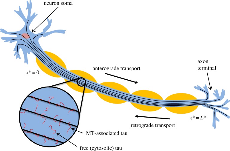
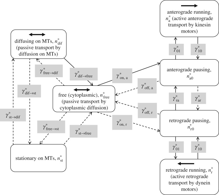
Based on the above reports, we will assume that tau is transported by both active (molecular motors) and passive (diffusion) mechanisms. We hypothesize that at the beginning of the axon the diffusion mechanism may dominate, whereas at large distances from the soma active transport may be the dominant mode of tau transport. Owing to a small diameter to length ratio in axons, tau transport in an axon is assumed to be one dimensional (figure 1). We assume that tau can be in one of seven kinetic states: being transported by molecular motors, anterogradely or retrogradely (the corresponding concentrations are $n_{\mathrm{a}}^{\ast }$ and $n_{\mathrm{r}}^{\ast }$, respectively); pausing on MTs, while still maintaining its connection with anterograde or retrograde motors (the corresponding concentrations are $n_{\mathrm{a}0}^{\ast }$ and $n_{\mathrm{r}0}^{\ast }$, respectively); being freely suspended in the cytoplasm (the corresponding concentration is $n_{\mathrm{free}}^{\ast }$); diffusing along MTs (the corresponding concentration is $n_{\mathrm{dif}}^{\ast }$); and being stationary on MTs (the corresponding concentration is $n_{\mathrm{st}}^{\ast }$). Tau can transition between these kinetic states; the rates of such transitions are characterized by 14 different kinetic constants (figure 2, dashed lines show the transition processes that we later removed in the simplified model).

Figure 1.

A schematic diagram of the problem. A neuron with an axon and a coordinate system in the axon are shown. Tau protein molecules bound to MTs and suspended in the cytosol are also displayed. (Online version in colour.)

Figure 2.

A kinetic diagram used for the development of full and simplified mathematical models. Seven possible kinetic states for tau protein and kinetic processes between these states are displayed. These are the states for which the conservation equations (equations (2.1)–(2.7)) are written. Four of these kinetic states are identical to the kinetic states in a slow axonal transport model for NFs (see fig. 4 of Jung & Brown [29] and fig. 1 of Li et al. [30]). Kinetic processes that are neglected in the simplified model are shown by dashed lines. Kinetic states where tau has mobility are also indicated.

Various versions of tau transport models have been developed in the recent literature. Coupling between transport of tau and fast axonal transport was investigated in [31]. Tau transport models of various complexities, incorporating different numbers of kinetic states (and thus different transport mechanisms) for tau, were developed in [21,32,33]. In this paper, the model suggested in [33] is extended by improving the boundary condition describing tau utilization at the axon terminal. The full model contains 18 parameters whose values cannot be directly determined from published experimental data. The model was simplified by analysing the sensitivity of the model to these parameters. However, even the simplified model contains eight parameters whose values are not readily available in the literature.

Our main goal was then to develop a method to estimate the values of these eight parameters, and their confidence intervals, from indirect experimental data reported in the literature, such as the tau distribution along the axon and average tau transport velocity. The method suggested in [34] for simulating transport of MAP1B protein in axons was further developed and applied to the model of tau transport. The sensitivity of model parameters to noise (discrepancies between model predictions and published experimental data) was estimated by using a bootstrapping approach. First, we estimated the best-fit values of model parameters by minimizing the discrepancy between model predictions and experimental data, which was evaluated by least squares regression (LSR). We then calculated the residuals by subtracting model predictions (for best-fit parameter values) from experimentally measured values. Then, we randomly resampled residuals and generated new, surrogate data by adding the resampled residuals back to the model predictions. The model was fitted with the surrogate ‘experimental’ data, and the new set of model parameters was generated. By repeating this procedure many times, we produced histograms of model parameters, which were used to estimate confidence intervals of the parameters.

2. Material and methods

(a). Full model

The governing equations for tau transport are analogous to those proposed in [33]. We postulate that tau can be transported along the axon by three mechanisms: cytoplasmic diffusion of free tau, diffusion of a sub-population of MT-bound tau along MTs and energy-dependent slow axonal transport driven by kinesin and dynein motors (figure 2). Equations modelling slow axonal transport of tau are based on those developed in [29] for neurofilaments (NFs). We added effects of tau diffusion and degradation (including these two effects was originally proposed in [35,36]). It is assumed that tau participating in slow axonal transport will spend most of the time in a pausing state, while maintaining its association with molecular motors. Only during short periods of mobility does tau move along an MT with ‘fast’ velocity, pulled by kinesin or dynein motors. Recently, an argument was made that pauses in cargo movement can be better explained by motor detachment–reattachment events caused, for example, by a motor reaching the end of an MT or encountering an obstruction [37]. We note that the model developed here is a cargo-level model rather than a motor-level model, and the two ‘pausing’ kinetic states in figure 2 refer to the behaviour of cargo.

Experimental evidence shows that tau can be degraded in axons, primarily through proteolytic degradation [38]. To enter a proteasome's proteolytic chamber (functioning of proteasomes is described, for example, in [39]) tau must be detached from MTs; therefore, we included the degradation term only in the conservation equation for the free tau.

As the proposed model is one dimensional, we characterized tau concentrations in all seven kinetic states (figure 2) by a linear density of tau protein molecules (the number of tau molecules per unit length of the axon). We first stated the conservation of tau in the two kinetic states that are populated by tau molecules that experience short periods of fast motion (when they are pulled by kinesin and dynein motors, respectively). This gives the following equations:

$$\frac{\mathrm{\partial }{n}_{\mathrm{a}}^{\ast }}{\mathrm{\partial }{t}^{\ast }}=-v_{\mathrm{a}}^{\ast }\frac{\mathrm{\partial }{n}_{\mathrm{a}}^{\ast }}{\mathrm{\partial }{x}^{\ast }}-{\gamma }_{10}^{\ast }{n}_{\mathrm{a}}^{\ast }+{\gamma }_{01}^{\ast }{n}_{\mathrm{a}0}^{\ast }$$ 2.1

and

$$\frac{\mathrm{\partial }{n}_{\mathrm{r}}^{\ast }}{\mathrm{\partial }{t}^{\ast }}=v_{\mathrm{r}}^{\ast }\frac{\mathrm{\partial }{n}_{\mathrm{r}}^{\ast }}{\mathrm{\partial }{x}^{\ast }}-{\gamma }_{10}^{\ast }{n}_{\mathrm{r}}^{\ast }+{\gamma }_{01}^{\ast }{n}_{\mathrm{r}0}^{\ast }.$$ 2.2

Asterisks were used to denote dimensional quantities. The terms on the left-hand sides of equations (2.1) and (2.2) describe changes in the concentrations of kinesin-driven and dynein-driven tau. As changes in the axon occur slowly, the problem was solved in a steady-state formulation, and all transient terms in the governing equations were neglected. However, we keep these terms when writing equations of the full model because the proposed model could also be used for solving transient problems. The terms involving the kinesin and dynein motor velocities, $v_{\mathrm{a}}^{\ast }$ and $v_{\mathrm{r}}^{\ast }$, respectively, on the right-hand sides of equations (2.1) and (2.2) describe changes in the concentrations of motor-driven tau due to tau being pulled by the motors. The remaining terms on the right-hand sides of equations (2.1) and (2.2) (the terms with various γ*s) describe the effect of tau transitions to/from the motor-driven states. It should be noted that an individual tau molecule resides in the motor-driven state for only a short time, and motor-driven states should be viewed as dynamic pools populated by tau molecules constantly transitioning between motor-driven and pausing states.

Stating the conservation of tau molecules in the two pausing states gives the following equations:

$$\frac{\mathrm{\partial }{n}_{\mathrm{a}0}^{\ast }}{\mathrm{\partial }{t}^{\ast }}=-({\gamma }_{01}^{\ast }+{\gamma }_{\mathrm{ar}}^{\ast }+{\gamma }_{\mathrm{off},\mathrm{a}}^{\ast })n_{\mathrm{a}0}^{\ast }+{\gamma }_{10}^{\ast }{n}_{\mathrm{a}}^{\ast }+{\gamma }_{\mathrm{ra}}^{\ast }{n}_{\mathrm{r}0}^{\ast }+{\gamma }_{\mathrm{on},\mathrm{a}}^{\ast }{n}_{\mathrm{free}}^{\ast }$$ 2.3

and

$$\frac{\mathrm{\partial }{n}_{\mathrm{r}0}^{\ast }}{\mathrm{\partial }{t}^{\ast }}=-({\gamma }_{01}^{\ast }+{\gamma }_{\mathrm{ra}}^{\ast }+{\gamma }_{\mathrm{off},\mathrm{r}}^{\ast })n_{\mathrm{r}0}^{\ast }+{\gamma }_{10}^{\ast }{n}_{\mathrm{r}}^{\ast }+{\gamma }_{\mathrm{ar}}^{\ast }{n}_{\mathrm{a}0}^{\ast }+{\gamma }_{\mathrm{on},\mathrm{r}}^{\ast }{n}_{\mathrm{free}}^{\ast }.$$ 2.4

The terms on the left-hand sides of equations (2.3) and (2.4) are transient terms, which are neglected in the steady-state formulation. The only terms on the right-hand sides of equations (2.3) and (2.4) are those that describe the transitions between the pausing states and other kinetic states (see the arrows in figure 2). This is because tau molecules have no mobility in the pausing states, and the only way for their concentration to be increased or reduced is through transitioning to/from another kinetic state.

The requirement of conservation of free tau leads to the following equation:

$$\begin{array}{rl}\frac{\mathrm{\partial }{n}_{\mathrm{free}}^{\ast }}{\mathrm{\partial }{t}^{\ast }}& =D_{\mathrm{free}}^{\ast }\frac{{\mathrm{\partial }}^2{n}_{\mathrm{free}}^{\ast }}{\mathrm{\partial }{x^{\ast }}^2}+{\gamma }_{\mathrm{off},\mathrm{a}}^{\ast }{n}_{\mathrm{a}0}^{\ast }+{\gamma }_{\mathrm{off},\mathrm{r}}^{\ast }{n}_{\mathrm{r}0}^{\ast }-({\gamma }_{\mathrm{on},\mathrm{a}}^{\ast }+{\gamma }_{\mathrm{on},\mathrm{r}}^{\ast }+{\gamma }_{\mathrm{free}\to \mathrm{st}}^{\ast }+{\gamma }_{\mathrm{free}\to \mathrm{dif}}^{\ast })n_{\mathrm{free}}^{\ast }\\ & +{\gamma }_{\mathrm{st}\to \mathrm{free}}^{\ast }{n}_{\mathrm{st}}^{\ast }+{\gamma }_{\mathrm{dif}\to \mathrm{free}}^{\ast }{n}_{\mathrm{dif}}^{\ast }-\frac{n_{\mathrm{free}}^{\ast }\ln (2)}{T_{1/2}^{\ast }}.\end{array}$$ 2.5

The term involving the diffusivity of free tau, $D_{\mathrm{free}}^{\ast }$, on the right-hand side of equation (2.5) describes diffusion of tau molecules in the cytoplasm; the last term involving tau's half-life, $T_{1/2}^{\ast }$, describes tau degradation in proteasomes; and the terms on the right-hand side of equation (2.5) involving various γ*s describe tau's transitions to/from the free cytoplasmic state.

The conservation of a sub-population of MT-bound tau that can diffuse along the MTs results in the following equation:

$$\frac{\mathrm{\partial }{n}_{\mathrm{dif}}^{\ast }}{\mathrm{\partial }{t}^{\ast }}=D_{\mathrm{mt}}^{\ast }\frac{{\mathrm{\partial }}^2{n}_{\mathrm{dif}}^{\ast }}{\mathrm{\partial }{x^{\ast }}^2}-({\gamma }_{\mathrm{dif}\to \mathrm{free}}^{\ast }+{\gamma }_{\mathrm{dif}\to \mathrm{st}}^{\ast })n_{\mathrm{dif}}^{\ast }+{\gamma }_{\mathrm{free}\to \mathrm{dif}}^{\ast }{n}_{\mathrm{free}}^{\ast }+{\gamma }_{\mathrm{st}\to \mathrm{dif}}^{\ast }{n}_{\mathrm{st}}^{\ast }.$$ 2.6

The term involving the diffusivity of MT-bound tau, $D_{\mathrm{mt}}^{\ast }$, on the right-hand side of equation (2.6) describes tau diffusion along MTs, a phenomenon that was reported in [25]. The remaining terms on the right-hand side of equation (2.6) describe tau transitions to/from this kinetic state.

The conservation of a sub-population of stationary MT-bound tau leads to the following equation:

$$\frac{\mathrm{\partial }{n}_{\mathrm{st}}^{\ast }}{\mathrm{\partial }{t}^{\ast }}=-({\gamma }_{\mathrm{st}\to \mathrm{free}}^{\ast }+{\gamma }_{\mathrm{st}\to \mathrm{dif}}^{\ast })n_{\mathrm{st}}^{\ast }+{\gamma }_{\mathrm{free}\to \mathrm{st}}^{\ast }{n}_{\mathrm{free}}^{\ast }+{\gamma }_{\mathrm{dif}\to \mathrm{st}}^{\ast }{n}_{\mathrm{dif}}^{\ast }.$$ 2.7

The terms on the right-hand side of equation (2.7) describe transitions of tau protein to/from this kinetic state.

We summarize model variables in table 1 and model parameters in table 2.

Table 1.

A list of model variables.

symbol	definition	unit
$n_{\mathrm{a}}^{\ast }$	concentration of on-track tau moving along MTs anterogradely, propelled by molecular motors	μm−1
$n_{\mathrm{r}}^{\ast }$	concentration of on-track tau moving along MTs retrogradely, propelled by molecular motors	μm−1
$n_{\mathrm{a}0}^{\ast }$	concentration of pausing on-track tau that is still associated with molecular motors and can resume its anterograde motion	μm−1
$n_{\mathrm{r}0}^{\ast }$	concentration of pausing on-track tau that is still associated with molecular motors and can resume its retrograde motion	μm−1
$n_{\mathrm{free}}^{\ast }$	concentration of free (off-track) tau in the cytosol	μm−1
$n_{\mathrm{st}}^{\ast }$	concentration of stationary tau bound to MTs, no association with motors	μm−1
$n_{\mathrm{dif}}^{\ast }$	concentration of tau diffusing along MTs, no association with motors	μm−1
t*a	time	s
x*	Cartesian coordinate along the axon	μm

^aNote that, as the equations are solved for a steady-state situation, time is not involved.

Table 2.

A list of model parameters and their estimated values. Some parameters could be estimated from the literature, other parameters were estimated by minimizing the objective function given by equation (2.18) (see footnote ‘a’ below this table).

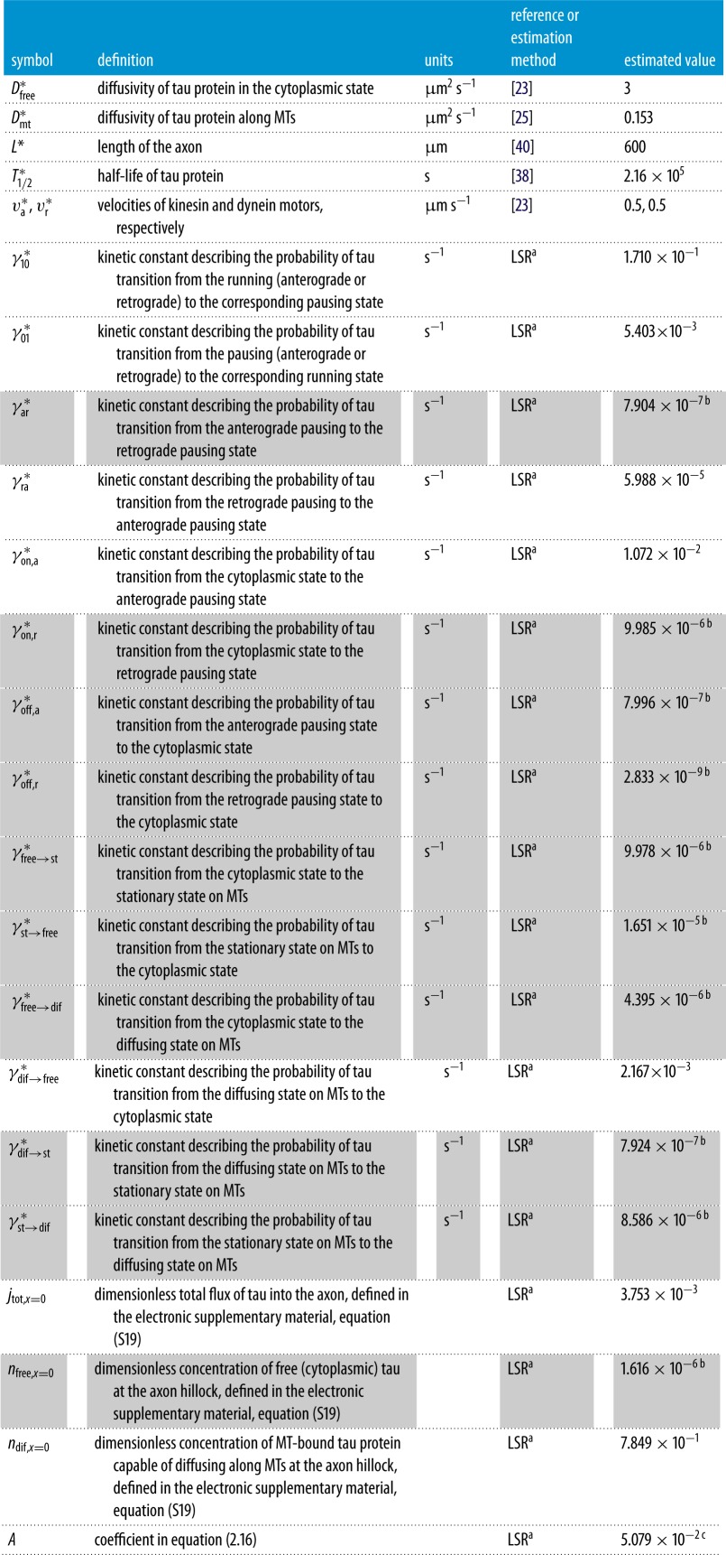^aWe could estimate values of six out of 24 model parameters from the literature. Values of the remaining 18 parameters were estimated by optimizing the agreement between model predictions and published experimental data. The LSR procedure of finding the best-fit parameters is described in §2c(iii).

^bWe investigated and identified which of the 18 parameters whose values were not readily available from the literature affect the solution in a significant way. To do this, we set values of these parameters to zero, one at a time, while leaving all other parameters at their ‘optimal’ values, and checked whether the total tau concentration and the average tau velocity were affected. If the result was the same, we dropped all terms that involved the corresponding parameter from the governing equations. The rows containing parameters that could be dropped are shaded grey.

^cWe also checked whether parameter A can be set to unity. We found that this cannot be done without affecting the solution. As follows from the estimate after equation (2.15), setting parameter A to unity implies a 98.3% chance of tau destruction in the terminal. The optimal value of A given in table 2 implies that only 4.99% of tau is destroyed in the terminal; the rest is reflected back.

Black et al. [40] reported volume density of fluorescence intensity of tau, a quantity that is directly proportional to the total concentration of tau. The total tau concentration can be found by calculating the sum of tau concentrations over all seven kinetic states displayed in figure 2,

$$n_{\mathrm{tot}}^{\ast }=n_{\mathrm{a}}^{\ast }+n_{\mathrm{r}}^{\ast }+n_{\mathrm{a}0}^{\ast }+n_{\mathrm{r}0}^{\ast }+n_{\mathrm{free}}^{\ast }+n_{\mathrm{st}}^{\ast }+n_{\mathrm{dif}}^{\ast }.$$ 2.8

The percentage of tau bound to MTs at a particular location in the axon can be modelled using equation (2.8),

$$\mathrm{\%}\mathrm{bound}=\frac{n_{\mathrm{a}}^{\ast }+n_{\mathrm{r}}^{\ast }+n_{\mathrm{a}0}^{\ast }+n_{\mathrm{r}0}^{\ast }+n_{\mathrm{st}}^{\ast }+n_{\mathrm{dif}}^{\ast }}{n_{\mathrm{tot}}^{\ast }}(100\mathrm{\%}).$$ 2.9

The numerator on the right-hand side of equation (2.9) includes all components of $n_{\mathrm{tot}}^{\ast }$ except $n_{\mathrm{free}}^{\ast }$.

The total flux of tau has contributions only from those kinetic states where tau has some mobility. In general, the total tau flux can be found as

$$j_{\mathrm{tot}}^{\ast }=j_{\mathrm{dif}}^{\ast }+j_{\mathrm{mm}}^{\ast },$$ 2.10

where

$$j_{\mathrm{dif}}^{\ast }=-D_{\mathrm{free}}^{\ast }\frac{\mathrm{\partial }{n}_{\mathrm{free}}^{\ast }}{\mathrm{\partial }{x}^{\ast }}-D_{\mathrm{mt}}^{\ast }\frac{\mathrm{\partial }{n}_{\mathrm{dif}}^{\ast }}{\mathrm{\partial }{x}^{\ast }}$$ 2.11

is the diffusion-driven flux of tau and

$$j_{\mathrm{mm}}^{\ast }=v_{\mathrm{a}}^{\ast }{n}_{\mathrm{a}}^{\ast }-v_{\mathrm{r}}^{\ast }{n}_{\mathrm{r}}^{\ast }$$ 2.12

is the molecular motor-driven flux of tau.

The average velocity of tau protein, a quantity that depends on x*, can be calculated as follows:

$$v_{\mathrm{av}}^{\ast }=\frac{j_{\mathrm{tot}}^{\ast }}{n_{\mathrm{tot}}^{\ast }}.$$ 2.13

(b). Boundary conditions

At the axon hillock, we imposed the following boundary conditions:

$$\mathrm{at}\hspace{0.17em}{x}^{\ast }=0:n_{\mathrm{free}}^{\ast }=n_{\mathrm{free},x=0}^{\ast },j_{\mathrm{tot}}^{\ast }=j_{\mathrm{tot},x=0}^{\ast }\mathrm{and}{n}_{\mathrm{dif}}^{\ast }=n_{\mathrm{dif},x=0}^{\ast }.$$ (2.14a,b,c)

The parameter $j_{\mathrm{tot},x=0}^{\ast }$ represents the rate at which tau enters the axon. As we analyse the neuron at steady-state conditions, $j_{\mathrm{tot},x=0}^{\ast }$ is equal to the rate of tau production in the soma. None of the parameters $n_{\mathrm{free},x=0}^{\ast }$, $j_{\mathrm{tot},x=0}^{\ast }$ and $n_{\mathrm{dif},x=0}^{\ast }$ are available from the literature, thus we determined the values of these parameters by fitting model predictions with published experimental data. Note that we used dimensionless values of these parameters in the numerical implementation; these are defined in the electronic supplementary material, equation (S19).

We experimented with different forms of boundary conditions at the axon terminal (for example, we tried imposing some arbitrary values for $n_{\mathrm{free},x=L}^{\ast }$ and $n_{\mathrm{dif},x=L}^{\ast }$ and adjusted these values by fitting model predictions with published experimental data). We found that the best agreement in terms of the shape of the total tau concentration (equation (2.8)) was achieved by postulating zero gradients of $n_{\mathrm{free},x=L}^{\ast }$ and $n_{\mathrm{dif},x=L}^{\ast }$ at the terminal. In terms of the tau flux at the terminal, some published data suggest that tau is required for synapse maintenance [41]. We, therefore, assumed that a portion of tau that reaches the terminal eventually degrades at the terminal; the rest is reflected back. These assumptions result in the following boundary conditions at the terminal:

$$\mathrm{at}\hspace{0.17em}{x}^{\ast }=L^{\ast }:\frac{\mathrm{\partial }{n}_{\mathrm{free}}^{\ast }}{\mathrm{\partial }{x}^{\ast }}=0,j_{\mathrm{tot}}^{\ast }=j_{\mathrm{tot},x=L}^{\ast }\mathrm{and}\frac{\mathrm{\partial }{n}_{\mathrm{dif}}^{\ast }}{\mathrm{\partial }{x}^{\ast }}=0.$$ (2.15a,b,c)

We rewrite equation (2.15b) in a more detailed form by using the approach developed in [30] for NFs. Tau that enters the terminal can either reverse and leave the terminal or be degraded; the probability of its degradation is estimated as $1-\exp [-{\gamma }_{\mathrm{deg}}^{\ast }{t}_{\mathrm{rev}}^{\ast }]$. Here, ${\gamma }_{\mathrm{deg}}^{\ast }$ is a kinetic constant characterizing tau degradation (estimated as $\ln (2)/T_{1/2}^{\ast }$) and $t_{\mathrm{rev}}^{\ast }$ is the time required for a motor-driven tau protein to reverse its direction at the terminal (estimated as $1/{\gamma }_{\mathrm{ar}}^{\ast }$). Using the values for parameters $T_{1/2}^{\ast }$ and ${\gamma }_{\mathrm{ar}}^{\ast }$ that are given in table 2, the probability of tau degradation at the terminal is 98.3%. Such a high probability of tau degradation can be explained by the small value of ${\gamma }_{\mathrm{ar}}^{\ast }$, which indicates that it takes a large length of time for tau to change an anterograde motor to a retrograde motor. The remaining tau (1.7%) may reverse its direction and leave the terminal. However, this estimate may be inaccurate because the exchange of motors in the terminal may occur much faster than during tau transit in the axon. To provide the model with more flexibility, we multiplied this estimate by parameter A, whose value is determined by fitting model predictions with published experimental data. The introduction of parameter A is an extension of our previous model of tau transport reported in [33]. This gives the following expanded form of equation (2.15b):

$$-D_{\mathrm{free}}^{\ast }\frac{\mathrm{\partial }{n}_{\mathrm{free}}^{\ast }}{\mathrm{\partial }{x}^{\ast }}-D_{\mathrm{mt}}^{\ast }\frac{\mathrm{\partial }{n}_{\mathrm{dif}}^{\ast }}{\mathrm{\partial }{x}^{\ast }}+v_{\mathrm{a}}^{\ast }{n}_{\mathrm{a}}^{\ast }-v_{\mathrm{r}}^{\ast }{n}_{\mathrm{r}}^{\ast }=A\left(1-\exp \left[-\frac{\ln (2)}{T_{1/2}^{\ast }}\frac{1}{{\gamma }_{\mathrm{ar}}^{\ast }}\right]\right)v_{\mathrm{a}}^{\ast }{n}_{\mathrm{a}}^{\ast }.$$ 2.16

Here, we used equations (2.10)–(2.12) to represent the total tau flux on the left-hand side of equation (2.15b), and we also assumed that tau enters the terminal being pulled by anterograde motors, which estimates its flux into the terminal as $v_{\mathrm{a}}^{\ast }{n}_{\mathrm{a}}^{\ast }$.

(c). Numerical procedures

(i). Numerical solution of differential equations

Equations (2.1)–(2.7) were solved for steady-state conditions in the axon. The results are also applicable to slowly growing axons, providing that their growth is sufficiently slow so that tau concentrations effectively relax to their steady-state distributions. Equations (2.3), (2.4) and (2.7) then become algebraic equations, and we used these equations to eliminate $n_{\mathrm{a}0}^{\ast }(x)$, $n_{\mathrm{r}0}^{\ast }(x)$ and $n_{\mathrm{st}}^{\ast }(x)$ from the remaining equations. As a result of this substitution, four ordinary differential equations for $n_{\mathrm{a}}^{\ast }(x)$, $n_{\mathrm{r}}^{\ast }(x)$, $n_{\mathrm{free}}^{\ast }(x)$ and $n_{\mathrm{dif}}^{\ast }(x)$ were obtained, which were solved using Matlab's BVP4C solver (Matlab R2016a; MathWorks, Natick, MA, USA). We used the default settings of the BVP4C solver (we checked that the solution was not affected when we reduced the values of error tolerance parameters, RelTol and AbsTol). After that, we computed $n_{\mathrm{a}0}^{\ast }(x)$, $n_{\mathrm{r}0}^{\ast }(x)$ and $n_{\mathrm{st}}^{\ast }(x)$ by using equations (2.3), (2.4) and (2.7).

(ii). Digitizing experimental data for the tau concentration

By using GetData Graph Digitizer, we scanned 55 points representing the experimentally measured tau concentration reported in fig. 7D of Black et al. [40] for a 600 µm long axon. We only scanned those points that were between 0 and 600 µm away from the soma. Black et al. [40] also reported tau concentrations at a few points for x* > 600 µm (the points that are within the synapse), but, as our model does not simulate biochemistry occurring in the synapse, we did not scan these points. Black et al. [40] used arbitrary units when they reported fluorescence intensity of tau per unit volume of the axon in fig. 7D. In accordance with the definition of the dimensionless tau concentration in the electronic supplementary material, equation (S1), we assigned a value of 1 to this quantity in the left-most point in fig. 7D (corresponding to x* = 0). This means that we effectively rescaled the total tau concentration as

$$n_{\mathrm{tot}}=\frac{n_{\mathrm{tot}}^{\ast }}{n_{\mathrm{tot},x=0}^{\ast }}.$$ 2.17

(iii). Finding the parameter set that gives the best fit with experimental results

Estimating model parameters is an inverse problem [42,43]. The solution to this problem can be found by performing nonlinear optimization and finding the set of parameters that minimizes an appropriately defined objective (penalty) function which evaluates the discrepancies between model predictions and experimental measurements. This approach was used in [44,45] to determine the parameters in a model simulating flow in unsaturated soils, which is described by the Richards equation [46]. This approach was also utilized in [47] to estimate parameters for a model of fast axonal transport, which was developed in [48]. This approach was further used in [49] to estimate parameters for a model simulating the dynamics of biomolecules in living organisms.

In our problem, we have different types of published data. To solve the inverse problem, we used multi-objective optimization [50]. We used the following weighted objective function which combines three different effects:

$$\begin{array}{r}err=\sum _{i=1}^N{(n_{\mathrm{tot},i}-n_{\mathrm{tot},\mathrm{exper},i})}^2+{\omega }_1\sum _{i=1}^N{(v_{\mathrm{a}v,i}^{\ast }-0.00345\hspace{0.17em}\mu \mathrm{m}\hspace{0.17em}{\mathrm{s}}^{-1})}^2+{\omega }_2{({\mathrm{\%}\mathrm{bound}|}_{x=L/2}-100)}^2,\end{array}$$ 2.18

where N = 55 represents the number of data points that we obtained by scanning tau concentration data reported in [40]. The deviations between model predictions and experimental data were estimated by LSR [42]. The first term on the right-hand side of equation (2.18) characterizes the deviation between predicted and experimentally measured tau concentrations, the second term characterizes the deviation of the predicted tau velocity from 0.00345 µm s⁻¹ (the average of the range of tau velocity reported in [51]), and the third term ensures that in the centre of the axon most tau is bound to MTs. Because experimental data for the tau concentration are reported in [40] in arbitrary units, and hence we had to rescale this dataset when digitizing it, the first term on the right-hand side of equation (2.18) involves dimensionless total tau concentrations, defined in equation (2.17).

The weighting factors ω₁ and ω₂ in equation (2.18) were set to 10 000 s² µm⁻² and 1, respectively, to provide good visual agreement with experimental data. These values were selected after extensive experimentation with the weighting factors. The large value of ω₁ is explained by a small value of the average tau velocity; ω₁ has to be large for the second term to be a contributor to the objective function. If the weighting factor ω₁ is decreased, then the agreement between the experimentally measured tau concentration and its model prediction is improved, but the agreement in terms of the average tau velocity gets worse (in the electronic supplementary material, figure S1 compares cases with ω₁ = 10 000 s² µm⁻² and 1).

To find the global minimum of the objective function, we used MultiStart with a local solver fmincon; these routines are included in Matlab's Optimization Toolbox. fmincon requires a starting point to be specified, which is used to initiate a descent to a minimum. To increase the likelihood of finding a global minimum, we used MultiStart with 100 000 randomly selected starting points for the full model and with 10 000 randomly selected starting points for the simplified model. We used a Dell Precision T7810 Workstation with an Intel Xeon 2.40 GHz processor (hereafter Dell Workstation) to perform computations. The computational time was 182 h for the full model and 12 h for the simplified model (see §2c(iv)). Sixteen workers were used for each computation reported in this paper.

(iv). Simplified model, steady-state formulation

We attempted to simplify the full model by identifying parameters that can be dropped from the governing equation without affecting the solution. We performed computations by going through all 18 parameters, setting them to zero, one by one and comparing the resulting solution with the solution of the full model. We found that we can drop 10 parameters, and all the terms containing these parameters, from the equations of the full model without affecting the solution to a significant degree (figures 3 and 4; electronic supplementary material, figures S2–S5). The parameters that we dropped were ${\gamma }_{\mathrm{ar}}^{\ast }$, ${\gamma }_{\mathrm{on},\mathrm{r}}^{\ast }$, ${\gamma }_{\mathrm{off},\mathrm{a}}^{\ast }$, ${\gamma }_{\mathrm{off},\mathrm{r}}^{\ast }$, ${\gamma }_{\mathrm{free}\to \mathrm{st}}^{\ast }$, ${\gamma }_{\mathrm{st}\to \mathrm{free}}^{\ast }$, ${\gamma }_{\mathrm{free}\to \mathrm{dif}}^{\ast }$, ${\gamma }_{\mathrm{dif}\to \mathrm{st}}^{\ast }$, ${\gamma }_{\mathrm{st}\to \mathrm{dif}}^{\ast }$ and $n_{\mathrm{free},x=0}^{\ast }$. The rows containing these parameters are shaded grey in table 2. We also showed kinetic processes that we eliminated from the full model by using dashed lines in figure 2. As the problem was solved for a steady-state case, below we give equations for the simplified model in a steady-state formulation. The equations for the motor-driven tau, pulled along MTs (anterogradely and retrogradely, respectively), are

$$-v_{\mathrm{a}}^{\ast }\frac{\mathrm{d}{n}_a^{\ast }}{\mathrm{d}{x}^{\ast }}-{\gamma }_{10}^{\ast }{n}_{\mathrm{a}}^{\ast }+{\gamma }_{01}^{\ast }{n}_{\mathrm{a}0}^{\ast }=0$$ 2.19

and

$$v_{\mathrm{r}}^{\ast }\frac{\mathrm{d}{n}_{\mathrm{r}}^{\ast }}{\mathrm{d}{x}^{\ast }}-{\gamma }_{10}^{\ast }{n}_{\mathrm{r}}^{\ast }+{\gamma }_{01}^{\ast }{n}_{\mathrm{r}0}^{\ast }=0.$$ 2.20

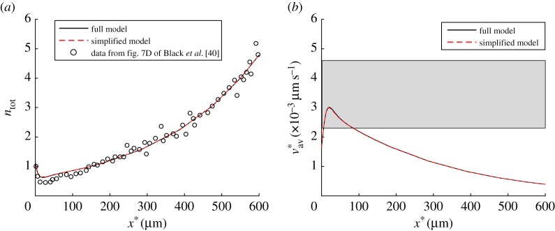
Figure 3.

(a) Dimensionless total concentration of tau versus position in the axon. Open circles show experimental data from fig. 7D of Black et al. [40]. As fig. 7D of Black et al. [40] shows tau concentrations in arbitrary units, we rescaled data from this figure such that the experimentally measured tau concentration in the most leftward point (at x = 0) was equal to 1. (b) Tau average velocity versus position in the axon. A horizontal band shows the range of the average velocity of tau protein reported in [51] (ω₁= 10 000 s² µm⁻², ω₂ = 1.) (Online version in colour.)

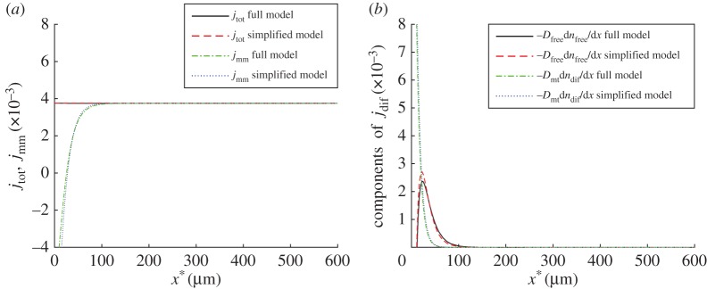
Figure 4.

(a) Total dimensionless tau flux and molecular motor-driven tau flux versus position in the axon. (b) Two components of the dimensionless diffusion-driven tau flux, due to diffusion of cytoplasmic tau, $-D_{\mathrm{free}}(\mathrm{d}{n}_{\mathrm{free}}/\mathrm{d}x)$, and due to diffusion of MT-bound tau, $-D_{\mathrm{mt}}(\mathrm{d}{n}_{\mathrm{dif}}/\mathrm{d}x)$, versus position in the axon (ω₁= 10 000 s² µm⁻², ω₂= 1 ). (Online version in colour.)

The equations for tau concentrations in the pausing states (anterograde and retrograde, respectively) are

$$-{\gamma }_{01}^{\ast }{n}_{\mathrm{a}0}^{\ast }+{\gamma }_{10}^{\ast }{n}_{\mathrm{a}}^{\ast }+{\gamma }_{\mathrm{ra}}^{\ast }{n}_{\mathrm{r}0}^{\ast }+{\gamma }_{\mathrm{on},\mathrm{a}}^{\ast }{n}_{\mathrm{free}}^{\ast }=0$$ 2.21

and

$$-({\gamma }_{01}^{\ast }+{\gamma }_{\mathrm{ra}}^{\ast })n_{\mathrm{r}0}^{\ast }+{\gamma }_{10}^{\ast }{n}_{\mathrm{r}}^{\ast }=0.$$ 2.22

The equation for the concentration of free tau is

$$D_{\mathrm{free}}^{\ast }\frac{{\mathrm{d}}^2{n}_{\mathrm{free}}^{\ast }}{\mathrm{d}{x^{\ast }}^2}-{\gamma }_{\mathrm{on},\mathrm{a}}^{\ast }{n}_{\mathrm{free}}^{\ast }+{\gamma }_{\mathrm{dif}\to \mathrm{free}}^{\ast }{n}_{\mathrm{dif}}^{\ast }-\frac{n_{\mathrm{free}}^{\ast }\ln (2)}{T_{1/2}^{\ast }}=0.$$ 2.23

Equation (2.23) can be solved subject to boundary conditions (2.14a) and (2.15a). The result is given in the electronic supplementary material, equation (S32).

The equation for the stationary population of tau on MTs is

$$n_{\mathrm{st}}^{\ast }=0.$$ 2.24

Owing to equation (2.24), the parameter ${\gamma }_{\mathrm{st}\to \mathrm{free}}^{\ast }$ drops out from the simplified model.

The equation for the population of tau that diffuses along MTs is

$$D_{\mathrm{mt}}^{\ast }\frac{{\mathrm{d}}^2{n}_{\mathrm{dif}}^{\ast }}{\mathrm{d}{x^{\ast }}^2}-{\gamma }_{\mathrm{dif}\to \mathrm{free}}^{\ast }{n}_{\mathrm{dif}}^{\ast }=0.$$ 2.25

Equation (2.25) can be solved subject to boundary conditions (2.14c) and (2.15c). The result is given in the electronic supplementary material, equation (S33).

Boundary conditions given by equations (2.14) and (2.15) stand; as in the simplified model ${\gamma }_{\mathrm{ar}}^{\ast }\to 0$, equation (2.16) can be now simplified as

$$-D_{\mathrm{free}}^{\ast }\frac{\mathrm{\partial }{n}_{\mathrm{free}}^{\ast }}{\mathrm{\partial }{x}^{\ast }}-D_{\mathrm{mt}}^{\ast }\frac{\mathrm{\partial }{n}_{\mathrm{dif}}^{\ast }}{\mathrm{\partial }{x}^{\ast }}+v_{\mathrm{a}}^{\ast }{n}_{\mathrm{a}}^{\ast }-v_{\mathrm{r}}^{\ast }{n}_{\mathrm{r}}^{\ast }=A{v}_{\mathrm{a}}^{\ast }{n}_{\mathrm{a}}^{\ast }.$$ 2.26

(v). Resampling residuals in order to generate histograms of best-fit parameters and establish their confidence intervals

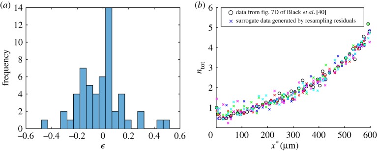
We used resampling residuals, which is a type of bootstrapping technique [52,53], in order to characterize the dependency of best-fit values of model parameters on experimental data inputs. The first step was finding residuals, which were defined as differences between experimentally determined values of the total tau concentration and model predictions of the same quantity. The number of residuals was equal to the number of experimental measurements (in our case, N = 55):

$${\epsilon }_i=n_{\mathrm{tot},\mathrm{exper},i}-n_{\mathrm{tot},i}(i=1,\dots ,N).$$ 2.27

We then generated M sets of new, surrogate data by randomly resampling residuals and adding them back to experimental values,

$${\hat{n}}_{\mathrm{tot},\mathrm{exper},i}=n_{\mathrm{tot},i}+{\epsilon }_j,$$ 2.28

where j was randomly drawn, with replacement, from the list (1, … ,N). We thus assumed that the residuals, which we defined as the deviation between the experimental data and model predictions, are characterized by an underlying distribution which is independent of position in the axon. (This implies that the histogram displayed in figure 5a is the result of sampling from this underlying distribution.) Using equation (2.28) 5000 times (M = 5000) allowed us to obtain 5000 sets of surrogate data for the total tau concentration. Applying the procedure of finding the best-fit parameters (described in §2c(iii)) to these surrogate datasets allowed us to produce 5000 new sets of best-fit parameters, which were used to produce histograms of parameters for each of the eight parameters of the simplified model.

Figure 5.

(a) Histogram showing the frequency of 55 residuals which are defined by equation (2.27); the residuals show the difference between the true experimental data reported in fig. 7D of Black et al. [40] and model predictions for the total tau concentration, computed for the best-fit parameter set. (b) The actual experimental data for the total tau concentration are shown by open circles. Five randomly selected surrogate datasets (out of 5000 surrogate datasets used to produce the histograms) are shown by crosses. (Online version in colour.)

We then used these histograms to determine the confidence intervals of parameters. This was done using the percentile bootstrap. We found 90% confidence intervals for each parameter by using Matlab's prctile function, which effectively trims 5% from the lower and upper ends of the corresponding histogram. The percentile bootstrap was selected because the best-fit procedure described in §2c(iii) always produces positive parameter values and, therefore, the confidence intervals produced by the percentile bootstrap also have positive boundaries. This is advantageous because on physical grounds the model parameters cannot be negative. The limitation of the percentile bootstrap is the assumption that the sampling distribution provides a good approximation for the population distribution [54,55]; see also K Singh, M Xie 2008 Bootstrap: a statistical method (http://stat.rutgers.edu/home/mxie/RCPapers/bootstrap.pdf). The developed method is also based on the assumption that the distribution of residuals is independent of x. This assumption needs further validation.

3. Results

(a). Best-fit parameter values for the full model obtained by minimizing the objective function

We obtained best-fit parameter values for the full model by minimizing the objective function given by equation (2.18), as described in §2c(iii). The best-fit values are given in column 5 of table 2. We used 100 000 randomly selected starting points for the MultiStart routine, each of which was used to initiate a multi-parametric minimization. The computational time on the Dell Workstation was 182 h. The obtained minimum value of the objective function was 3.271464. To ensure that the result was independent of the number of starting points, we decreased the number of random starting points to 50 000, and obtained the same result.

(b). Best-fit parameter values for the simplified model obtained by minimizing the objective function

Values of parameters $D_{\mathrm{dif}}^{\ast }$, $D_{\mathrm{mt}}^{\ast }$, L*, $T_{1/2}^{\ast }$, $v_{\mathrm{a}}^{\ast }$ and $v_{\mathrm{r}}^{\ast }$ (the first five rows in table 2) are the same for the full and simplified models. Values of the other eight parameters in the simplified model were found by minimizing the objective function defined by equation (2.18), following the procedure described in §2c(iii). We then used 10 000 random points to start the minimization procedure. Computations took 12 h on the Dell Workstation; the obtained minimum value of the objective function was 3.271769, which, as expected, was slightly larger than for the full model. We checked the convergence of the results by rerunning minimization with a reduced number (5000) of random starting points. The same best-fit values of model parameters were obtained. As the full and simplified models contain different numbers of parameters, the best-fit values of the eight parameters of the simplified model are not the same as the values of the corresponding parameters in the full model (cf. the corresponding rows in tables 2 and 3). This indicates that some of the parameters are interdependent. Despite such interdependencies, the best-fit values for the full model fall within 90% confidence intervals for parameters of the simplified model (column 4 of table 3). The only exception is ${\gamma }_{\mathrm{on},\mathrm{a}}^{\ast }$; this exception is explained in footnote ‘c’ in table 3.

Table 3.

Parameters of the simplified model determined by minimizing the objective function given by equation (2.18) and their confidence intervals found by resampling residuals.

symbol	units	estimated value by LSRa	(90% CI)b
${\gamma }_{10}^{\ast }$	s−1	9.778 × 10−2	(8.70 × 10−2, 8.84 × 10−1)
${\gamma }_{01}^{\ast }$	s−1	3.032 × 10−3	(2.08 × 10−3, 2.81 × 10−2)
${\gamma }_{\mathrm{ra}}^{\ast }$	s−1	5.850 × 10−5	(2.72 × 10−5, 7.60 × 10−5)
${\gamma }_{\mathrm{on},\mathrm{a}}^{\ast }$	s−1	1.496 × 10−2 c	(3.40 × 10−2, 6.48 × 100)
${\gamma }_{\mathrm{dif}\to \mathrm{free}}^{\ast }$	s−1	2.139 × 10−3	(1.02 × 10−4, 3.56 × 10−2)
$j_{\mathrm{tot},x=0}$		3.760 × 10−3 d	(3.73 × 10−3, 4.22 × 10−3)
$n_{\mathrm{dif},x=0}$		9.274 × 10−1	(4.44 × 10−1, 3.52 × 100)
A		5.088 × 10−2	(4.02 × 10−2, 1.23 × 10−1)

^aThe same nonlinear optimization procedure that was used for the full model was used for the simplified model. The description of this procedure is given in §2c(iii).

^bWe used 5000 bootstrap resamples to obtain histograms of eight unknown parameters of the simplified model. Computations on the Dell Workstation using 16 workers took 195 h. Once the histograms were obtained, we computed confidence intervals for the eight parameters utilizing the percentile bootstrap, as described in §2c(v).

^cThe histogram for parameter ${\gamma }_{\mathrm{on},\mathrm{a}}^{\ast }$ is heavily skewed to the right (see §3d). For this case, the best-fit value of ${\gamma }_{\mathrm{on},\mathrm{a}}^{\ast }$, given in the third column of table 3, is less than the lowermost value of the confidence interval for this parameter. This simply shows that some results (in this case, the best-fit parameter obtained for the actual experimental data) can fall outside the 90% confidence interval.

^dIt is interesting that the best-fit value of parameter $j_{\mathrm{tot},x=0}$ is displaced to the left portion of the histogram, rather than being in the centre (see §3d). This means that variations in the input data are more likely to cause an increase in tau flux into the axon rather than a decrease. This may suggest that the actual tau distribution in the axon, reported in [40], is optimized as a result of evolution such that the tau utilization in the axon is minimized. This is consistent with the idea expressed in [56] that the highest concentration of tau closest to the synapse is due to optimization of tau's function within the axon.

(c). Comparison between solutions of the full and simplified models

The total tau concentration and the average tau velocity predicted by the full model are almost identical to distributions of the same quantities predicted by the simplified model (figure 3a,b). The fact that the full and simplified models give very close results is further demonstrated by comparing specific components of the total tau concentration and the percentage of MT-bound tau; these comparisons are shown in the electronic supplementary material, figures S2–S5.

As the problem is solved in a steady-state formulation, the total (diffusion-driven plus motor-driven) flux of tau, j_tot, must be independent of x* unless there is some destruction of tau in the axon. In our model, tau can be destroyed (the last term in equation (2.5)), but only in the cytoplasmic state. As the concentration of tau in the cytoplasmic state is very small (electronic supplementary material, figures S4a and S5b), there is little tau destruction in the axon and j_tot remains almost constant (figure 4a).

The motor-driven component is the main component of tau flux in most of the axon (figure 4a), except in a 100 μm long segment next to the soma, where the diffusion-driven flux is a significant contributor to overall tau transport (figure 4b). There are two components of the diffusion-driven flux, one due to diffusion of cytoplasmic tau and the other due to diffusion of a sub-population of MT-bound tau. It is interesting that diffusion of MT-bound tau is effective for tau transport only within the first 50 µm of the axon length while diffusion of cytoplasmic tau can transport tau for the first 100 µm of the axon length (figure 4b). This is because diffusivity of cytoplasmic tau is approximately 20 times larger than diffusivity of MT-bound tau (table 2). Another interesting observation is that tau seems to be driven into the axon mostly by diffusion (figure 4b). This finding explains the dip in the tau concentration at the beginning of the axon, which can be observed in the tau distribution reported in [40] (figure 3a). Once motor-driven transport overpowers diffusion, the total tau concentration increases continuously along the axon until the terminal (figure 3a).

The average tau velocity is calculated as the total tau flux over the total tau concentration (equation (2.13)). As the total flux of tau is almost independent of x* (figure 4a), the average tau velocity is the inverse of n_tot. This inverse relationship explains why $v_{\mathrm{av}}^{\ast }$ first increases (as n_tot decreases) and then decreases (as n_tot increases) (figure 3b).

(d). Confidence intervals of the best-fit parameter values for the simplified model

Best-fit parameter values provide point estimates. For these estimates to be meaningful, confidence intervals for the best-fit parameter values should also be reported. To estimate confidence intervals, one needs many sets of experimental data. To overcome the difficulty of having a very limited amount of published experimental data, we propose to use bootstrapping. Our method is described in §2c(v); the idea is to calculate the residuals between the experimental measurements (open circles in figure 3a) and model predictions (points taken from the solid line in figure 3a for the same values of x* at which experimental measurements were taken; see equation (2.27)). Bootstrapping does not require the residuals to be normally distributed (figure 5a). We then generated a large amount of surrogate ‘experimental’ data by randomly resampling residuals and adding them back to the model predictions (equation (2.28)). Five randomly selected sets of surrogate data for the total tau concentration (out of 5000 used to produce the histograms of model parameters) are shown by crosses in figure 5b. In the electronic supplementary material, figures S6–S11, we show by dashed lines the solutions of the simplified model with parameters determined such that the objective function was minimized for one particular surrogate dataset (tau concentrations for this surrogate dataset are shown by crosses in the electronic supplementary material, figure S10a). Solid lines in figures S6--S11 in the electronic supplementary material display, for comparison, solutions with parameters determined such that the objective function was minimized for the actual experimental data (before any resampling, see open circles in the electronic supplementary material, figure S10a).

By finding best-fit parameter values for the surrogate datasets, we generated histograms for all eight parameters of the simplified model. As the model was fitted with a new dataset each time, the minimized value of the objective function (equation (2.18)) for each surrogate dataset was different. The similarity between the histogram of minimized values of the objective function and a normal distribution is noteworthy (figure 6).

Figure 6.

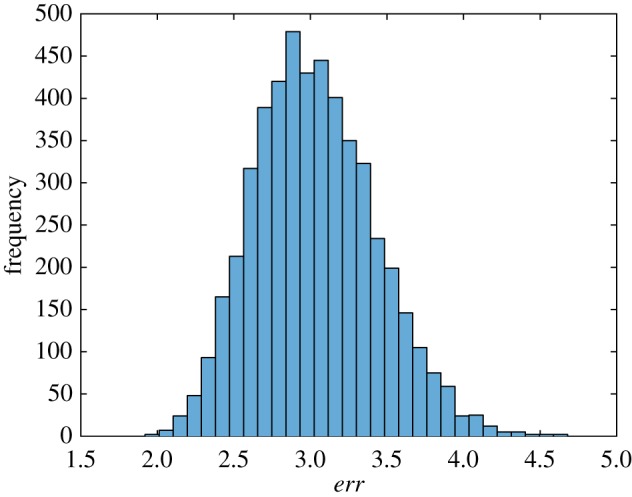
Histogram showing frequency of the minimized value of the objective function, err, defined by equation (2.18), for different bootstrap realizations in each interval denoted with a bar (ω₁= 10 000 s² µm⁻², ω₂= 1). (Online version in colour.)

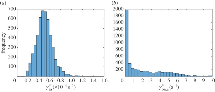
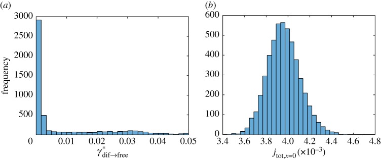
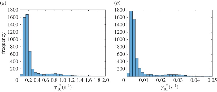
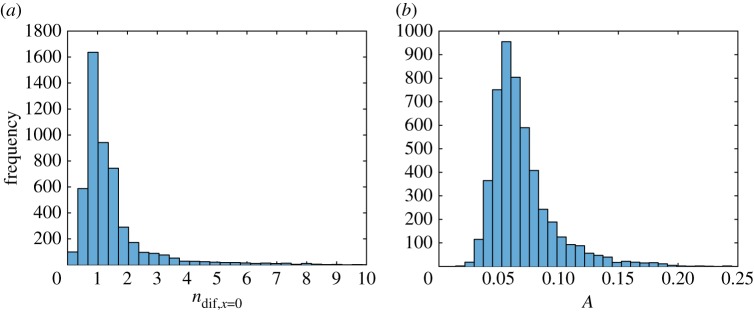
Out of eight parameters of the simplified model, only two, ${\gamma }_{\mathrm{ra}}^{\ast }$ (figure 7a) and $j_{\mathrm{tot},x=0}$ (figure 8b), have histograms that are close to a normal distribution. Histograms of six other parameters, ${\gamma }_{\mathrm{on},\mathrm{a}}^{\ast }$, ${\gamma }_{\mathrm{dif}\to \mathrm{free}}^{\ast }$, ${\gamma }_{10}^{\ast }$, ${\gamma }_{01}^{\ast }$, $n_{\mathrm{dif},x=0}$ and A, are skewed to the right (figures 7b, 8a, 9a,b and 10a,b). Histograms of four out of these six parameters, ${\gamma }_{10}^{\ast }$ (figure 9a), ${\gamma }_{01}^{\ast }$ (figure 9b), ${\gamma }_{\mathrm{on},\mathrm{a}}^{\ast }$ (figure 7b) and ${\gamma }_{\mathrm{dif}\to \mathrm{free}}^{\ast }$ (figure 8a), show a small secondary peak, which makes the histograms bimodal. Parameters ${\gamma }_{01}^{\ast }$, ${\gamma }_{\mathrm{on},\mathrm{a}}^{\ast }$, $n_{\mathrm{dif},x=0}$ and A have the widest 90% confidence intervals while parameters ${\gamma }_{\mathrm{ra}}^{\ast }$ and $j_{\mathrm{tot},x=0}$ have the most narrow 90% confidence intervals (column 4 of table 3). To ensure that using 5000 bootstrap samples gave us converged results, we recomputed histograms and confidence intervals of model parameters with a smaller number (2500) of surrogate datasets; no significant difference was found.

Figure 7.

Histogram showing frequency of parameters (a) ${\gamma }_{\mathrm{ra}}^{\ast }$ and (b) ${\gamma }_{\mathrm{on},\mathrm{a}}^{\ast }$ for different bootstrap realizations in each interval denoted with a bar (ω₁= 10 000 s² µm⁻², ω₂= 1). (Online version in colour.)

Figure 8.

Histogram showing frequency of parameters (a) ${\gamma }_{\mathrm{dif}\to \mathrm{free}}^{\ast }$ and (b) $j_{\mathrm{tot},x=0}$ for different bootstrap realizations in each interval denoted with a bar (ω₁= 10 000 s² µm⁻², ω₂= 1). (Online version in colour.)

Figure 9.

Histogram showing frequency of parameters (a) ${\gamma }_{10}^{\ast }$ and (b) ${\gamma }_{01}^{\ast }$ for different bootstrap realizations in each interval denoted with a bar (ω₁= 10 000 s² µm⁻² ω₂= 1). (Online version in colour.)

Figure 10.

Histogram showing frequency of parameters (a) $n_{\mathrm{dif},x=0}$ and (b) A for different bootstrap realizations in each interval denoted with a bar (ω₁= 10 000 s² µm⁻², ω₂= 1). (Online version in colour.)

4. Discussion of the results, limitations of this study and future directions

We minimized the number of parameters involved in our model, calibrated the model by fitting it with published experimental data and analysed the sensitivity of best-fit parameters to the input data. By randomly resampling residuals and fitting the model into the obtained surrogate data, we produced histograms of model parameters and determined confidence intervals of the parameters. For many parameters (e.g. for ${\gamma }_{01}^{\ast }$, ${\gamma }_{\mathrm{on},\mathrm{a}}^{\ast }$, $n_{\mathrm{dif},x=0}$ and A) confidence intervals are wide. This simply means that published experimental data are not sufficient to determine the values of these parameters with a high accuracy. On the other hand, a value of parameter $j_{\mathrm{tot},x=0}$ can be determined quite accurately. This is an important parameter because it gives the rate of tau synthesis in the soma, and our results suggest that published experimental data are sufficient to accurately estimate this parameter. Another parameter with a narrow confidence interval is ${\gamma }_{\mathrm{ra}}^{\ast }$; this parameter characterizes the probability for tau to lose its connection with retrograde motors and connect to anterograde motors.

Histograms of parameters ${\gamma }_{10}^{\ast }$, ${\gamma }_{01}^{\ast }$, ${\gamma }_{\mathrm{on},\mathrm{a}}^{\ast }$ and ${\gamma }_{\mathrm{dif}\to \mathrm{free}}^{\ast }$ are bimodal; they show small secondary peaks. This means that a small perturbation in an experimental value, for example in a measured value of tau concentration along the axon, may lead to a significant shift in a parameter value, a behaviour resembling a bifurcation.

Some interesting biological conclusions can be drawn from the finding that 10 of 18 parameters can be dropped from the full model in order to create a simplified model, which gives results that are almost identical to those given by the full model (figures 3 and 4; electronic supplementary material, figures S2–S5). In particular, in the simplified model all MT-bound tau is either motor-driven, pausing or diffusing along MTs. There is no stationary tau on MTs; all tau that is attached to MTs either participates in slow axonal transport or diffuses along MTs. The concentration of cytoplasmic tau is generally small, although some amount of cytoplasmic tau is present at the beginning of the axon (electronic supplementary material, figure S4a).

We then used the calibrated model to analyse phenomena that would be difficult to analyse with currently available experimental techniques. In particular, our modelling results suggest that diffusion may be the main mechanism by which tau is transported into the axon, but becomes inefficient after a small distance from the soma. Diffusion of MT-bound tau is efficient only in transporting tau for up to approximately 50 µm from the soma while diffusion of cytoplasmic tau can transport tau only for up to approximately 100 µm from the soma (figure 4b). At distances larger than 100 µm from the soma diffusion-driven fluxes of tau become negligible and tau is transported only by an active, molecular motor-dependent mechanism (figure 4a). Our model thus shows that diffusion is significant for tau transport at small distances from the soma; also, diffusion into the axon requires a negative concentration gradient. The combination of these findings is a likely explanation for the dip in the tau concentration at the beginning of the axon, a feature observed in the tau distribution reported in [40].

Slowing of velocity in slow axonal transport (in particular, of cytoskeletal proteins, such as NFs and tubulin) along the axon length is a well-known phenomenon [57,58]. The decrease in the average tau velocity along the axon length in figure 3b is explained by the increase in tau concentration towards the terminal (figure 3a). The amount of tau that must pass increases, whereas the total flux of tau remains the same (figure 4a).

Future research should develop the proposed method further, in order to simultaneously utilize several published experimental measurements, together with a bootstrapping technique, to account for axon-to-axon variability and improve the accuracy of estimating confidence intervals. For example, fig. 7B of Black et al. [40] reports the distribution of tau concentration along a 350 µm axon. Future research should address the utilization of this additional information for improving the accuracy of both point and confidence interval estimates and resolving interdependency between parameters. The proposed method can also be developed further by finding a confidence region rather than eight independent confidence intervals.

5. Conclusion

We developed a model of tau transport in an axon. We then simplified the model by determining the minimum number of parameters that are necessary to accurately reproduce the total tau concentration along the axon reported in [40] and the average tau velocity reported in [51]. We were able to reduce the number of parameters from 18 in the full model to eight in the simplified model. We determined model parameters that gave the best fit with published experimental data and, by resampling residuals, generated histograms of model parameters and determined confidence intervals of these parameters. This allowed us to quantify the sensitivity of model parameters to experimental data that we used to calibrate our model. Some of the histograms of model parameters are bimodal, exhibiting a small secondary peak, which may be related to non-uniqueness of the inverse problem solution. The developed method should not be viewed as being superior to direct measurements of parameter values, but, in the situation when such measurements are lacking, it provides a sensible way for estimating model parameters. Once we calibrated the model with published experimental data, we could use it for investigating some biologically relevant questions, such as whether tau is transported into axons by diffusion or by slow axonal transport. Our results suggest that diffusion is effective in transporting tau only up to 100 µm into the axon; transport of tau for longer distances requires the involvement of molecular motors.

Data accessibility

Additional data accompanying this paper are available in the electronic supplementary material.

Authors' contributions

I.A.K. and A.V.K. contributed equally to performing computational work and article preparation.

Competing interests

We have no competing interests.

Funding

A.V.K. acknowledges funding from the National Science Foundation (award CBET-1642262). He also acknowledges the support of the Alexander von Humboldt Foundation through the Humboldt Research Award.

References

- 1.Benarroch EE. 2016. Dynamics of microtubules and their associated proteins: recent insights and clinical implications. Neurology 86, 1911–1920. (doi:10.1212/WNL.0000000000002686) [DOI] [PubMed] [Google Scholar]
- 2.Scholz T, Mandelkow E. 2014. Transport and diffusion of tau protein in neurons. Cell. Mol. Life Sci. 71, 3139–3150. (doi:10.1007/s00018-014-1610-7) [DOI] [PMC free article] [PubMed] [Google Scholar]
- 3.Conde C, Caceres A. 2009. Microtubule assembly, organization and dynamics in axons and dendrites. Nat. Rev. Neurosci. 10, 319–332. (doi:10.1038/nrn2631) [DOI] [PubMed] [Google Scholar]
- 4.Peter SJ, Mofrad MRK. 2012. Computational modeling of axonal microtubule bundles under tension. Biophys. J. 102, 749–757. (doi:10.1016/j.bpj.2011.11.4024) [DOI] [PMC free article] [PubMed] [Google Scholar]
- 5.Mietelska-Porowska A, Wasik U, Goras M, Filipek A, Niewiadomska G. 2014. Tau protein modifications and interactions: their role in function and dysfunction. Int. J. Mol. Sci. 15, 4671–4713. (doi:10.3390/ijms15034671) [DOI] [PMC free article] [PubMed] [Google Scholar]
- 6.Brandt R, Hundelt M, Shahani N. 2005. Tau alteration and neuronal degeneration in tauopathies: mechanisms and models. Biochim. Biophys. Acta 1739, 331–354. (doi:10.1016/j.bbadis.2004.06.018) [DOI] [PubMed] [Google Scholar]
- 7.Buee L, Bussiere T, Buee-Scherrer V, Delacourte A, Hof P. 2000. Tau protein isoforms, phosphorylation and role in neurodegenerative disorders. Brain Res. Rev. 33, 95–130. (doi:10.1016/S0165-0173(00)00019-9) [DOI] [PubMed] [Google Scholar]
- 8.Gendron TF, Petrucelli L. 2009. The role of tau in neurodegeneration. Mol. Neurodegener. 4, 13 (doi:10.1186/1750-1326-4-13) [DOI] [PMC free article] [PubMed] [Google Scholar]
- 9.Ittner LM, Goetz J. 2011. Amyloid-β and tau---a toxic pas de deux in Alzheimer's disease. Nat. Rev. Neurosci. 12, 67–72. (doi:10.1038/nrn2967) [DOI] [PubMed] [Google Scholar]
- 10.Hanger DP, Lau DHW, Phillips EC, Bondulich MK, Guo T, Woodward BW, Pooler AM, Noble W. 2014. Intracellular and extracellular roles for tau in neurodegenerative disease. J. Alzheimers Dis. 40, S37–S45. (doi:10.3233/JAD-132054) [DOI] [PubMed] [Google Scholar]
- 11.Ballatore C, Lee VMY, Trojanowski JQ. 2007. Tau-mediated neurodegeneration in Alzheimer's disease and related disorders. Nat. Rev. Neurosci. 8, 663–672. (doi:10.1038/nrn2194) [DOI] [PubMed] [Google Scholar]
- 12.Tai H, Serrano-Pozo A, Hashimoto T, Frosch MP, Spires-Jones TL, Hyman BT. 2012. The synaptic accumulation of hyperphosphorylated tau oligomers in Alzheimer disease is associated with dysfunction of the ubiquitin-proteasome system. Am. J. Pathol. 181, 1426–1435. (doi:10.1016/j.ajpath.2012.06.033) [DOI] [PMC free article] [PubMed] [Google Scholar]
- 13.Ittner A, Ke YD, van Eersel J, Gladbach A, Goetz J, Ittner LM. 2011. Brief update on different roles of tau in neurodegeneration. IUBMB Life 63, 495–502. (doi:10.1002/iub.467) [DOI] [PubMed] [Google Scholar]
- 14.Cardenas-Aguayo MD, Gomez-Virgilio L, DeRosa S, Meraz-Rios MA. 2014. The role of tau oligomers in the onset of Alzheimer's disease neuropathology. ACS Chem. Neurosci. 5, 1178–1191. (doi:10.1021/cn500148z) [DOI] [PubMed] [Google Scholar]
- 15.Stratmann K, et al. 2016. Precortical phase of Alzheimer's disease (AD)-related tau cytoskeletal pathology. Brain Pathol. 26, 371–386. (doi:10.1111/bpa.12289) [DOI] [PMC free article] [PubMed] [Google Scholar]
- 16.Planel E, et al. 2008. Anesthesia-induced hyperphosphorylation detaches 3-repeat tau from microtubules without affecting their stability in vivo. J. Neurosci. 28, 12 798–12 807. (doi:10.1523/JNEUROSCI.4101-08.2008) [DOI] [PMC free article] [PubMed] [Google Scholar]
- 17.Amniai L, Barbier P, Sillen A, Wieruszeski J, Peyrot V, Lippens G, Landrieu I. 2009. Alzheimer disease specific phosphoepitopes of tau interfere with assembly of tubulin but not binding to microtubules. FASEB J. 23, 1146–1152. (doi:10.1096/fj.08-121590) [DOI] [PubMed] [Google Scholar]
- 18.Moreno H, et al. 2016. Tau pathology-mediated presynaptic dysfunction. Neuroscience 325, 30–38. (doi:10.1016/j.neuroscience.2016.03.044) [DOI] [PMC free article] [PubMed] [Google Scholar]
- 19.Pachima YI, Zhou L, Lei P, Gozes I. 2016. Microtubule-tau interaction as a therapeutic target for Alzheimer's disease. J. Mol. Neurosci. 58, 145–152. (doi:10.1007/s12031-016-0715-x) [DOI] [PubMed] [Google Scholar]
- 20.Lippens G, Landrieu I, Smet C, Huvent I, Gandhi NS, Gigant B, Despres C, Qi H, Lopez J. 2016. NMR meets tau: insights into its function and pathology. Biomolecules 6, 28 (doi:10.3390/biom6020028) [DOI] [PMC free article] [PubMed] [Google Scholar]
- 21.Kuznetsov IA, Kuznetsov AV. 2015. A comparison between the diffusion-reaction and slow axonal transport models for predicting tau distribution along an axon. Math. Med. Biol. 32, 263–283. (doi:10.1093/imammb/dqu003) [DOI] [PubMed] [Google Scholar]
- 22.Samsonov A, Yu JZ, Rasenick M, Popov SV. 2004. Tau interaction with microtubules in vivo. J. Cell. Sci. 117, 6129–6141. (doi:10.1242/jcs.01531) [DOI] [PubMed] [Google Scholar]
- 23.Konzack S, Thies E, Marx A, Mandelkow EM, Mandelkow E. 2007. Swimming against the tide: mobility of the microtubule-associated protein tau in neurons. J. Neurosci. 27, 9916–9927. (doi:10.1523/JNEUROSCI.0927-07.2007) [DOI] [PMC free article] [PubMed] [Google Scholar]
- 24.Weissmann C, Reyher H, Gauthier A, Steinhoff H, Junge W, Brandt R. 2009. Microtubule binding and trapping at the tip of neurites regulate tau motion in living neurons. Traffic 10, 1655–1668. (doi:10.1111/j.1600-0854.2009.00977.x) [DOI] [PubMed] [Google Scholar]
- 25.Hinrichs MH, Jalal A, Brenner B, Mandelkow E, Kumar S, Scholz T. 2012. Tau protein diffuses along the microtubule lattice. J. Biol. Chem. 287, 38 559–38 568. (doi:10.1074/jbc.M112.369785) [DOI] [PMC free article] [PubMed] [Google Scholar]
- 26.Utton M, Connell J, Asuni A, van Slegtenhorst M, Hutton M, de Silva R, Lees A, Miller C, Anderton B. 2002. The slow axonal transport of the microtubule-associated protein tau and the transport rates of different isoforms and mutants in cultured neurons. J. Neurosci. 22, 6394–6400. [DOI] [PMC free article] [PubMed] [Google Scholar]
- 27.Utton M, Noble W, Hill J, Anderton B, Hanger D. 2005. Molecular motors implicated in the axonal transport of tau and alpha-synuclein. J. Cell. Sci. 118, 4645–4654. (doi:10.1242/jcs.02558) [DOI] [PubMed] [Google Scholar]
- 28.Cuchillo-Ibanez I, Seereeram A, Byers HL, Leung K, Ward MA, Anderton BH, Hanger DP. 2008. Phosphorylation of tau regulates its axonal transport by controlling its binding to kinesin. FASEB J. 22, 3186–3195. (doi:10.1096/fj.08-109181) [DOI] [PubMed] [Google Scholar]
- 29.Jung P, Brown A. 2009. Modeling the slowing of neurofilament transport along the mouse sciatic nerve. Phys. Biol. 6, 046002 (doi:10.1088/1478-3975/6/4/046002) [DOI] [PubMed] [Google Scholar]
- 30.Li Y, Jung P, Brown A. 2012. Axonal transport of neurofilaments: a single population of intermittently moving polymers. J. Neurosci. 32, 746–758. (doi:10.1523/JNEUROSCI.4926-11.2012) [DOI] [PMC free article] [PubMed] [Google Scholar]
- 31.Kuznetsov IA, Kuznetsov AV. 2015. A coupled model of fast axonal transport of organelles and slow axonal transport of tau protein. Comput. Methods Biomech. Biomed. Eng. 18, 1485–1494. (doi:10.1080/10255842.2014.920830) [DOI] [PubMed] [Google Scholar]
- 32.Kuznetsov IA, Kuznetsov AV. 2016. Can numerical modeling help understand the fate of tau protein in the axon terminal? Comput. Methods Biomech. Biomed. Eng. 19, 115–125. (doi:10.1080/10255842.2014.994119) [DOI] [PubMed] [Google Scholar]
- 33.Kuznetsov IA, Kuznetsov AV. 2017. What mechanisms of tau protein transport could be responsible for the inverted tau concentration gradient in degenerating axons? Math. Med. Biol. 34, 125–150. (doi:10.1093/imammb/dqv041) [DOI] [PubMed] [Google Scholar]
- 34.Kuznetsov IA, Kuznetsov AV. 2017. Utilization of the bootstrap method for determining confidence intervals of parameters for a model of MAP1B protein transport in axons. J. Theor. Biol. 419, 350–361. (doi:10.1016/j.jtbi.2017.02.017) [DOI] [PubMed] [Google Scholar]
- 35.Kuznetsov AV, Avramenko AA, Blinov DG. 2011. Investigation of the role of diffusivity on spreading, rate, and merging of the bell-shaped waves in slow axonal transport. Int. J. Numer. Method. Biomed. Eng. 27, 1040–1053. (doi:10.1002/cnm.1417) [Google Scholar]
- 36.Kuznetsov AV. 2012. An exact solution describing slow axonal transport of cytoskeletal elements: effect of a finite half-life. Proc. R. Soc. A 468, 3384–3397. (doi:10.1098/rspa.2012.0061) [Google Scholar]
- 37.Lee RH, Mitchell CS. 2015. Axonal transport cargo motor count versus average transport velocity: is fast versus slow transport really single versus multiple motor transport? J. Theor. Biol. 370, 39–44. (doi:10.1016/j.jtbi.2015.01.010) [DOI] [PMC free article] [PubMed] [Google Scholar]
- 38.Poppek D, Keck S, Ermak G, Jung T, Stolzing A, Ullrich O, Davies KJA, Grune T. 2006. Phosphorylation inhibits turnover of the tau protein by the proteasome: influence of RCAN1 and oxidative stress. Biochem. J. 400, 511–520. (doi:10.1042/BJ20060463) [DOI] [PMC free article] [PubMed] [Google Scholar]
- 39.Kierszenbaum A. 2000. The 26S proteasome: ubiquitin-mediated proteolysis in the tunnel. Mol. Reprod. Dev. 57, 109–110. (doi:10.1002/1098-2795(200010)57:2<109::AID-MRD1>3.0.CO;2-9) [DOI] [PubMed] [Google Scholar]
- 40.Black MM, Slaughter T, Moshiach S, Obrocka M, Fischer I. 1996. Tau is enriched on dynamic microtubules in the distal region of growing axons. J. Neurosci. 16, 3601–3619. [DOI] [PMC free article] [PubMed] [Google Scholar]
- 41.Voelzmann A, Okenve-Ramos P, Qu Y, Chojnowska-Monga M, del Cano-Espinel M, Prokop A, Sanchez-Soriano N. 2016. Tau and spectraplakins promote synapse formation and maintenance through Jun kinase and neuronal trafficking. eLife 5, e14694 (doi:10.7554/eLife.14694) [DOI] [PMC free article] [PubMed] [Google Scholar]
- 42.Beck JV, Arnold KJ. 1977. Parameter estimation in science and engineering. New York, NY: Wiley. [Google Scholar]
- 43.Sabatier P. 2000. Past and future of inverse problems. J. Math. Phys. 41, 4082–4124. (doi:10.1063/1.533336) [Google Scholar]
- 44.Zadeh KS. 2008. Parameter estimation in flow through partially saturated porous materials. J. Comput. Phys. 227, 10 243–10 262. (doi:10.1016/j.jcp.2008.09.007) [Google Scholar]
- 45.Zadeh KS, Montas HJ. 2014. Parametrization of flow processes in porous media by multiobjective inverse modeling. J. Comput. Phys. 259, 390–401. (doi:10.1016/j.jcp.2013.12.001) [Google Scholar]
- 46.Celia MA, Bouloutas ET, Zarba RL. 1990. A general mass-conservative numerical-solution for the unsaturated flow equation. Water Resour. Res. 26, 1483–1496. (doi:10.1029/90WR00196) [Google Scholar]
- 47.Zadeh KS, Shah SB. 2010. Mathematical modeling and parameter estimation of axonal cargo transport. J. Comput. Neurosci. 28, 495–507. (doi:10.1007/s10827-010-0232-9) [DOI] [PubMed] [Google Scholar]
- 48.Smith DA, Simmons RM. 2001. Models of motor-assisted transport of intracellular particles. Biophys. J. 80, 45–68. (doi:10.1016/S0006-3495(01)75994-2) [DOI] [PMC free article] [PubMed] [Google Scholar]
- 49.Zadeh KS. 2011. A synergic simulation-optimization approach for analyzing biomolecular dynamics in living organisms. Comput. Biol. Med. 41, 24–36. (doi:10.1016/j.compbiomed.2010.11.002) [DOI] [PubMed] [Google Scholar]
- 50.Kool JB, Parker JC, van Genuchten MT. 1987. Parameter estimation for unsaturated flow and transport models---a review. J. Hydrol. 91, 255–293. (doi:10.1016/0022-1694(87)90207-1) [Google Scholar]
- 51.Mercken M, Fischer I, Kosik K, Nixon R. 1995. Three distinct axonal transport rates for tau, tubulin, and other microtubule-associated proteins: evidence for dynamic interactions of tau with microtubules in vivo. J. Neurosci. 15, 8259–8267. [DOI] [PMC free article] [PubMed] [Google Scholar]
- 52.Efron B, Tibshirani R. 1993. An introduction to the bootstrap. Boca Raton, FL: Chapman & Hall/CRC. [Google Scholar]
- 53.Davison AC, Hinkley DV. 1997. Bootstrap methods and their application. Cambridge, UK: Cambridge University Press. [Google Scholar]
- 54.Hall P. 1988. Theoretical comparison of bootstrap confidence intervals. Ann. Stat. 16, 927–953. (doi:10.1214/aos/1176350933) [Google Scholar]
- 55.Chernick MR, LaBudde RA. 2011. An introduction to bootstrap methods with applications to R. Hoboken, NJ: Wiley. [Google Scholar]
- 56.Kuznetsov IA, Kuznetsov AV. 2014. What tau distribution maximizes fast axonal transport toward the axonal synapse? Math. Biosci. 253, 19–24. (doi:10.1016/j.mbs.2014.04.001) [DOI] [PubMed] [Google Scholar]
- 57.Xu Z, Tung V. 2001. Temporal and spatial variations in slow axonal transport velocity along peripheral motoneuron axons. Neuroscience 102, 193–200. (doi:10.1016/S0306-4522(00)00449-8) [DOI] [PubMed] [Google Scholar]
- 58.Watson DF, Hoffman PN, Fittro KP, Griffin JW. 1989. Neurofilament and tubulin transport slows along the course of mature motor axons. Brain Res. 477, 225–232. (doi:10.1016/0006-8993(89)91410-8) [DOI] [PubMed] [Google Scholar]
Associated Data
This section collects any data citations, data availability statements, or supplementary materials included in this article.
Supplementary Materials
Data Availability Statement