Efficient computation of optimal oligo–RNA binding

Abstract

We present an algorithm that calculates the optimal binding conformation and free energy of two RNA molecules, one or both oligomeric. This algorithm has applications to modeling DNA microarrays, RNA splice-site recognitions and other antisense problems. Although other recent algorithms perform the same calculation in time proportional to the sum of the lengths cubed, O((N₁ + N₂)³), our oligomer binding algorithm, called bindigo, scales as the product of the sequence lengths, O(N₁·N₂). The algorithm performs well in practice with the aid of a heuristic for large asymmetric loops. To demonstrate its speed and utility, we use bindigo to investigate the binding proclivities of U1 snRNA to mRNA donor splice sites.

INTRODUCTION

The alignment of sequences is one of the central problems of computational biology. As organisms evolve, mutations result in nucleotide substitutions, insertions and deletions. The Smith–Waterman algorithm (1) provided an efficient way to align divergent sequences via dynamic programming (2) with penalty functions chosen to favor matches over substitutions and substitutions over insertions/deletions. Another application of dynamic programming in computational biology is predicting the secondary structure of a single RNA molecule (3–6). The most notable of these programs is mfold (3,5), which restricts its search to non-nested structures [i.e. neglecting pseudoknots (7), which are relatively rare]. The RNA–RNA complementary base-pairing rules of Turner and co-workers (8,9) are implemented to compute optimal free energy structures. As the Turner rules are local, the optimal secondary structures of larger sequences can be found recursively from optimally folded sub-sequences, making a dynamic programming approach possible. By limiting the asymmetry of loops (10,11), RNA folding algorithms run in O(N³) time.

Calculating the optimal pairing of an RNA fragment with another piece of RNA is important for problems, such as modeling mRNA splicing (12), microRNAs (13), short interfering RNAs (14–16), retrotransposons (17), Shine–Dalgarno sequences (16,18), the snoRNA–rRNA associations that guide methylation and pseudouridylation (19), and DNA microarrays. A number of authors (12,20–22) have recently described algorithms incorporating mfold to compute the optimum folding/pairing of two distinct molecules, with sequences s and t. The approach common to all of these applications is to concatenate s and t into one long sequence, then employ the traditional intramolecular folding program. Thus, the performance scales as O(|s| + |t|)³.

We note that an analogy can be made between Smith–Waterman sequence alignment and intermolecular pairing. Sequence alignment features perfect matches, mismatches and insertions/deletions, as shown in Figure 1a. Nucleic acid pairing involves nearest-neighbor base pairs, internal loops and bulge loops (Figure 1b). Naturally, the information-centric rules of Smith–Waterman need to be modified to reflect the physical–chemical parameters of RNA binding. RNA binding has expanded sequence dependence, unlike simple sequence alignment where only one base is aligned at a time. In Turner's rules, the free energy of each secondary structure element (see Figure 1b)—be it a nearest-neighbor base pair, a bulge loop or an internal loop—is independent of the structures before or after it, enabling the application of dynamic programing.

Figure 1.

(a) The Smith–Waterman algorithm uses dynamic programming to align two sequences. The result is an optimal combination of matches, mismatches and gaps caused by insertions/deletions. (b) bindigo breaks pairings into base pairs, internal loops and bulge loops and scores each structural unit with measured free energies. In bindigo, strings s and t are indexed left to right, but the program input is done in 5′ to 3′ order.

By using experimentally measured free energies for the coterie of nucleic acid structures (8,9), we take advantage of the efficient and favorable scaling properties of Smith–Waterman to create a binding algorithm that scales as O(|s|·|t|). We call our program bindigo, a contraction of ‘binding’ and ‘oligo’. It is specifically designed for oligo–oligo or oligo–RNA binding. bindigo is optimized to find helices, bulge loops and internal loops and to ignore structures that rarely form in oligo binding, such as multiloops and hairpin loops. Hairpins and mutliloops are, however, common structures in native RNA folds. bindigo exactly reproduces the predictions of oligo binding computations based on mfold up to the structural restrictions we enforce, namely that only inter-strand base pairs can be made. bindigo is asymptotically faster than traditional folding-turned-binding algorithms, making bindigo ideal for binding vast libraries of sequences, completing the task in a fraction of the time taken by mfold−type approaches.

Before describing the bindigo algorithm in detail (see Algorithm) and applying it to study the particular biological example of binding of U1 snRNA to donor splice sites (see Results), we first review the Smith–Waterman dynamic programming approach to sequence alignment.

Smith–Waterman only requires a single matrix, M_jⁱ (1). An entry M_jⁱ is the score of the best way to align the prefixes s[1..i] and t[1..j]. When proceeding with the alignment, one fills the matrix according to

Insertion/deletions receive a gap penalty of g. One scoring scheme is to take g = −2 and

Filling the entire M matrix explores every possible initial and final alignment condition, ensuring the global optimum is found.

This basic approach can be expanded to penalize the introduction of gaps more than the expansion of an existing gap by using an affine gap penalty, where an insertion/deletion of n bases gets a score of

This can be implemented most efficiently by adding two more matrices, B and b (23):

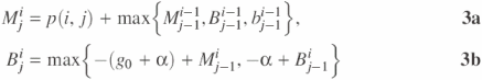
and

In this way, alignments with gaps in s use the B matrix and gaps in t use the b matrix. [Throughout this text, we have separate matrices for gaps/loops in s and t. If one imagines aligning s and t such that s is on top, as in Figure 1, then one can easily remember the differences between B and b with ‘uppercase B is for the upper sequence (s), and lowercase b is for the lower sequence (t)’.] Equation 3a fills the M matrix with the optimal alignment of s[1..i] and t[1..j], created either by adding yet another match or mismatch or by closing a gapped region grown in B or b with a match or mismatch. Equations 3b and 3c select the optimal way to align s[1..i] and t[1..j], either starting a new gapped region or extending an existing gap.

The alternative to adding extra matrices is explicitly searching over all n in Equation 2. This increases the computational complexity to O(|s|·|t|² + |s|²·|t|). Introducing the B and b matrices creates a finite state automaton, where each matrix corresponds to a state variable (24). In this case, the states are ending with a pair, with a gap in s or with a gap in t. Storing each state allows for efficient evaluation of competing structures, keeping the complexity O(|s|·|t|). This technique of using additional matrices avoids increasing the computational complexity and will play a key role in our bindigo algorithm.

The Turner rules we implement in bindigo are far more detailed than those above, with special conditions, exceptions and non-linear functions designed to reflect the physical reality of RNA binding. Although the basic structures can be broken down into base pairs, bulge loops, and internal loops the rules differ within each of these classes, requiring special attention to each case.

ALGORITHM

In this section we describe the bindigo algorithm, accessible at http://rna.williams.edu/. For maximum clarity, we give complementary presentations: the text description below the flowchart of Figure 2. The mathematical recursion relations are compiled in the online Supplementary Material. We begin here by detailing the structures and how they relate to the matrices used in bindigo, cross-referencing with Figure 2.

Figure 2.

This flowchart illustrates the bindigo algorithm, described in the text and in the recursion relations of online Supplementary Material, in terms of the matrices representing the different structures. An arrow into a matrix represents the free energy of the structure from the origin matrix feeding into the recursion relation of the destination. The numbers next to the arrow indicate the initial size of the loop considered by the matrix. Each alignment beginning with an initial stack (a) and concludes with a terminal stack (c), looping through base pairs (b) or bulge loops of various degrees of asymmetry (d–g) in between.

Base pairs

Base-pairing with stacking determines a nucleic acid's secondary structure. According to the nearest neighbor model, adjacent stacked base pairs have a well defined free energy (8). Nearest neighbor base pairs are analogous to Smith–Waterman matches, and the M matrix forms the hub of the algorithm. Matrix element M_jⁱ represents the best way to fold the prefixes s[1..i] and t[1..j] given that i and j are paired. Let the free energy of the nearest neighbors be given by the function NN(i, j), which, in the Turner rules, takes the form of a look-up table (8).

The very first or last base pair is called a terminal base pair and has a different free energy because the adjacent non-paired bases contribute to the net free energy (25). The special case of the first base pair accounts for the possibility that it may be optimal to incur the initiation penalty to ‘start afresh’, as illustrated in Figure 2a. [In the Turner rules there is fixed penalty to initially bring together two strands of RNA (8).] The final base pair is stored in the F matrix. F_jⁱ contains the free energy of the best way to align s[1..i] with t[1..j] given that no other bases are paired beyond i and j. As shown in Figure 2c, no other matrices depend on the F matrix, not even F itself. The minimum entry in the F matrix is the predicted optimal fold.

There is one more type of base-pairing, where the base pair is adjacent to an internal loop (9). Because these are always associated with an internal loop, we will discuss those when we address internal loops below.

Bulge loops

The Turner rules distinguish between two types of bulge loops: those with only one bulging base and those with multiple bulging bases. In the case of a single bulge, the free energy of the structure comes from the stacking of the base pairs on either end plus a fixed penalty (9). This is a special case within M matrix's recursion (Figure 2b).

Bulge loops longer than one base require an approach reminiscent of affine gaps, described in Equation 3, because their free energy depends entirely on their size (9). Figure 3 shows the function giving the penalty for bulge loops of a given size (26). Notice that the free energy penalty can be divided into two regimes, 2 ≤ n ≤ 6 and 6 < n. The free energy in each regime is quite linear, so that the bulge loop score is like an affine penalty in Smith–Waterman (27). We create two sets of matrices, illustrated in Figure 2d and e: B and b for bulge loops less than seven bases; and B2 and b2 for longer bulge loops. As shown in Figure 3, the scoring of B and b is optimal for 2 ≤ n ≤ 6, while B2 and b2 are optimal for n > 6.

Figure 3.

To a very good approximation, the free energy penalties of bulge loops can be described by the minimum of two linear relations. Notice that when a bulge loop is greater than 15 in size, the linearization scheme begins to differ slightly from Turner's rules (9). When less than 15, our linearization agrees exactly with experiment to within the 0.1 kcal/mol discretization of the Turner rules.

More specifically, these matrices represent the best way to align the prefixes s[1..i] and t[1..j] given that the alignment ends with a multiple-bulge loop but not a base pair. The closing pair is accounted for when the bulge rejoins M.

Internal loops

We distinguish among three classes of internal loops. First, there are the small loops whose energies have been tabulated for each possible sequence. These are the 1 × 1, 1 × 2, 2 × 1 and 2 × 2 loops. This notation indicates the numbers of unpaired bases (in s) × (in t) between the closing pairs. [The Turner group has investigated the free energies of individual 2 × 3 and 3 × 3 loops (28); however, these are not implemented in mfold 3.1 parameters (9).] We must check explicitly whether the optimal fold of s[1..i] and t[1..j] will end in one of these loops. Fortunately, there are only four of these, making this a computationally painless process. As Figure 2a shows, these are additional cases in the M matrix recursion.

The second class contains the n × 1 and 1 × n internal loops for n > 2. This requires two matrices: K for n × 1 loops and k for 1 × n loops. The free energy of these loops depends only on their size (see Figure 4). Unlike the bulge loops, an affine gap approach is infeasible. Instead, we look up the free energy difference between n and n + 1 in each case (see recursion relations in online Supplementary Material). Each K_jⁱ and k_jⁱ contains two components: free energy (K_jⁱ · dG) and the size of the loop (K_jⁱ · n). This performs well because the non-linearity is slight.

Figure 4.

The free energy penalty for n × m internal loops (where n and m are non-zero) depends on the total length of the loop, (n + m). These data are not well suited for the linearization strategy used for the bulge loops, as shown in Figure 3.

These matrices feed into M with the free energy is calculated as in this example with K_jⁱ. We can start a new 3 × 1 loop or extend the existing loop from n × 1 to (n + 1) × 1. These possibilities are illustrated in Figure 2f. If the optimal energy choice results from starting a new 3 × 1 loop, we set K_jⁱ · n = 3; otherwise, the loop grows by one, and K_jⁱ · n = K_jⁱ⁻¹ · n + 1.

The third and final type of asymmetric internal loop contains all internal loops larger than 2 × 2. The non-linear character of the general asymmetric internal loop free energy (9) again prevents us from using an affine gap technique. One approach to finding arbitrary internal loops is to explicitly cycle over every possible loop. To find the optimum in this way costs an undesirable O(|s|²·|t|²) operations. Placing a cap ℓ on internal loop size (11,29), would give O(ℓ²|s|·|t|) scaling. This, too, is undesirable because other researchers have determined that a reasonably sized ℓ is around 30 (29). Without imposing any cutoffs, we devised a useful heuristic that scales as O(|s|·|t|) with a prefactor equivalent to ℓ ≈ 4, much smaller than any reasonably sized ℓ².

We use two matrices, A and a, to ‘grow’ general n × m internal loops. As shown in Figure 2g, the A matrix is designated for growing the s side of the loop (n → n + 1), and the a matrix is for growing the t side (m → m + 1). Each entry in the A and a matrices has three numbers associated with it: the free energy of the loop (A_jⁱ · dG), the size of the loop in sequence s(A_jⁱ · n), and the size of the loop in sequence t(A_jⁱ · m). Any bonuses due to bases at the end of the loop, such as AU,GU helix closing penalties (8) are accounted for in M with the internal loop closing base pair free energy function, ilstack(i, j).

The policy for evaluating the components of each entry of A and a requires a more careful description due to its bipartite nature. The loops start at 3 × 2 or 2 × 3, because all smaller loops are handled by the mechanisms described earlier. The free energy aspect is treated similarly to 1 × n loops. Namely, as the loop grows, the energy due to the smaller loop is subtracted away and the energy of the new n × m loop is added (see recursion relations in online Supplementary Material).

Without this heuristic, we would have to explicitly calculate each possible internal loop up to ℓ × ℓ. Instead, we store asymmetric loop information in A_jⁱ and a_jⁱ. Only the locally optimal free energy is stored in these matrices, and multiple free energies compete for that value (see the recursion relations in the online Supplementary Material). Because of the nonlinearity of the internal loop rules (9), it is possible, though very rare, for a local minimum to displace the global minimum. However, because the optimal path takes many routes through the matrices, the likelihood of this worst case scenario is so remote that we are yet to observe it (see below).

RESULTS

Validation of heuristic

In order to establish the accuracy of our fast asymmetric loop heuristic, we compared the fast heuristic with a modified version using an explicit search, where we calculate

with ℓ = 30. We ran 30 000 random pairs of sequences of length 15, 25, 50 and 80, for a total of 120 000 trials. Each pair of sequences was run twice—once starting at s₀, t₀ and once with s and t interchanged so that the alignment is done from the other end of the sequences. If bindigo differed from the explicit version in both of these cases, that means the heuristic failed. Although sometimes the fast heuristic differed with the explicit search when binding in one direction, we never observed the case where it differed in both directions. (When run in a single direction only, the explicit and fast heuristic differed in 0.6% of the 15mers and 5% of the 80mers.) Hence, we are yet to observe a case where every way to fold a sequence disagrees with the lowest free energy fold given by the explicit version.

bindigo calculates inter-RNA binding using the same Turner free energy rules as mfold, so their predictions will not differ. Extensive comparison of bindigo with previously published mfold algorithms, in particular the PairFold server (20), provides us with our proof of correctness. Indeed, unless mfold predicts a hairpin loop, which we explicitly ignore for oligomeric binding, bindigo does not differ in its predictions.

Speed comparison: bindigo versus mfold

bindigo's decisive advantage over other RNA-binding algorithms is its speed. To compare the performance of bindigo and a modified mfold in analyzing oligomeric binding, we computed the binding affinity of the relevant portion of the splicesome's U1 sequence, t = AUACUUACCUGGC (12), to the Human Deoxyribonuclease-I precursor gene (NCBI accession number D83195). This RNA–RNA recognition event is, in general, required in precursor-mRNA splicing reactions (12,18). The time trials consisted of binding the relevant 13 bases of U1, t, to varying length subsequences of the gene (using one processor of an Apple PowerMac G5 with a 2.0 GHz PowerPC 970 and 2 GB of RAM). The results show the tremendous speed and scaling advantage of bindigo over mfold (Table 1).

Table 1. The time taken (ms) to bind the 13 nucleotide U1 to a subsequence of the human deoxyribonucleoase-I precursor gene of the given length.

Length	bindigo	mfold	Speedup
10	0.1 ms	22 ms	220
15	0.2 ms	25 ms	125
30	0.5 ms	30 ms	60
50	1.1 ms	53 ms	48
100	2.1 ms	153 ms	73
200	5.3 ms	580 ms	109
400	10.0 ms	2411 ms	241

mfold was run with the multiple molecule option, taking 25 copies of the same input. The timing was done using the user time of ‘time nafold’, then dividing by 25 in order to remove overhead due to loading datasets.

Analyzing splice sites with bindigo

The primary event in the pre-mRNA splicing process is when the U1 binds to the 5′ end of the intron (30). However, the U1 could bind to other parts of the pre-mRNA that are not splice sites. After all, a GU is the only conserved sequence at the 5′ splice site. bindigo's speed allows us to rapidly test hypotheses regarding the way the U1 binds to real sites versus decoy sites.

The probability of the U1 occupying a given location in the pre-mRNA is related to the free energy ΔG and chemical potential μ (12,31):

With bindigo, we can do more than simply look at splice sites and check their p_occ. For example, we can look at p_occ of positions surrounding the GU signal. Using a list of annotated splice sites (www.fruitfly.org/seq_tools/datasets/Human/GENIE_96), we composed substrings centered on every GU occurrence. One list contains the 1754 annotated real splice sites; the other, the first 90 000 decoy sites. We ran bindigo on all of the real and decoy sites, producing a p_occ for each position of a 102 nt window about each GU (50 nt before and 50 nt after).

The ΔG's we used came directly from the F matrix, according to

where t is the U1 and s is the windowed region surrounding the splice site. Thus ΔG_i = min_j(F_jⁱ) is the free energy of the best way to bind the U1 to the pre-mRNA given that s_i is the last paired base.

In order to compare the binding patterns of the U1 to real and decoy sites, we average p_occ at each j relative to the consensus GU for different values of μ/RT, as shown in Figure 5. There is a stark difference between real sites (Figure 5a) and decoy sites (Figure 5b). Most notably, decoy sites display a strong dependence on decreasing the U1 concentration, corresponding to decreasing μ/RT; the peak in 〈p_occ〉 for decoys disappears while the peak in 〈p_occ〉 for reals remains. Thus, a low-cellular U1 concentration enhances the U1's relative affinity to real splice sites over decoy sites. Note also that the peak in the decoy sites is also displaced upstream of the peak associated with real sites, indicating a slight difference in the average secondary structure. This agrees with the observation that the secondary structure about the GU plays a key role in the specificity of the U1 (12).

Figure 5.

The predicted average occupation probabilities (Equation 5) of the U1 snRNA at (a) 1754 real splice sites or (b) 90 000 decoy sites is plotted for different values of the chemical potential μ. As the U1 concentration decreases, corresponding to a smaller μ/RT, binding affinity drops dramatically. Position i is the last paired base of the U1 on a scale where positions 1 and 2 are the conserved GU. The U1 clearly binds more strongly to and to more bases of reals than decoys.

As mentioned above, p_occ(i) corresponds to the last base paired in the pre-mRNA. By interchanging s and t, p_occ(i) gives information on the first base paired. Our plot of both the 3′ and 5′ versions of p_occ is given in Figure 6. The U1 almost always straddles the GU signal in real splice sites with well-defined beginning and ending locations. The 5′ end of the U1 tends to site 3 or 4 bases upstream of the GU signal, while the 3′ end is 6 to 8 bases downstream. This has also been observed in statistical models for splice site detection (32).

Figure 6.

The average occupation probability p_occ indicates the last base paired i. The 3′ curve reveals that U1 binding terminates typically at positions 6 or 8, where positions 1 and 2 are the conserved GU. Computing binding right to left (5′ curve), by interchanging s and t, shows that U1 typically involves 4 bases of the intron.

DISCUSSION

With the framework we have presented here, we can take advantage of bindigo's speed to solve a myriad of problems. We have just demonstrated with our analysis of the U1 binding to GU signals that bindigo is ideally suited for dealing with vast libraries of oligomeric sequences. By using bindigo to study thousands of potential donor splice sites, we observed key differences between the U1 binding to reals and decoys. By maintaining a low concentration of U1, the cell can optimize the U1's specificity for real splice sites. In addition the U1 shows much stronger binding downstream of a real GU signal compared to upstream binding, while no such difference exists for false GU's. These differences could be used in a selection algorithm similar to Garland and Aalbert's (12) ‘Finding with Binding’ splice site detection.

Although here we have provided extensive details of RNA–RNA binding, we have also created a version of bindigo that handles DNA–DNA binding. The only changes required were to use the available DNA–DNA datasets (33–38). There is no 1 × n loop rule for DNA, so that separate structure was omitted. bindigo will be a useful tool for studying many RNA and DNA problems in computational biology including RNA interference, DNA microarray thermodynamics, splice site detection and transposons.

It appears feasible to use bindigo in conjunction with mfold to produce a powerful, more sophisticated, binding algorithm that addresses the following fundamental limitation: an oligo binding to an internal loop or hairpin loop is analogous to a pseudoknot (Figure 7). Given a very large RNA, s, and an oligo, t, we may avoid this limitation by first folding s alone with mfold in the usual way. mfold produces a matrix W_ii′, which is the free energy of the optimal fold of all bases between s_i and s_i′, inclusive. Importantly, when i′ > i, W_i′i is the free energy of binding all of the bases except for those between s_i and s_i′, exclusive.

Figure 7.

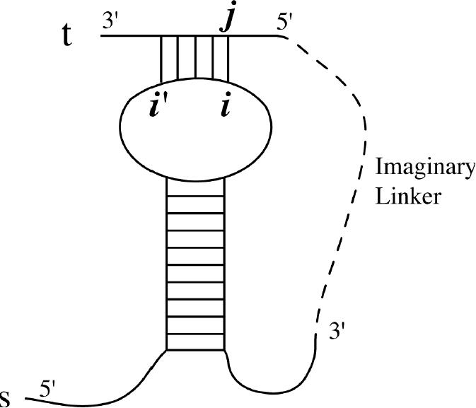
In an mfold-type binding algorithm, sequences s and t are joined by an imaginary linker, as shown, and folded as a single chain. If the optimal free energy binding were for s to form a hairpin and t to bind to the loop; then the minimum free energy structure would be a pseudoknot, a structure which cannot be found with most existing folding algorithms.

Our proposed procedure is to use bindigo to obtain all valid combinations of s and t, in F_jⁱ. This binding free energy is added to the free energy of the rest of s plus a correction term for the geometry of the fold,

After the addition of a one-time cost of O(|s|³) to mfold s, this new approach scales as O(|s|³ + |s|·|t|). A few technical challenges to this approach are remedying the mfold assumption that W_i′i is a multiloop, storing the first paired base i′ and other information about the loop length in the recursion matrices. This combined method avoids the inherent limitations of ordinary binding algorithms, with minimal computational penalty.

SUPPLEMENTARY MATERIAL

Supplementary Material is available at NAR online.

REFERENCES

- 1.Smith T.F. and Waterman,M.S. (1981) The identification of common molecular subsequences. J. Mol. Biol., 147, 195–197. [DOI] [PubMed] [Google Scholar]
- 2.Sniedovich M. (1992) Dynamic Programming. Marcel Dekker, NY. [Google Scholar]
- 3.Zuker M. and Stiegler,P. (1981) Optimal computer folding of large RNA sequences using thermodynamics and auxiliary information. Nucleic Acids Res., 9, 133–148. [DOI] [PMC free article] [PubMed] [Google Scholar]
- 4.Hofacker I.L., Fontana,W., Standler,P.F., Bonhoeffer,L.S., Tacker,M. and Schuster,P. (1994) Fast folding and comparison of RNA secondary structures. Monatsh. Chem., 125, 167–188. [Google Scholar]
- 5.Zuker M. (2000) Calculating nucleic acid secondary structure. Curr. Opin. Struct. Biol., 10, 303–310. [DOI] [PubMed] [Google Scholar]
- 6.McCaskill J.S. (1990) The equilibrium partition function and base pair binding probabilities for RNA secondary structure. Biopolymers, 29, 1105–1119. [DOI] [PubMed] [Google Scholar]
- 7.Rivas E. and Eddy,S.R. (1999) A dynamic programming algorithm for RNA structure prediction including pseudoknots. J. Mol. Biol., 285, 2053–2068. [DOI] [PubMed] [Google Scholar]
- 8.Xia T., SantaLucia,J.,Jr, Burkard,M.E., Kierzek,R., Schroeder,S.J., Jiao,X., Cox,C. and Turner,D.H. (1998) Thermodynamic parameters for an expanded nearest-neighbor model for formation of RNA duplexes with Watson–Crick base pairs. Biochemistry, 37, 14719–14735. [DOI] [PubMed] [Google Scholar]
- 9.Mathews D.H., Sabina,J., Zuker,M. and Turner,D.H. (1999) Expanded sequence dependence of thermodynamic parameters improves prediction of RNA secondary structure. J. Mol. Biol., 288, 911–940. [DOI] [PubMed] [Google Scholar]
- 10.Lyngsø R.N. and Pedersen,C.N.S. (2000) Pseudoknots in RNA secondary structures. In Proceedings of the Fourth International Conference on Computational Molecular Biology (RECOMB'00), 8–11 April, Tokyo, Japan, pp. 201–209. [Google Scholar]
- 11.Lyngsø R.B., Zuker,M. and Pedersen,C.N.S. (1999) Fast evaluation of internal loops in RNA secondary structure prediction. Bioinformatics, 15, 440–445. [DOI] [PubMed] [Google Scholar]
- 12.Garland J.A. and Aalberts,D.P. (2004) Thermodynamic modeling of donor splice site recognition in pre-mRNA. Phys. Rev. E, 69, 041903. [DOI] [PubMed] [Google Scholar]
- 13.Lewis B.P., Shih,I.-h., Jones-Rhoades,M.W., Bartel,D.P. and Burge,C.B. (2003) Prediction of mammalian microRNA targets. Cell, 115, 787–798. [DOI] [PubMed] [Google Scholar]
- 14.Couzin J. (2002) Small RNAs make big splash. Science, 298, 2296–2297. [DOI] [PubMed] [Google Scholar]
- 15.Ketting R.F., Fischer,S.E.J., Bernstein,E., Sijen,T., Hannon,G.J. and Plasterk,R.H.A. (2001) Dicer functions in RNA interference and in synthesis of small RNA involved in developmental timing in C. elegans. Genes Dev., 15, 2654–2659. [DOI] [PMC free article] [PubMed] [Google Scholar]
- 16.Brown T.A. (2002) Genomes, 2nd edn. Wiley, NY. [Google Scholar]
- 17.Ichiyanagi K., Beauregard,A., Lawrence,S., Smith,D., Cousineau,B. and Belfort,M. (2002) Retrotransposition of the Ll. LtrB group II intron proceeds predominantly via reverse splicing into DNA targets. Mol. Microbiol., 46, 1259–1272. [DOI] [PubMed] [Google Scholar]
- 18.Lodish H., Berk,A., Matsudaira,P., Kaiser,C.A., Krieger,M., Scott,M.P., Zipursky,S.L. and Darnell,J. (2004) Molecular Cell Biology, 5th edn. W.H. Freeman and Company, NY. [Google Scholar]
- 19.Lowe T.M. and Eddy,S.R. (1999) A computational screen for methylation guide snoRNAs in yeast. Science, 283, 1168–1173. [DOI] [PubMed] [Google Scholar]
- 20.Andronescu M., Aguirre-Hernández,R., Condon,A. and Hoos,H.H. (2003) RNAsoft: a suite of RNA secondary structure prediction and design software tools. Nucleic Acids Res., 31, 3416–3422. [DOI] [PMC free article] [PubMed] [Google Scholar]
- 21.Mathews D.H., Burkard,M.E., Freier,S.M., Wyatt,J.R. and Turner,D.H. (1999) Predicting oligonucleotide affinity to nucleic acid targets. RNA, 5, 1458–1469. [DOI] [PMC free article] [PubMed] [Google Scholar]
- 22.Zuker M. (2003) Mfold web server for nucleic acid folding and hybridization prediction. Nucleic Acids Res., 31, 3406–3415. [DOI] [PMC free article] [PubMed] [Google Scholar]
- 23.Gotoh O. (1982) An improved algorithm for matching biological sequences. J. Mol. Biol., 162, 705–708. [DOI] [PubMed] [Google Scholar]
- 24.Durbin R., Eddy,S., Krogh,A. and Mitchison,G. (1998) Biological Sequence Analysis, Chapter 2. Cambridge University Press, Cambridge. [Google Scholar]
- 25.Serra M.J. and Turner,D.H. (1995) Predicting thermodynamic properties of RNA. Methods Enzymol., 259, 242–261. [DOI] [PubMed] [Google Scholar]
- 26.Jacobson H. and Stockmayer,W.H. (1950) Intramolecular reaction in polycondensations. I. The theory of linear systems. J. Chem. Phys., 18, 1600–1606. [Google Scholar]
- 27.Meudanis J. and Setubal,J.C. (1997) Introduction to Computational Molecular Biology, Chapter 3. PWS Publishing Co., Boston, MA. [Google Scholar]
- 28.Schroeder S.J. and Turner,D.H. (2000) Factors affecting the thermodynamic stability of small asymmetric internal loops in RNA. Biochemistry, 39, 9257–9274. [DOI] [PubMed] [Google Scholar]
- 29.Lyngsø R.B., Zuker,M. and Pedersen,C.N.S. (1999) Internal loops in RNA secondary structure prediction. In Proceedings of the Third International Conference in Computational Molecular Biology (RECOMB'99), pp. 260–267. [Google Scholar]
- 30.Nagai K., Muto,Y., Pomeranz Krummel,D.A., Kambach,C., Ignjatovic,T., Walke,S. and Kuglstatter,A. (2001) Structure and assembly of the spliceosomal snRNPs. Biochem. Soc. Trans., 29, 15–26. [DOI] [PubMed] [Google Scholar]
- 31.Schroeder D.V. (2000) An Introduction to Thermal Physics. Addison Wesley Longman, San Francisco, CA. [Google Scholar]
- 32.Burge C.B., Tuschl,T. and Sharp,P.A. (1999) Splicing of precursors to mRNAs by the splicesomes. In Gesteland,R.F., Cech,T.R. and Atkins,J.F. (eds) The RNA World, 2nd Edn. Cold Spring Harbor Laboratory Press, Cold Spring Harbor, NY. [Google Scholar]
- 33.SantaLucia J., Allawi,H.T. and Senevirante,A. (1996) Improved nearest-neighbor parameters for predicting DNA duplex stability. Biochemistry, 35, 3555–3562. [DOI] [PubMed] [Google Scholar]
- 34.Allawi H.T. and SantaLucia,J.,Jr (1997) Thermodynamics and NMR of internal GT mismatches in DNA. Biochemistry, 34, 10581–10594. [DOI] [PubMed] [Google Scholar]
- 35.Allawi H.T. and SantaLucia,J.,Jr (1997) Nearest neighbor thermodynamic parameters for internal G·A mismatches in DNA. Biochemistry, 37, 2170–2179. [DOI] [PubMed] [Google Scholar]
- 36.Allawi H.T. and SantaLucia,J.,Jr (1998) Thermodynamics of internal C·T mismatches in DNA. Nucleic Acids Res., 11, 2694–2701. [DOI] [PMC free article] [PubMed] [Google Scholar]
- 37.Allawi H.T. and SantaLucia,J.,Jr (1998) Nearest-neighbor thermodynamics of internal A·C mismatches in DNA: sequence dependence and pH effects. Biochemistry, 26, 9435–9444. [DOI] [PubMed] [Google Scholar]
- 38.Peyret N., Seneviratne,P.A., Allawi,H.T. and SantaLucia,J. (1999) Nearest-neighbor thermodynamics and NMR of DNA sequences with internal A·A, C·C, G·G, and T·T mismatches. Biochemistry, 38, 3468–3477. [DOI] [PubMed] [Google Scholar]
Associated Data
This section collects any data citations, data availability statements, or supplementary materials included in this article.