Determinants of Rotavirus Transmission

Supplemental Digital Content is available in the text.

Abstract

Rotavirus is a common viral infection among young children. As in many countries, the infection dynamics of rotavirus in the Netherlands are characterized by an annual winter peak, which was notably low in 2014. Previous study suggested an association between weather factors and both rotavirus transmission and incidence. From epidemic theory, we know that the proportion of susceptible individuals can affect disease transmission. We investigated how these factors are associated with rotavirus transmission in the Netherlands, and their impact on rotavirus transmission in 2014. We used available data on birth rates and rotavirus laboratory reports to estimate rotavirus transmission and the proportion of individuals susceptible to primary infection. Weather data were directly available from a central meteorological station. We developed an approach for detecting determinants of seasonal rotavirus transmission by assessing nonlinear, delayed associations between each factor and rotavirus transmission. We explored relationships by applying a distributed lag nonlinear regression model with seasonal terms. We corrected for residual serial correlation using autoregressive moving average errors. We inferred the relationship between different factors and the effective reproduction number from the most parsimonious model with low residual autocorrelation. Higher proportions of susceptible individuals and lower temperatures were associated with increases in rotavirus transmission. For 2014, our findings suggest that relatively mild temperatures combined with the low proportion of susceptible individuals contributed to lower rotavirus transmission in the Netherlands. However, our model, which overestimated the magnitude of the peak, suggested that other factors were likely instrumental in reducing the incidence that year.

Rotavirus generally infects unvaccinated children initially between 6 and 24 months of age, and nearly always before 5 years of age.¹ Reinfections are generally less severe than the first episodes, with primary rotavirus infection accounting for an estimated 86% of the moderate-to-severe diarrhea associated with rotavirus.^1,2 As in many countries, the infection dynamics of rotavirus in the Netherlands are characterized by predictable annual winter peaks in reported incidence that vary in height and breadth. In 2014, the pattern of rotavirus incidence in England and in the Netherlands was notably different from that of previous years.^3,4 In England, the substantially lower reported incidence was attributed to the introduction of an infant rotavirus vaccine in July 2013.³ The reason for the nearly identically low reported incidence in the Netherlands is less clear because the uptake of rotavirus vaccine among Dutch infants has been negligible to date.

A preliminary look at data (Figure 1) suggested two hypotheses for this observation. First, previous study has suggested that lower temperatures are associated with increased rotavirus transmission and incidence, with the effect of colder temperatures lasting for up to 1 or 4 weeks, respectively.^5–10 If temperature indeed (indirectly) affects rotavirus incidence,⁶ then the unusually mild winter temperatures in 2014 contributed to the relatively low rotavirus incidence that year. However, it is unclear whether prior analyses corrected for residual serial correlation. Generally, for time series data, the residuals of classical regression are correlated over time. Failing to correct for these correlations violates the independent errors assumption, and generates, at least, incorrect confidence intervals that are too narrow and statistical tests that overstate the significance of the regression coefficients, and, at most, spurious associations.^11–13

FIGURE 1.

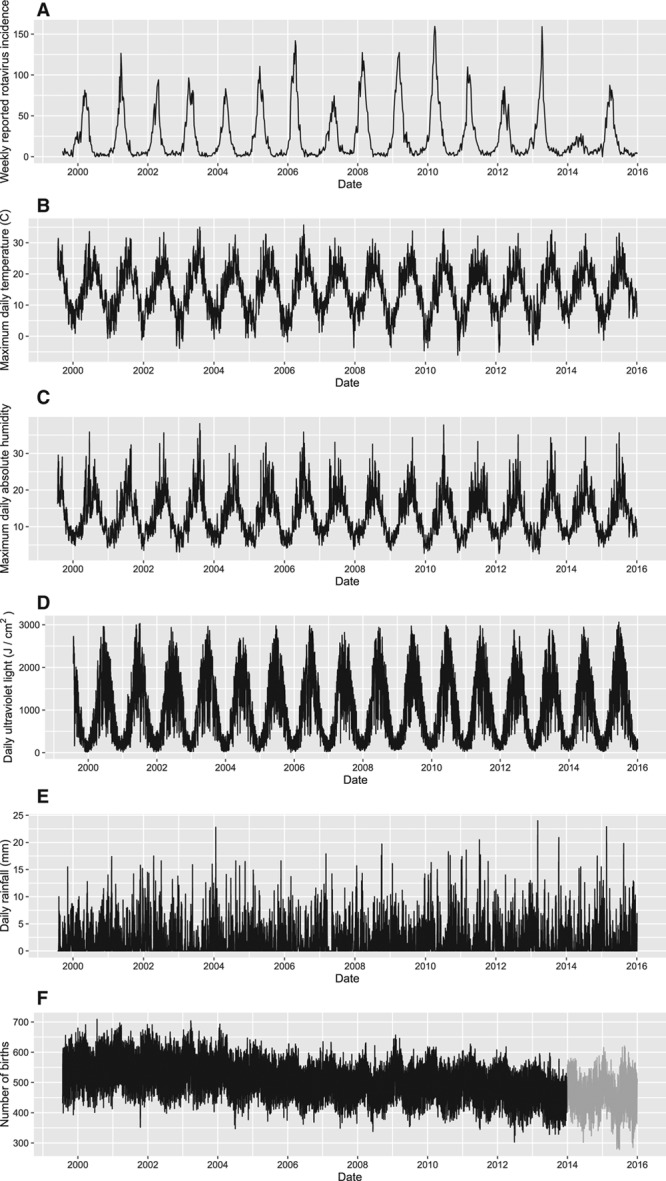
Available time series data over the period 1999–2015 in the Netherlands. A, Reported rotavirus incidence by week for the Netherlands, weighted according to the number of the laboratories reporting in any given week. B, Maximum daily temperature recorded at the meteorological station in De Bilt, the Netherlands. C, Maximum daily absolute humidity recorded at the meteorological station in De Bilt, the Netherlands. D, Daily ultraviolet light recorded at the meteorological station in De Bilt, the Netherlands. E, Daily rainfall recorded at the meteorological station in De Bilt, the Netherlands. F, Actual number of births per day in the Netherlands 2000–2013 (black), including the simulated number of births per day for 2014–2015 (grey).

Second, a lower proportion of susceptible individuals is associated with a lower incidence of infection at some future time depending on the duration of the incubation period.¹⁴ The relatively high incidence in 2013 may have left fewer individuals susceptible to primary infection, leading to a lower reported incidence in 2014.

A useful metric to estimate the transmissibility of infectious diseases is the effective reproduction number, R(t) defined as the average number of secondary cases produced by any one infectious case at time t. An epidemic is under control and incidence decreases when R(t) < 1.

Here, we set out to disentangle possible effects of weather factors and the proportion of susceptible individuals (factors) on the effective reproduction number of rotavirus (outcome) in the Netherlands. We assessed whether past values of a factor are more strongly associated with the current value of an outcome than the past values of the outcome itself by assessing Granger causality.¹⁵ Throughout our analyses, we applied a strict test for detecting associations by explicitly correcting the regression residuals for serial correlation using autoregressive moving average methods.

METHODS

We first describe data available and the methods used to estimate required data from available data. We then present the statistical methods used to test for associations.

Available Data

Rotavirus Incidence

Data on weekly reported rotavirus detections from July 27, 1999 to December 31, 2015 were obtained from the Dutch Working Group for Clinical Virology. This database contains data on the number of individuals with stool testing positive for rotavirus from 17 to 21 virology laboratories in the Netherlands. Reported test-positive incidence data were weighted by the number of laboratories reporting per week, and were then used as a proxy for incidence of the event of interest: a primary rotavirus infection.

Weather Data

Data on the maximum, minimum, and average daily temperature and absolute humidity, ultraviolet light, and rainfall from January 1, 1950 to December 31, 2015 were available from the Royal Netherlands Meteorological Institute. We used data from the meteorological station in De Bilt, located in the middle of the Netherlands and considered representative for the country.

Number of Births

Data on the daily number of births in the Netherlands from January 1, 1995 to December 31, 2013 were obtained from Statistics Netherlands. For 2014–2015, only monthly birth rate data were available. Daily birth rate data for these years were estimated using the available monthly data and the daily trends from previous years. See eAppendix B (http://links.lww.com/EDE/B186) for additional details.

The study period that we considered in this analysis was from 1 January 2000 to 31 December 2015, providing us with a large dataset for our analyses. No ethical approval was required. Original time series data on the weighted reported rotavirus incidence, maximum daily temperature, maximum absolute humidity, ultraviolet light, rainfall, and birth rate are shown in Figure 1. Note the low reported rotavirus incidence in 2014 (Figure 1A), which coincided with a relatively mild winter (Figure 1B). In addition to the clear yearly trend observed in each time series plot, the daily number of births gradually decreased over time. We expected the temperature and the proportion of susceptible individuals to directly affect rotavirus transmission. We additionally evaluated the effect of variables for which we did not expect to observe an association, including ultraviolet light, rainfall, and absolute humidity. We did not assess the effect of school vacations because most primary infections occur before children are old enough to attend school.

Estimating the Proportion of Susceptible Individuals

The primary infection with rotavirus is the most likely to be symptomatic and severe. Therefore, in calculating the proportion of susceptible individuals from the weekly number of reported rotavirus cases, we made two assumptions: (1) the majority of cases represented in our reported rotavirus incidence data were of primary infections and (2) individuals were removed from the population at risk for severe infection after their primary infection. Sensitivity of our results to this second assumption was assessed in eAppendix E (http://links.lww.com/EDE/B186). Because infants younger than 6 months are generally protected from rotavirus infection due possibly to maternal immunity,^16–18 children older than 6 months who had never been infected constituted the susceptible population in our analysis.

The infection dynamics described above are akin to a standard epidemic susceptible-infected-recovered model, common in mathematical modeling.¹⁹ The absolute number of susceptible individuals for any given week S(t) was calculated as the number of susceptible individuals at the start of follow-up (S₀), plus the cumulative number of individuals older than 6 months of age (δ) from the start of our time series to week t subtracted by the cumulative number of rotavirus cases (I) from the start of our time series to week t We estimated S₀ as the average expected duration in the susceptible class (9 months, discussed below) times the average daily number of new susceptible individuals in 1999.

Reported rotavirus incidence data (I_r) underestimate primary rotavirus infection in the Netherlands: not all Dutch laboratories report to the database and laboratory tests are conducted on a small fraction of all individuals with rotavirus. To estimate the proportion of case ascertainment at each week α(t), we used local linear regression of births versus rotavirus cases. Because all individuals become infected with rotavirus and primary infections occur shortly after individuals become susceptible, the ratio of cases to births estimates well the case ascertainment.²⁰ For our main analysis, we set to 9 months the average time that individuals are expected to be susceptible to primary infection. In eAppendix E (http://links.lww.com/EDE/B186), we tested the sensitivity of our results to alternative average durations in the susceptible class.

We adjusted the number of reported cases for under-ascertainment to arrive at a balance equation for the number of susceptible individuals:

Because all children are infected with rotavirus at least once before 5 years of age, we set the time-dependent denominator of the total number of individuals in the population N(t) to be the total number of births in the Netherlands in the previous 5 years. Therefore, the proportion of susceptible individuals at week t was S(t)/N(t). In eAppendix B (http://links.lww.com/EDE/B186), we show how α(t) changes over time.

Estimating the Effective Reproduction Number of Rotavirus

The effective reproduction number, R(t), measures the number of secondary cases infected per primary case at time t and can be calculated as²¹

where Î(u) is the rotavirus infection incidence at time u and g(u) is the probability density of the generation interval distribution at time u, which we calculated in eAppendix B (http://links.lww.com/EDE/B186). The mean of the generation interval was 2.1 days (SD = 0.9), which agrees with the estimated rotavirus incubation period of 2 days.¹ In eAppendix E (http://links.lww.com/EDE/B186), we tested the sensitivity of our results to a longer generation interval. Because the mean of the generation interval distribution was less than 1 week, we converted weekly incidence data into daily data using a smoothing spline to estimate R(t), and then averaged R(t) by week. To reduce the impact of noise on our results during periods of low incidence, we smoothed the effective reproduction number over time using Bayesian integrated nested Laplace approximations models.^22,23 (Reasoning and details are available in eAppendix B; http://links.lww.com/EDE/B186.)

Statistical Analysis

Throughout our analyses, we considered as outcome the log effective reproduction number of rotavirus, log(R(t)), and as factors the log proportion of susceptible individuals, ultraviolet light, rainfall, the maximum, minimum, and mean temperature and absolute humidity. Because the original reported rotavirus incidence data were aggregated by week, our analyses relied on weekly data (eFigure 15; http://links.lww.com/EDE/B186). Here, we outline preliminary analyses used to construct methods for our main analysis, described in the rest of this subsection.

Preliminary Analyses: Granger Causality

We assessed Granger causality for each factor F using

(1)

for the number of lags l that optimized model fit according to the Akaike Information Criterion (AIC). A factor is considered to Granger-cause log(R(t)) if at least one β_i,i = 1,2,…,l is statistically different from zero. Our analyses suggested a Granger causal association between log(R(t)) and all factors considered except rainfall. Notice that because the Granger model does not account for seasonality, it may detect spurious associations.

Preliminary Analyses: Simulation Study

Using simulations, we assessed the effect of correcting for residual serial correlation (described in eAppendix A; http://links.lww.com/EDE/B186). Our analyses demonstrated that (1) failing to account for serial correlation increased the probability of identifying an association when there was none (i.e., increased false positive rate), (2) accounting for serial correlation did not reduce the probability of detecting an association when there was one (i.e., did not increase the false negative rate), and (3) accounting for serial correlation improved the probability of correctly identify the nature of associations (e.g., whether the effect of a factor was immediate or delayed).

Regression Model

For our main analysis, we used a regression model to first assess the linear immediate and 1-week delayed association between each factor and log(R(t)). We then tested for nonlinear and delayed associations using flexible natural splines.²⁴ We adjusted for yearly (seasonal) correlation using m_s sine terms and m_c cosine terms with a period of 52.2 weeks. Thus, our regression model was as follows:

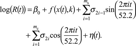(2)

In this equation, β₀ is the underlying constant level of rotavirus transmission in the Dutch population over time, each σ_i represents the seasonal effect contributed by the corresponding sine or cosine term, and η(t) denotes the error terms of the regression model. The number of sine and cosine terms included in the model was selected using the AIC. f(x(t),k) denotes either a linear (immediate or delayed) effect or a time-dependent natural cubic spline x(t) of the factor with k degrees of freedom (hereafter: “functional form”). For each factor included in the regression model, the selected functional form yielded optimal model fit (lowest AIC).

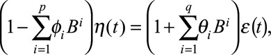
Accounting for Serial Correlation

As written, the ordinary regression model (Equation 2) assumes independent residuals, which is generally an invalid assumption for time series analyses. We augmented Equation 2 to automatically correct the regression estimates for autocorrelation, such that the residuals were modeled using autoregressive moving average terms:

(3)

where the p autoregressive terms account for correlation between p consecutive weeks, the q moving average terms account for correlation between the regression errors between q consecutive weeks, η(t) refers to the error terms from the regression equation (Equation 2), and ε(t) denotes normally and independently distributed error terms. Note that 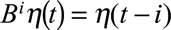and 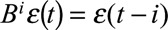. For a given (set of) factor(s) and prespecified values for m_s, m_c, p, q, and k, all coefficients of these regression models, Equations 2 and 3, were iteratively estimated using the Arima function in R 3.1.0 such that model fit was optimized (lowest AIC).

Model Selection

Along with analyses using one factor in the regression model (“univariate” analyses), we combined the different factors into one multivariate model to assess the combined effect. The best model was the one that had the lowest AIC and relatively low (partial) autocorrelation. We used Q–Q plots to ensure that our final model had normally distributed errors.

Finally, we used a 28-week moving average of the results of the regression model (Equation 2) to suggest time periods where the model was insufficient to explain, on average, the observed trends in the effective reproduction number. Further details are provided in eAppendix B (http://links.lww.com/EDE/B186).

All statistical analyses were conducted in R 3.1.0, using the tseries, splines, INLA, forecast, and dlnm packages.^25–29 Example code is provided in eAppendix C (http://links.lww.com/EDE/B186).

RESULTS

Estimated Proportion of Susceptible Individuals and Effective Reproduction Number

We estimated that approximately 150,000 individuals in the Netherlands were susceptible to rotavirus at the start of our time series. An estimate of the proportion of susceptible individuals over time (Figure 2) shows that the proportion of susceptible individuals generally peaks just before the start of a new rotavirus season when rotavirus incidence is still low (December–January) and reaches a trough at the end of the rotavirus season (April–May). An anomaly was observed in 2014, where the proportion of susceptible individuals continued to increase well into the usual epidemic months, and peaked when rotavirus incidence (mildly) peaked that year. The gradual decline was partially caused by a reduced influx of new susceptible individuals (6-month-olds) in the first half of 2014. In Figure 3, we plotted the time-dependent log effective reproduction number of rotavirus calculated using Bayesian integrated nested Laplace approximations models, which was the outcome in our analyses. Clear seasonal patterns were observed in Figures 2 and 3.

FIGURE 2.

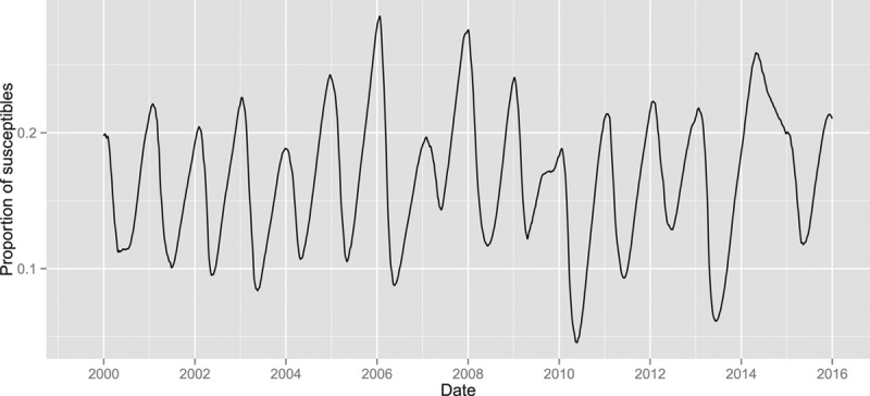
Proportion of susceptible individuals over time, S(t)/N(t), calculated using an estimate of the number initially susceptible and the estimated proportion of case ascertainment.

FIGURE 3.

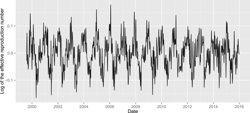
Log of the effective reproduction number, R(t), estimated using Bayesian integrated nested Laplace approximations models.

Regression Modeling with Autoregressive Moving Average Errors

Using “univariate” regression models that accounted for seasonality and serial correlation, we found that natural cubic splines with three degrees of freedom provided the best fit for both the log proportion of susceptible individuals and minimum, maximum, and mean temperature. Optimal model fit was obtained when a delay of up to 2 weeks for temperature and when a delay of up to 3 weeks for the log proportion of susceptible individuals were included in the model (eFigure 16; http://links.lww.com/EDE/B186). Delayed effects were also modeled using a natural cubic spline with three degrees of freedom. The effect of the proportions of susceptible individuals fluctuated from week to week. Therefore, we calculated the total current and delayed effect of each proportion of susceptible individuals. We observed that weeks with higher proportions of susceptible individuals were associated with a higher effective reproduction number (eFigure 16a; http://links.lww.com/EDE/B186). Furthermore, the shapes of splines suggest that lower temperatures in the current and previous week were associated with a higher log(R(t)) (eFigure 16b–d; http://links.lww.com/EDE/B186). There was no evidence of an immediate or delayed association between ultraviolet light, rainfall, and absolute humidity and log(R(t)) (eFigure 16e–i; http://links.lww.com/EDE/B186).

Next, we considered multivariate models that accounted for seasonality and serial correlation. The model with the best fit, and therefore selected as our final model, included the log proportion of susceptible individuals and mean temperature, modeling their effects using a natural cubic spline with three degrees of freedom. Optimal model fit was obtained when temperature with a delay of up to 2 weeks and the log proportion of susceptible individuals with a delay of up to 3 weeks were included in the model. In eAppendix D (http://links.lww.com/EDE/B186), we compare results of multivariate models with different numbers of delayed terms. Ultraviolet light, rainfall, and absolute humidity were not associated with the effective reproduction number of rotavirus. The remainder of this section presents findings based on this final model.

The shapes of the splines representing the total effects of mean temperature and the proportion of susceptible individuals (Figure 4), which were nearly identical to the univariate models, suggest that higher proportions of susceptible individuals and lower temperatures were associated with a higher log(R(t)) The estimated total effect of a high current proportion of susceptible individuals (e.g. 0.27) was an increase in log(R(t)) of 0.03 relative to the average proportion of susceptible individuals (0.11) (Figure 4A). The estimated effect of low temperatures (e.g., −7°C) on log(R(t)) was an increase in log(R(t)) of 0.075 relative to the average temperature (16°C) (Figure 4B). Similar results were observed for models with different numbers of delayed terms (eFigures 19–21; http://links.lww.com/EDE/B186). Additional results of our final model, including the estimated coefficients, are available in eAppendix D (http://links.lww.com/EDE/B186).

FIGURE 4.

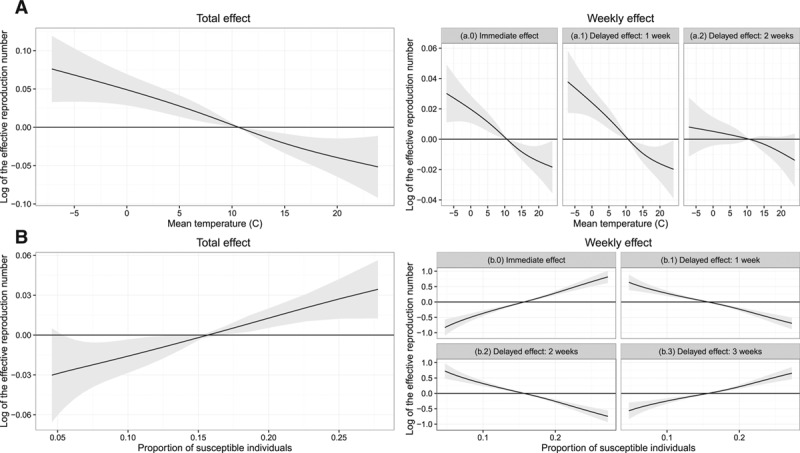
The total, immediate, and delayed effect on the effective reproduction number, R(t), of the (A) proportion of susceptible individuals S(t)/N(t) and (B) mean temperature, as estimated in our best-fitting model that corrected for serial correlation and included terms for seasonality. The black line represents the estimated effect, and the grey region indicates the 95% confidence intervals.

We combined the estimated effects of the proportion of susceptible individuals and of mean temperature on the effective reproduction number to arrive at an estimated critical threshold, where R(t) = 1. Assuming a negligible effect of seasonality and serial correlation on R(t) this critical threshold suggests the proportion of susceptible individuals and the mean temperature for which an epidemic could change from increasing to decreasing incidence. The shaded region in Figure 5 shows the proportion of susceptible individuals and the mean temperature for which our model suggests this critical shift could occur. For example, a proportion of susceptible individuals equal to 0.10 may be sufficient to reduce the effective reproduction number to below one for all mean temperatures above 6.7°C (95% confidence interval [CI] = 2.5°C, 9.3°C; Figure 5).

FIGURE 5.

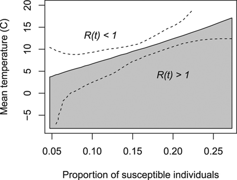
The proportion of susceptible individuals and the mean temperature for which our model suggests an increasing incidence (effective reproduction number above one; in grey) and a decreasing incidence (below one; in white), assuming the effect of the seasonality on the effective reproduction number was equal to one and the effect of serial correlation equals one. Dashed lines depict the 95% confidence interval.

In the following two paragraphs, we break down the contribution of different variables in explaining log(R(t)) variability over time in the final model. Separate graphs of the explanatory value of the proportion of susceptible individuals and mean temperature in estimating log(R(t)) time trends show a clear seasonal trend (Figure 6). Together these two factors alone explain up to the total magnitude of log(R(t)) at its peak (Figure 7A). The year 2014 was an anomaly: the unusually low rotavirus incidence during the 2014 season left the highest proportion of individuals susceptible to infection at the end of the rotavirus season in the 15 years for which data were available (Figures 2 and 6A). The high proportion of susceptible individuals suggests that epidemic-level rotavirus transmission (R(t) > 1) could have continued into the summer, and perhaps through most of the year (Figure 6A). When considering this factor along with temperature, it appears as though the warmer summer weather reduced the effective reproduction number to below one.

FIGURE 6.

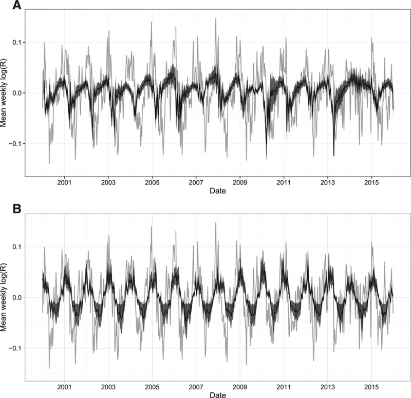
A breakdown of the effect of the variables included in our final model compared with the effective reproduction number (grey). A, The estimated effect of the log proportion of susceptible individuals. B, The estimated effect of the mean temperature.

FIGURE 7.

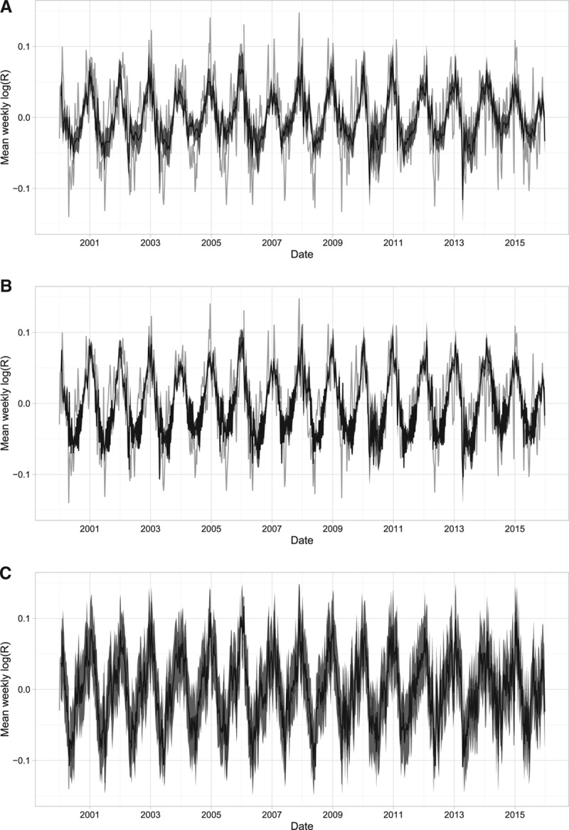
A breakdown of the effect of the variables included in our final model compared with the effective reproduction number (grey). A, The estimated effect of the log average weekly proportion of susceptible individuals and the average weekly mean temperature. B, The estimated effect of the proportion of susceptible individuals, mean temperature, and seasonality. C, The fit of the complete, best-fitting model, including serial correlation correction.

The proportion of susceptible individuals, mean temperature, and seasonal effects alone did not completely capture the week-to-week variability in the effective reproduction number (Figure 7B). When we additionally considered the effects of serial correlation, we observed a closer approximation of the week-to-week variability (Figure 7C). When the estimated combined effect of the proportion of susceptible individuals, mean temperature, and seasonal factors were averaged over 28 weeks, we observed that they generally followed the peaks of the 28-week average effective reproduction number (Figure 8). Our final model overestimated the peak in 2014, which may suggest that the reduction in the effective reproduction number that year may have been caused by factors not included in our analysis.

FIGURE 8.

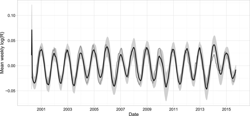
The 28-week moving average of the estimated effective reproduction number of rotavirus (grey) and the 28-week moving average of estimates of the final model that included the log average weekly proportion of susceptible individuals, the average weekly mean temperature, and the estimated effect of seasonality (black).

Sensitivity Analyses

Sensitivity analyses showed, first, that there were only minor changes in the results when the average duration in the susceptible class was varied from 9 months to 3, 15, and 30 months (eFigures 22–26; http://links.lww.com/EDE/B186). Second, stronger associations for one or both factors were observed when the serial interval was delayed or lengthened (eFigures 27–29; http://links.lww.com/EDE/B186). Third, results were sensitive to the assumption of complete immunity, with the effect of the proportion of susceptible individuals becoming insignificant when 15% of the infected individuals are assumed to re-enter the susceptible class 6 months after infection (eFigures 30–31; http://links.lww.com/EDE/B186). The results of sensitivity analyses are presented and further discussed in eAppendix E (http://links.lww.com/EDE/B186).

DISCUSSION

We investigated how the proportion of susceptible individuals and various weather factors are associated with the effective reproduction number of rotavirus in the Netherlands using regression techniques that adjust for serially correlated residuals and seasonality. We observed an association of both the proportion of susceptible individuals and temperature with the effective reproduction number of rotavirus—a larger proportion of susceptible individuals and a lower temperature increased the effective reproduction number that decreases either as the proportion of susceptible individuals decreases or as the temperature increases.

Our findings align well with those of previous studies.^6,8 Pitzer et al.⁸ showed that the timing of the annual epidemics observed in the United States can be partially explained by yearly birth rate patterns. They suggested that even a small seasonal variation in rotavirus transmission—driven, for example, by weather factors—may be sufficient to result in strong rotavirus seasonality. Atchison et al.⁶ demonstrated an association between temperature and rotavirus transmission, but no association with absolute humidity. Other population-based and laboratory studies have similarly shown that rotavirus incidence and virus survival are associated with temperature.^7,9,30 Studies found contradictory results on the association between other weather factors (such as rainfall and relative/absolute humidity) and rotavirus incidence,^6,7,9,30 which could be explained by the settings in which the studies were conducted and the variability of humidity in those settings.^6,30

The method that we developed for detecting determinants of seasonal rotavirus transmission by assessing nonlinear, delayed associations—distributed lag nonlinear models that account for seasonality and adjust for autoregressive moving average errors—provides an approach for investigating the determinants of (seasonal) disease transmission. Inspired by time series susceptible-infected-recovered models,^20,31,32 this model allows for flexible parameter estimation and accounts for seasonal and serial correlation as in autoregressive moving average modeling, while focusing on the disease transmission process. Regression models that rely on time series data, but that fail to account for serial correlation, neglect a key assumption in regression analysis, namely, that the calculation of confidence intervals assumes that the residuals generated by a regression model are white noise. Removing seasonal and serial correlation reduces the possibility of arriving at spurious associations between two variables¹³ and may thereby result in a loss of significance of originally identified, logically attractive variables.¹² As we showed in our simulation analyses (eAppendix A; http://links.lww.com/EDE/B186), ordinary regression analysis detects spurious associations in serially correlated data, and serial correlation correction using autoregressive moving average error terms does not hinder the ability to detect an association. Our contribution was to introduce a test on statistical footing and firmly establish that there are associations between the effective reproductive number of rotavirus and both temperature and the proportion of susceptible individuals, but not absolute humidity.

A limitation of our analysis was that we relied on reconstructed data, which could have biased our results. We reconstructed the proportion of susceptible individuals by estimating the number of individuals infected in the population. Because laboratory tests are not conducted on all individuals with a primary rotavirus infection, reported weekly incidence statistics, the assumption that all individuals are infected with rotavirus,¹ and an estimate of the time-varying reporting fraction were used to inform our estimate of the true weekly national incidence of rotavirus. Moreover, the ages of the reported rotavirus cases were unavailable in our dataset. Therefore, we assumed that all reported cases were of primary infections in children under 5 years of age and that the primary infection with rotavirus occurs at 15 months of age, on average.¹ No data were available to further inform our model.

Based on our findings, it would appear as though the relatively mild temperatures in 2014 combined with the low proportion of susceptible individuals contributed to lower rotavirus transmission in the Netherlands that same year, and, more generally, that temperature and the proportion of susceptible individuals has an impact on rotavirus transmission from year to year. However, the fact that the modeled effective reproduction number in 2014 was higher than what was estimated suggests that other factors played a role in the low rotavirus incidence that particular year. This shows that it will be difficult to attribute a decrease in rotavirus epidemic size to an intervention, such as the introduction of the rotavirus vaccination program in England. Possible candidate factors that could play a role in rotavirus transmission include strain dynamics.

ACKNOWLEDGMENTS

The authors thank Dr. Hester Korthals Altes and three anonymous reviewers for constructive feedback that improved this study.

Supplementary Material

ede-28-503-s001.docx ^{(970.1KB, docx)}

REFERENCES

- 1.Centers for Disease Control and Prevention. Rotavirus: epidemiology and prevention of vaccine preventable diseases. The Pink Book: Course Textbook - 12th Edition Second Printing (May 2012). Available at: http://www.cdc.gov/vaccines/pubs/pinkbook/rota.html. Accessed 15 May 2015. [Google Scholar]
- 2.Velázquez FR, Matson DO, Calva JJ, et al. Rotavirus infection in infants as protection against subsequent infections. N Engl J Med. 1996;335:1022–1028.. [DOI] [PubMed] [Google Scholar]
- 3.Atchison CJ, Stowe J, Andrews N, et al. Rapid declines in age group-specific rotavirus infection and acute gastroenteritis among vaccinated and unvaccinated individuals within 1 year of rotavirus vaccine introduction in England and Wales. J Infect Dis. 2016;213:243–249.. [DOI] [PubMed] [Google Scholar]
- 4.Hahné S, Hooiveld M, Vennema H, et al. Exceptionally low rotavirus incidence in the Netherlands in 2013/14 in the absence of rotavirus vaccination. Euro Surveill. 2014;19:pii=20945. [DOI] [PubMed] [Google Scholar]
- 5.D’Souza RM, Hall G, Becker NG. Climatic factors associated with hospitalizations for rotavirus diarrhoea in children under 5 years of age. Epidemiol Infect. 2008;136:56–64.. [DOI] [PMC free article] [PubMed] [Google Scholar]
- 6.Atchison CJ, Tam CC, Hajat S, van Pelt W, Cowden JM, Lopman BA. Temperature-dependent transmission of rotavirus in Great Britain and The Netherlands. Proc Biol Sci. 2010;277:933–942.. [DOI] [PMC free article] [PubMed] [Google Scholar]
- 7.Sumi A, Rajendran K, Ramamurthy T, et al. Effect of temperature, relative humidity and rainfall on rotavirus infections in Kolkata, India. Epidemiol Infect. 2013;141:1652–1661.. [DOI] [PMC free article] [PubMed] [Google Scholar]
- 8.Pitzer VE, Viboud C, Simonsen L, et al. Demographic variability, vaccination, and the spatiotemporal dynamics of rotavirus epidemics. Science. 2009;325:290–294.. [DOI] [PMC free article] [PubMed] [Google Scholar]
- 9.Brandt CD, Kim HW, Rodriguez WJ, Arrobio JO, Jeffries BC, Parrott RH. Rotavirus gastroenteritis and weather. J Clin Microbiol. 1982;16:478–482.. [DOI] [PMC free article] [PubMed] [Google Scholar]
- 10.Ansari SA, Springthorpe VS, Sattar SA. Survival and vehicular spread of human rotaviruses: possible relation to seasonality of outbreaks. Rev Infect Dis. 1991;13:448–461.. [DOI] [PubMed] [Google Scholar]
- 11.Orcutt GH, Cochrane D. A sampling study of the merits of autoregressive and reduced form transformation in regression analysis. J Am Stat Assoc. 1949;44:356–372.. [DOI] [PubMed] [Google Scholar]
- 12.Andrews BH, Dean MD, Swain R, Cole C. Building ARIMA and ARIMAX models for predicting long-term disability benefit application rates in the public/private sectors. Society of Actuaries. 2013. Available at: https://www.soa.org/research-reports/2013/research-2013-arima-arimax-ben-appl-rates/. Accessed April 12, 2017. [Google Scholar]
- 13.Aldrich J. Correlations genuine and spurious in Pearson and Yule. Statist Sci. 1995;10:364–376.. [Google Scholar]
- 14.Anderson RM, May RM. Infectious Diseases of Humans, Dynamics and Control. 1991Oxford: Oxford University Press. [Google Scholar]
- 15.Granger CWJ. Investigating causal relations by econometric models and cross-spectral methods. Econometrica. 1969;37:424–438.. [Google Scholar]
- 16.WHO. Rotavirus and other viral diarrhoeas. Bull World Health Org. 1980;58:183–198.. [PMC free article] [PubMed] [Google Scholar]
- 17.Fernandes JV, Fonseca SM, Azevedo JC, et al. [Rotavirus detection in feces of children with acute diarrhea]. J Pediatr (Rio J). 2000;76:300–304.. [DOI] [PubMed] [Google Scholar]
- 18.Salim H, Karyana IP, Sanjaya-Putra IG, Budiarsa S, Soenarto Y. Risk factors of rotavirus diarrhea in hospitalized children in Sanglah Hospital, Denpasar: a prospective cohort study. BMC Gastroenterol. 2014;14:54. [DOI] [PMC free article] [PubMed] [Google Scholar]
- 19.Kermack WO, McKendrick AG. A contribution to the mathematical theory of epidemics. Proc R Soc. 1927;115:700–721.. [Google Scholar]
- 20.Finkenstädt BF, Grenfell BT. Time series modelling of childhood diseases: a dynamical systems approach. J R Stat Soc Ser C Appl Stat. 2000;49:187–205.. [Google Scholar]
- 21.Wallinga J, Lipsitch M. How generation intervals shape the relationship between growth rates and reproductive numbers. Proc Biol Sci. 2007;274:599–604.. [DOI] [PMC free article] [PubMed] [Google Scholar]
- 22.Rue H, Martino S, Chopin N. Approximate Bayesian inference for latent Gaussian models using integrated nested Laplace approximations (with discussion). J R Stat Soc Series B Stat Methodol. 2009;71:319–392.. [Google Scholar]
- 23.Martins TG, Simpson D, Lindgren F, Rue H. Bayesian computing with INLA: new features. Comput Stat Data Anal. 2013;67:68–83.. [Google Scholar]
- 24.Bhaskaran K, Gasparrini A, Hajat S, Smeeth L, Armstrong B. Time series regression studies in environmental epidemiology. Int J Epidemiol. 2013;42:1187–1195.. [DOI] [PMC free article] [PubMed] [Google Scholar]
- 25.Trapletti A, Hornik K. tseries: time series analysis and computational finance. 2013 R package version 0.10–32. [Google Scholar]
- 26.R Core Team. R: A language and environment for statistical computing. Vienna, Austria: 2014 R Foundation for Statistical Computing, Available at: http://www.R-project.org. [Google Scholar]
- 27.Rue H, Martino S, Lindgren F, Simpson D, Riebler A, Teixeira Krainski E. INLA: functions which allow to perform full Bayesian analysis of latent Gaussian models using Integrated Nested Laplace Approximation. 2015 R package version 0.0-1420281647. [Google Scholar]
- 28.Hyndman RJ. forecast: forecasting functions for time series and linear models. 2014 R package version 5.5. [Google Scholar]
- 29.Gasparrini A. Distributed lag linear and non-linear models in R: the package dlnm. J Stat Softw. 2011;43:1–20.. [PMC free article] [PubMed] [Google Scholar]
- 30.Moe K, Shirley JA. The effects of relative humidity and temperature on the survival of human rotavirus in faeces. Arch Virol. 1982;72:179–186.. [DOI] [PubMed] [Google Scholar]
- 31.Bjørnstad ON, Grenfell BT. Noisy clockwork: time series analysis of population fluctuations in animals. Science. 2001;293:638–643.. [DOI] [PubMed] [Google Scholar]
- 32.Ferrari MJ, Grais RF, Bharti N, et al. The dynamics of measles in sub-Saharan Africa. Nature. 2008;451:679–684.. [DOI] [PubMed] [Google Scholar]