Long-Term Optical Access to an Estimated One Million Neurons in the Live Mouse Cortex

SUMMARY

A major technological goal in neuroscience is to enable the interrogation of individual cells across the live brain. By creating a curved glass replacement to the dorsal cranium and surgical methods for its installation, we developed a chronic mouse preparation providing optical access to an estimated 800,000–1,100,000 individual neurons across the dorsal surface of neocortex. Post-surgical histological studies revealed comparable glial activation as in control mice. In behaving mice expressing a Ca²⁺ indicator in cortical pyramidal neurons, we performed Ca²⁺ imaging across neocortex using an epi-fluorescence macroscope and estimated that 25,000–50,000 individual neurons were accessible per mouse across multiple focal planes. Two-photon microscopy revealed dendritic morphologies throughout neocortex, allowed time-lapse imaging of individual cells, and yielded estimates of >1 million accessible neurons per mouse by serial tiling. This approach supports a variety of optical techniques and enables studies of cells across >30 neocortical areas in behaving mice.

In Brief

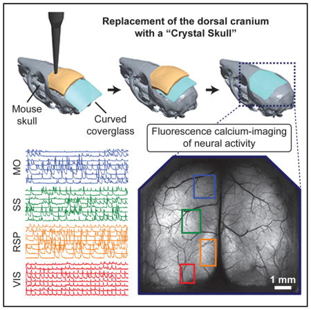
Kim et al. present a preparation for long-term imaging in which a curved glass window replaces the mouse dorsal cranium. This method enables large-scale Ca²⁺ imaging of neuronal dynamics across neocortex in behaving mice and yields an estimated >1 million optically accessible neurons by two-photon microscopy.

INTRODUCTION

Chronic preparations allowing long-term optical access to the live mammalian brain have greatly expanded our understanding of how the attributes of single neurons and neural ensembles relate to brain function. In mice, common methods for repeated imaging across weeks include glass cranial window (Goldey et al., 2014; Holtmaat et al., 2009), thinned skull, (Drew et al., 2010; Silasi et al., 2013; Yang et al., 2010), chemically induced cranial transparency (Silasi et al., 2016), and implanted microendoscope preparations (Barretto et al., 2011; Ziv et al., 2013). These approaches have allowed in vivo imaging studies of sub-cellular morphology (Attardo et al., 2015; Grutzendler et al., 2002; Trachtenberg et al., 2002), ensemble neural Ca²⁺ activity (Huber et al., 2012; Peters et al., 2014; Rubin et al., 2015), and aggregate neural activation (Murphy et al., 2016), as well as studies that combined optogenetics and in vivo imaging (Carrillo-Reid et al., 2016; Packer et al., 2015; Rickgauer et al., 2014).

In parallel to these advances, the aim of understanding how different brain areas interact has led to specialized microscopes that can concurrently monitor cells in two or more brain areas that are contiguous (Chen et al., 2016; Sofroniew et al., 2016; Stirman et al., 2016) or widely separated (Lecoq et al., 2014). For use with such instruments, existing preparations for long-term cellular-level imaging in mice make areas of brain tissue up to ~5 mm in diameter optically accessible (Holtmaat et al., 2009; Lecoq et al., 2014; Packer et al., 2015; Stirman et al., 2016; Wekselblatt et al., 2016).

A key technical goal has been to interrogate even broader portions of the mammalian brain at cellular and sub-cellular resolution. The advent of transgenic mice that in principle allow brain-wide studies of cellular morphology (Feng et al., 2000), ensemble neural Ca²⁺ activity (Dana et al., 2014; Madisen et al., 2015; Wekselblatt et al., 2016), or immediate early gene activation (Vousden et al., 2015) has made the development of chronic preparations and optical instruments with broader fields of view all the more pressing. Several advisory groups (Alivisatos et al., 2012, 2013) and the NIH BRAIN Initiative (BRAIN Initiative, 2014) have stressed the need to increase the number of individual cells whose dynamics can be monitored simultaneously in behaving mammals. By combining large-field, cranial viewing windows and future instruments for observing brain activity across multiple length scales, it might be possible to track the concurrent dynamics of hundreds of thousands to >1 million individual cells in active animals.

Here, we introduce a chronic mouse preparation that may help to reach this goal by allowing long-term optical access, at cellular and sub-cellular resolution, across the dorsal cortical surface. We term our preparation the “Crystal Skull,” and it is compatible with a variety of imaging and photo-stimulation modalities. After a single surgery, the preparation can provide access in awake mice to the Ca²⁺ activity of an estimated 25,000–50,000 cortical neurons via one-photon fluorescence imaging and an estimated >1 million neurons via two-photon imaging. It is not yet feasible to monitor all these cells individually at the same time. Nevertheless, that a single surgery affords access to this many individual cells provides compelling motivation to engineer instrumentation capable of neural recordings at a massive scale.

RESULTS

Curved Glass Replacement for the Dorsal Cranium

The central idea behind the Crystal Skull method is to cut and curve a microscope cover glass to match both the lateral extent and natural curvature of the mouse skull (Figure 1A). Unlike conventional cranial window methods, which use a flat cover glass, the curved window imparts far less mechanical compression to underlying tissue. Compression of brain tissue is relatively minimal with flat windows a few millimeters in diameter, but it becomes more substantial with larger windows. For example, a flat window over an 8-mm-diameter craniotomy compresses tissue at the center of the opening by ~0.8 mm perpendicular to the glass. The need to match the cranium’s natural curvature is especially important for windows encasing both cortical hemispheres; such windows unavoidably cover the major mid-line blood vessels (Figure 1B), and damage to these vessels can compromise brain health.

Figure 1. The Crystal Skull Preparation Allows Long-Term Optical Access across the Live Mouse Cortex with Minimal Inflammation.

(A) We made trapezoidal shaped windows from a standard (#0–#2) microscope cover glass (left). The resulting glass piece was heated and curved against a cylindrical mold (middle). The implant replaces the left and right parietal bones and parts of the frontal bone (right). Scale bar, 2 mm.

(B) The implant is stable for months after implantation. There is limited to no skull re-growth under the glass, making the method compatible with longitudinal studies. SSS, superior sagittal sinus. Scale bar, 1 mm.

(C) Histological analysis reveals comparable levels of cortical astrocytes in Crystal Skull mice as in mice that had no surgeries. We took tissue samples 2–5 weeks after surgery and stained them with DAPI, which labels nuclei of all cells (blue), and anti-glial fibrillary acidic protein (anti-GFAP; red). Scale bars represent 100 μm (top row) and 50 μm (bottom row).

See also Figures S1–S3 and Table S1.

Notably, the Crystal Skull technique is distinct from methods that involve thinning the skull over broad areas of the brain (Silasi et al., 2013), and there are key differences regarding the creation, optical quality, and stability of the resulting preparations. First, in our experience, it is faster and easier to replace the dorsal skull with glass than to try and thin uniformly the entire dorsal skull without rupturing it. Second, the optical quality of the Crystal Skull window is commercial optical grade; by comparison, the optical quality of a thinned skull preparation is limited by the intrinsic material variations and surface roughness of a thinned skull bone (Helm et al., 2009; Yang et al., 2010). Third, the Crystal Skull preparation is stable over months (Figure 1B), whereas skull re-growth generally alters the optical quality of a thinned skull preparation.

As the Crystal Skull involves a cranial replacement of unprecedented size in the mouse, requiring removal of most of the left and right parietal bones and a part of the frontal bone, we devised a way to minimize mechanical stress on the brain while installing the curved window (Experimental Procedures; Table S1; Figures S1 and S2). Our procedure seeks to minimize both compression and expansion of the brain (Figure S1). After implantation of the window, it usually remained clear for months, with negligible inflammation and skull re-growth (n = 18 mice; Figures 1B and 1C). In a subset of mice (n = 4), 2–5 weeks after surgery, we performed histological analyses to check for activated astrocytes by immunostaining for glial fibrillary acidic protein (GFAP). We chose GFAP due to its persistence at a glial scar for longer periods than a microglial marker such as CD68 (Attardo et al., 2015). These studies revealed comparable glial activation in cortical tissue from Crystal Skull mice and in control mice that had no surgeries (Figures 1C and S3). We also immunostained for NG2 glia and found comparable labeling patterns in both groups.

In Vivo Imaging of Neural Morphology across the Cortex

To verify that the preparation allowed sub-cellular resolution across cortex, we used two-photon microscopy to examine neural morphologies in anesthetized Thy1-YFP-H mice (Feng et al., 2000; Grutzendler et al., 2002), which express the yellow fluorescent protein (YFP) in a subset of layer 5 pyramidal cells (n = 3 mice). We acquired tiled series of three-dimensional image stacks arranged parallel to either the mediolateral or anterior-posterior axes (Figures 2A–2E). The images had sub-cellular resolution throughout (Figures 2B–2E), as illustrated by the apical dendrites seen across the 8.9-mm lateral span (Figures 2B and 2C). Using 20–50 mW of illumination delivered to the brain, pyramidal cell bodies were visible up to ~700 μm below the cortical surface, as were individual dendritic branches (Figure 2D). We attained comparable resolution and imaging depths across the glass window’s anterior-posterior span (Figure 2E).

Figure 2. The Crystal Skull allows In Vivo Imaging of Sub-cellular Features across Cortex.

(A) Epi-fluorescence image of a live Thy-1-YFP-H mouse, which expresses the yellow fluorescent protein (YFP) in a subset of layer 5 pyramidal neurons, with a Crystal Skull. Red and blue rectangles enclose regions shown in (B) and (E), respectively. Scale bar, 1 mm.

(B) A tiling of two-photon image-stacks (two-dimensional projections of three-dimensional image stacks) acquired in the live mouse of (A) within the corresponding red-boxed area, visualized as a coronal section (1.8 mm × 8.9 mm). Pyramidal cell bodies are visible up to ~700 μm beneath the cortical surface. Dashed green box indicates the region shown in panel (C). Scale bar, 1 mm.

(C) Magnified view of the green-boxed area in (B). Cell bodies and apical dendrites are visible ~300–700 μm beneath the cortical surface. Dashed yellow line marks the depth of the two-photon image shown in panel (D). Scale bar, 100 μm.

(D) Two-photon image of YFP-labeled cell bodies and dendrites, acquired ~350 μm from the cortical surface. Scale bar, 100 μm.

(E) A tiling of two-photon image-stacks (two-dimensional projections of three-dimensional image stacks) acquired in the live mouse of (A) within the corresponding blue-boxed area, visualized as a sagittal section (0.8 mm × 4.9 mm) Scale bar, 500 μm.

(F) Epi-fluorescence macroscope image of a live Thy-1-GFP-M mouse, which expresses GFP in a sparse subset of layer 5 pyramidal neurons, with a Crystal Skull. Circles indicate locations where we took the two-photon images of (G)–(I) (marked in color-corresponding outlines). Scale bar, 1 mm.

(G–I) Dendrites and dendritic spines imaged by two-photon microscopy in the areas enclosed in colored circles in (F). Scale bar, 10 μm.

Using a sparsely fluorescent mouse line (Thy-1-GFP-M) expressing GFP in a minority of layer 2/3 pyramidal cells (Feng et al., 2000), we performed high-magnification two-photon imaging of neural dendrites at multiple regions of interest (ROIs) across the Crystal Skull (n = 2 mice) (Figure 2F). Dendritic spines were readily discernible, as expected from prior in vivo imaging studies of these mice (Trachtenberg et al., 2002) (Figure 2G–2I).

Large-Scale Ca²⁺ Imaging in Awake Mice

We next evaluated our capacity to monitor neural activity across the dorsal cortex of behaving mice. We installed curved windows in GCaMP6f-tTA-dCre mice expressing the Ca²⁺-indicator GCaMP6f in layer 2/3 pyramidal cells (Madisen et al., 2015) and used a variable-zoom, low-magnification epi-fluorescence macroscope to visualize Ca²⁺ activity across the entirety of the Crystal Skull while the mice were head-fixed and awake (n = 7 mice). Although the objective lens (1.0× magnification) was not optimized for high-resolution imaging, we readily observed individual active neurons in multiple cortical areas (Figures 3A and 3B; Movies S1, S2, and S3). Due to the brain’s curvature, it was not possible to keep layer 2/3 in focus across the entire field of view; at a fixed focal setting, active cells were plainly apparent in some areas but out of focus in others (Movies S1 and S2).

Figure 3. An Estimated 25,000–50,000 GCaMP6f-Expressing Pyramidal Cells Are Optically Accessible through the Crystal Skull by One-Photon Ca²⁺ Imaging.

(A) A maximum projection image, computed across a 20-s recording of neural Ca²⁺ activity. The video recording was acquired on an epi-fluorescence macroscope and reveals individual cells across the dorsal cortex of a GCaMP6f-tTA-dCre triple-transgenic mouse expressing GCaMP6f in cortical layer 2/3 pyramidal cells. Color overlay atop the left hemisphere is based on the Allen Brain Atlas (Oh et al., 2014) and shows a sampling of the >30 cortical areas that are accessible. 18 areas in the left hemisphere are marked. CC, cingulate cortex; MOp, primary motor area; MOs, secondary motor area; SSp-bfd, primary somatosensory area (barrel field); SSp-m, primary somatosensory area (mouth); SSp-ul, primary somatosensory area (upper limb); SSp-ll, primary somatosensory area (lower limb); SSp-tr, primary somatosensory area (trunk); SSs, secondary motor area; AUD, auditory area; PTLp, posterior parietal association area; RSP, retrosplenial area; VISal, anterolateral visual area; VISam, anteromedial visual area; VISp, primary visual area; VISpm, posteromedial visual area; TEa, temporal association area; ECT, ectorhinal area.

Red box marks the area shown in (B) and used for computational sorting of cells based on their Ca²⁺ activity. Scale bar, 1 mm.

(B) Top: map of 1,166 cells in the red-boxed area in (A) and identified computationally in epi-fluorescence Ca²⁺ videos. Bottom: 30 example Ca²⁺ activity traces. Locations of individual cells are marked with corresponding numerals in the map. Scale bar, 100 μm.

(C) Trial structure of a simple behavioral protocol involving visual stimulation and reward delivery. At the start of each trial, the mouse saw five flashes of blue light (pulses 0.1 ms in duration, timed to start 0.2 ms apart) with its right eye. After a 1.7-s delay, the mouse received a water reward (~5–10 μL) from a spout. The inter-trial interval varied from 4 to 6 s.

(D) A maximum projection image of the dorsal cortex, computed across a 3.5-min recording of neural Ca²⁺ activity in a mouse undergoing the protocol of (C). Colored boxes indicate cortical areas (red, visual; orange, retrosplenial; green, somatosensory; blue, motor) where we acquired additional Ca²⁺ imaging data at a higher magnification for computational extraction of individual cells. During Ca²⁺ imaging in each of these four areas, the mouse performed 24 behavioral trials. Scale bar, 1 mm.

(E) Map of 262 cells in the red-boxed area in (D) (visual cortex) and identified computationally in epi-fluorescence Ca²⁺ videos as the mouse performed the protocol of (C). Activity traces for the numbered cells are shown in red in (G). Scale bar, 250 μm.

(F) Map of 420 cells in the green-boxed area in (D) (somatosensory cortex) and identified computationally in epi-fluorescence Ca²⁺ videos as the mouse performed the protocol of (C). Activity traces for the numbered cells are shown in green in (G). Scale bar, 250 μm.

(G) Left: example traces of neural Ca²⁺ activity acquired by epi-fluorescence imaging in the four color-corresponding areas in (D). The traces from visual and somatosensory cortex are those of the numbered cells in (E) and (F), respectively. Right: traces obtained by averaging each cell’s responses across all 24 trials. Yellow triangles mark the start of each trial. The blue triangle marks reward delivery.

Nonetheless, we could bring each visible brain area into focus simply by adjusting the focal plane. For example, in awake head-restrained GCaMP6f-tTA-dCre mice (n = 2) to which we presented sets of five visual flashes followed by water reward (Figure 3C; Supplemental Experimental Procedures), we used the macroscope to perform one-photon Ca²⁺ imaging in four distinct brain areas, with each area examined serially on each of four successive days (Figures 3D–3G). In these studies, many visual neurons exhibited Ca²⁺ activity time-locked to visual stimulation, and many somatosensory neurons activated at reward delivery, whereas cells in the retrosplenial and motor cortices had more heterogeneous responses (Figure 3G).

We estimated the total number of GCaMP6f-expressing cells that were identifiable by one-photon Ca²⁺ imaging. Using Ca²⁺ videos acquired in 1.3 × 1.3-mm² tissue areas (n = 4 GCaMP6f-tTA-dCre mice) (Movie S3), computational cell sorting identified up to 1,166 neurons per sample area (Figure 3B). The resulting estimated cellular densities, when scaled to the entire Crystal Skull, suggest that ~25,000–50,000 individual layer 2/3 neurons are available for one-photon Ca²⁺ imaging in this mouse line (Experimental Procedures).

As one-photon Ca²⁺ imaging is limited to ~150–200 μm depths into brain tissue (Hamel et al., 2015), we next used two-photon microscopy to study the GCaMP6f-tTa-dCre mice and also tetO-GCaMP6s/CaMK2a-tTA mice expressing the Ca²⁺ indicator GCaMP6s in a subset of pyramidal neurons (Figure 4) (Wekselblatt et al., 2016). Individual cells were visible across cortex in two-photon image mosaics and could be tracked over days (Figures 4A and 4B). To estimate the total number of GCaMP6s-expressing cells accessible by two-photon imaging, we randomly selected 460-μm × 460-μm regions of interest and monitored Ca²⁺ activity at a series of depths 100–500 μm below the cortical surface (n = 4 volumes sampled in 3 mice; Figures 4C and 4D; Movie S4). To identify individual cells and their activity traces in the resulting datasets, we performed computational cell sorting on the Ca²⁺ videos taken at each tissue depth (Experimental Procedures). This yielded high-fidelity activity traces from cells up to 500 μm beneath the glass window (Figures 4E–4G). We tallied the total number of active cells while ensuring that cells visible in axially adjacent image planes contributed only once to the count. The densities of cortical neurons identified by their Ca²⁺ activity were consistent with values found previously by two-photon Ca²⁺ imaging (Huber et al., 2012; Lecoq et al., 2014; Peters et al., 2014). When scaled to the area of the entire Crystal Skull, the tallies of active cells in GCaMP6s/CaMK2a-tTA mice imply that an estimated 0.8–1.1 million cortical neurons are accessible by in vivo two-photon Ca²⁺ imaging.

Figure 4. Two-Photon Microscopy Makes a Million or More Neurons Optically Accessible through the Crystal Skull and Allows Time-Lapse Imaging of Individual Cells.

(A) Mosaic of tiled two-photon images from the right hemisphere of a GCaMP6f-tTA-dCre mouse expressing GCaMP6f in cortical layer 2/3 pyramidal cells. Boundaries between tiles are apparent, because adjacent image tiles were acquired in different axial planes. The mouse is the same as in Figure 3A. Scale bar, 1 mm. Insets: magnified views of the color-corresponding boxed areas in the main panel. Scale bar, 100 μm (all insets).

(B) Time-lapse imaging of individual cells in a tetO-GCaMP6s/CaMK2a-tTA mouse, which expresses GCaMP6s in a subset of pyramidal neurons. Individual cells can be tracked for multiple days. The day of imaging is indicated in the lower left of each image, starting with the first session on day 1. Scale bar, 100 μm.

(C) Epi-fluorescence macroscope image of a tetO-GCaMP6s/CaMK2a-tTA mouse. Three regions of interest (ROIs) indicate locations where we took two-photon Ca²⁺ videos according to the protocol in (D) and at multiple tissue depths. Scale bar, 1 mm.

(D) Protocol for two-photon Ca²⁺ imaging at the three ROI locations marked in (C). Within each ROI, we acquired 5-min movies at each of a series of tissue depths 100–500 μm from the cortical surface and spaced 10–20 μm apart.

(E–G) Top: example cell maps determined by two-photon Ca²⁺ imaging in a tetO-GCaMP6s/CaMK2a-tTA mouse. Colors of the panel borders indicate the color-corresponding ROIs in (C). The tissue depth of each image is given above the panels. Bottom: for each panel, 15 Ca²⁺ activity traces are shown. Locations of individual cells are marked with numerals in the corresponding map. Scale bar, 100 μm.

DISCUSSION

By shaping optical-grade glass to mimic the curved form of the mouse skull and creating surgical methods to install this cranial replacement, we attained chronic optical access to individual cells across the dorsal cortex. The implant is stable for months (Figure 1B), and based on the Allen Mouse Brain Atlas (Oh et al., 2014), cells are visible across 30–40 brain areas. The access to individual cells is a crucial distinction from prior preparations in which the skull is thinned over the entire cranial surface or rendered transparent by chemical means, as these past methods have not enabled cellular imaging (Silasi et al., 2013, 2016). We estimated that 25,000–50,000 individual neurons are accessible per mouse using wide-field epi-fluorescence imaging, and >1 million active cells are accessible by two-photon microscopy.

Using a green fluorescent indicator and two-photon imaging, we tracked the Ca²⁺ dynamics of cells up to ~500 μm below the cortical surface; by using indicators with longer excitation wavelengths, even greater tissue depths and more cells will be accessible (Dana et al., 2016; Inoue et al., 2015). A range of imaging and optogenetic methods can be combined with the Crystal Skull preparation, which is also compatible with many different behavioral assays for head-fixed mice.

Implications for the Design of Brain Imaging Studies

Owing to its span across the cortex, the Crystal Skull may allow brain imaging or optogenetic studies that are more unbiased than those conducted to date. In past studies of cellular activity, researchers usually had to select one or a few brain areas at the outset of experimentation. However, neocortical areas share a complex web of connections, both direct and indirect, and it seems likely that the commonly studied behavioral assays engage brain areas well beyond those that have attracted the most research. A more unbiased approach using the Crystal Skull might help reduce the need to choose candidate brain areas for study based on previous knowledge.

Researchers using the Crystal Skull might identify brain areas of interest based on the empirically determined neural responses evoked by specific stimuli or behaviors. An individualized mode of study could take into account that different mice might have unique neural activity patterns meriting customized follow-up investigations. Future studies might seek to explain the differences between individual mice on the basis of their distinctive brain activity patterns. Aiding such an approach, the Crystal Skull might facilitate quantitative comparisons across multiple brain areas and tailoring of optical investigations to the dynamical patterns found in each animal.

Implications for Systems Neuroscience Research

Research advisory groups and the NIH have called for new technologies that can track the dynamics of >1 million individual neurons in behaving animals (Alivisatos et al., 2012, 2013; BRAIN Initiative, 2014). Candidate recording modalities with this capacity might use signals that are electrical, optical, or of another energy form. On its own, the Crystal Skull does not reach this milestone. However, the access it provides to >1 million active cells after one surgery suggests that a promising route to realizing massive recordings in the live brain may lie in the optical domain.

To make full use of the Crystal Skull preparation, researchers should engineer several types of new instrumentation. Our commercial epi-fluorescence macroscope cannot attain cellular resolution across the entire dorsal cortex, at high numerical aperture, in a single image frame. Surpassing this limitation might require superior wide-field optics, fast scientific-grade cameras of greater pixel counts, and means of sampling the entire depth of field of the curved cortical surface. Several fluorescence-imaging modalities with an extended depth of field already exist and show promise for further improvements (Broxton et al., 2013; Fahrbach et al., 2013; Prevedel et al., 2014; Quirin et al., 2014).

Similarly, extant two-photon microscopes can only sample a portion of the tissue volume that is accessible via the Crystal Skull unless a tiling strategy is used. Recent work has expanded the field of view that is addressable by laser-scanning two-photon microscopy (Chen et al., 2016; Lecoq et al., 2014; Sofroniew et al., 2016; Stirman et al., 2016), proposed new forms of scanless volumetric imaging (Prevedel et al., 2014; Watson et al., 2010), and demonstrated variants of two-photon imaging in which more than one illumination beam sweeps across brain tissue (Chen et al., 2016; Lecoq et al., 2014; Stirman et al., 2016). However, no microscope today comes close to being able to track simultaneously the million or more cells that the Crystal Skull makes available for long-term imaging in the adult mouse brain.

Although it is possible to envision advanced instrumentation for imaging across the Crystal Skull at cellular resolution, notable constraints come from the total energy and spatial distribution of illumination that the brain can safely tolerate (Marblestone et al., 2013). Perhaps equally vital as new instrumentation may be the development of fluorescent indicators of neural activity that provide high signal-detection fidelities while operating at weak illumination intensities. A fluorescent indicator’s absorption cross-section and molecular brightness are key parameters, but signal-detection theory also shows that indicators with ultra-low baseline emissions can enable high-fidelity detection with only modest emission intensities (Wilt et al., 2013). To design strategies for concurrent recordings of as many neurons as possible via the Crystal Skull, it may be necessary to take a holistic, systems engineering approach that optimizes the optical instrumentation and indicators jointly (BRAIN Initiative, 2014).

In the immediate future we expect that multiple strategies based on established optical techniques will make use of the new possibilities introduced here for imaging broad fields of view, relating observations across length scales from microns to millimeters, and studying interactions between tens of brain areas in behaving mice. Through longitudinal studies of both ensemble activity patterns and single cell properties, it should also be possible to examine the long-term dynamics of the brain’s network attributes in a multi-scale manner.

EXPERIMENTAL PROCEDURES

Mice

Stanford Administrative Panel on Laboratory Animal Care (APLAC) approved all animal procedures. We used Thy1-GFP-M mice (Jackson Laboratory, #007788), Thy1-YFP-H mice (Jackson Laboratory, #003782), double-transgenic tetO-GCaMP6s/CaMK2a-tTA mice (Tg(tetO-GCaMP6s)2Niell; Jackson Laboratory, #024742; B6.Cg-Tg(CaMK2a-tTA)1Mmay/DboJ; Jackson Laboratory, #007004) and triple transgenic GCaMP6f-tTA-dCre mice from the Allen Institute (Rasgrf2-2A-dCre/CaMK2a-tTA/Ai93). Mice were 10–16 weeks old at the time of surgery and resided in a reverse-light-cycle facility.

Curved Glass Windows

We designed trapezoidal shapes in optical-grade glass stock (0.2–0.3 mm thickness; Schott, D263T) and had them commercially cut (TLC International) and bent to a desired curvature by heating and pressing against a cylindrical graphite mold (GlasWerk) (Figure 1A). We cleaned curved glass pieces in soap and water in an ultrasonicator and then washed and stored them in ethanol prior to surgical implantation.

Surgery

Step-by-step instructions for installing the Crystal Skull implant are listed in Table S1. We anesthetized mice with isoflurane (4% for induction and 1%–2% during surgery). To minimize inflammation and brain edema, we injected carprofen (5–10 mg/kg) and dexamethasone (2 mg/kg) subcutaneously prior to surgical incision. We applied ointment to the mouse’s eyes to maintain their moisture. A heating pad (FHC, 40-90-8D) maintained the mouse’s body temperature at 37°C.

We removed the skin atop the cranium and cleaned the skull surface with a scalpel while continuously perfusing mammalian Ringer’s solution (Electron Microscopy Science, #11763-10) over the surgical area. Next, we performed a craniotomy matched in size and shape to the outline of the trapezoidal glass implant (Figures 1A and S1). To make the craniotomy, we first created a shallow groove along the perimeter of the trapezoid using a 0.7-mm-diameter drill (Fine Science Tools, 19007-07). We used a 0.5-mm-diameter drill (Fine Science Tools, 19007-05) to deepen the groove and disconnect the trapezoidal-shaped bone piece from the surrounding skull. We perfused mammalian Ringer’s solution throughout the drilling. Once the bone piece was disconnected from the skull, we pressed down gently on its anterior edge to elevate its posterior end (Figure S1B). We slid the glass window underneath the elevated bone piece while taking care to avoid scraping the brain surface. When approximately two-thirds of the glass was inserted, we removed the overlying bone piece with forceps while continuing to position the glass implant. We performed all steps under continuous perfusion of Ringer’s solution. We left the dura intact.

Once the Crystal Skull implant was in its final position, we dried its edges with surgical eye spears (Butler Schein Animal Health, #1556455) and glued the window to the skull with UV-light-cured adhesive (UV glue; Loctite, 4305). To allow head fixation during optical brain imaging, we installed a stainless steel annular head plate (12 mm inner diameter) (Figure S2A). We set the head plate around the glass window and filled the gap between the head plate and the skull with UV glue. After curing the glue, we cleaned the surface of the window and covered it with a hemispherical protective cap printed in plastic (Figure S2B). We transferred the mouse to a recovery cage and placed it on a heating pad until it awoke. We then returned the mouse to its home cage and provided food and water on the cage floor without use of a food hopper, which might have disturbed the protective cap. We subcutaneously administered the mice carprofen (5–10 mg/kg) for the first 3 days after surgery. For the first 7 days after surgery, we checked all mice daily for signs of distress. We resumed feeding using a food hopper 14 days after surgery.

In Vivo Brain Imaging

We acquired all two-photon fluorescence images using a commercial microscope (Bruker, Ultima). A Ti:sapphire laser (Spectra Physics, Mai Tai BB) provided ultrashort-pulsed illumination (920 nm center wavelength). We used a 20× 0.95 numerical aperture (NA) water-immersion objective lens (Olympus, XLUMPlanFL N) in all cases, except for acquisition of the three-dimensional image stacks taken along the medio-lateral axis (Figure 2B), for which we used a 16× 0.80 NA water-immersion lens (Nikon, CFI75 LWD 16xW). Mean illumination power delivered to the brain was 20–50 mW, depending on the depth in tissue of the focal plane. We detected fluorescence signals (500- to 550-nm wavelengths) using a band-pass filter (Chroma, ET525/50m-2p) and a GaAsP photomultiplier tube (Hamamatsu, H10770PA-40). All images had 512 × 512 pixels.

To acquire images of neural morphology (Figure 2), we anesthetized mice with isoflurane (4% induction, 1%–2% during imaging) and head-fixed them under the microscope objective lens using the head-plate implanted during surgery. We applied eye ointment and maintained body temperature at 36°C. We acquired tiled sets of three-dimensional image stacks parallel to the medio-lateral (ML) or anterior-posterior (AP) axes (Figure 2A). Along the ML direction (Figure 2B) we took 17 image stacks, with adjacent stacks spaced 500 μm apart, using the 16× 0.80 NA objective lens. Along the AP direction (Figure 2E), we took 12 image stacks, with the stacks spaced 400 μm apart, using the 20× 0.95 NA objective lens. The separations between adjacent stacks were less than the widths of the individual field-of-views (660 μm with the 16× objective and 460 μm with the 20× lens); thus, we achieved full coverage of the sampled tissue volumes (red and blue dashed boxes in Figure 2A). After locating the brain surface we acquired a stack of two-photon images starting from the pia and extending 500–800 μm into tissue. All stacks had 2 μm axial spacing between adjacent images.

To acquire two-photon Ca²⁺ videos in awake mice, we head-fixed them under the microscope objective lens using their implanted head plate; the mice could walk or run in place on a 11.4-mm-diameter Styrofoam ball (Plasteel) with two rotational degrees of freedom. We took all two-photon Ca²⁺ videos over a 460-μm × 460-μm field of view at a 1.5-Hz frame rate with the 20× 0.95 NA objective. We sampled columnar tissue volumes (Figure 4D) by acquiring 500 image frames at each axial depth, starting 100 μm below the pial surface and extending in increments of 10–20 μm to 500 μm below the surface.

We acquired epi-fluorescence images on a variable zoom macroscope (Leica, MZFL III) with a plan 1.0× objective lens (Leica, 10445819) and an sCMOS camera (Andor, Zyla). For Ca²⁺ imaging, we used a filter set designed for GFP (Leica, 10450756). A solid-state white light engine (Lumencor, Sola SM 5-LCR-VA) coupled to a 3-mm-diameter liquid light guide provided ~50 mW of illumination across a ~10-mm-diameter area. We head-fixed mice by their head plate under the objective lens; the mice could walk or run at liberty on a wheel (Innovive, Innowheel). The macroscope had a field of view (FOV) of 8 mm × 11 mm at a 1.3× zoom setting, sufficient to image the entire Crystal Skull implant (Movie S1). Alternatively, we used a 4-mm × 5-mm FOV at a zoom setting of 3.2× (Movie S2). We acquired Ca²⁺ videos used for extraction of individual cells at a 9.5-Hz frame rate. Over recording durations of <5 min, we observed no bleaching or signs of photodamage.

Mouse Behavior

During epi-fluorescence imaging of neural Ca²⁺ activity, each trial of the behavioral protocol began with five flashes of blue light (pulses 0.1 ms in duration, timed to begin 0.2 ms apart) visible to the mouse’s right eye. After a 1.7-s delay, the mouse then received a water reward. The inter-trial interval varied between 4 and 6 s.

On the first day of imaging, we monitored Ca²⁺ activity at a low optical magnification across the cortex for four periods of 3.5 min each. On the next three consecutive days, we imaged neural Ca²⁺ activity in each of four, successively examined cortical regions of interest (Figure 3D). The mouse performed 24–26 behavioral trials during examination of each of these areas. Figure 3D is from the first day of imaging, and Figures 3E–3G are from the third day. Supplemental Experimental Procedures has details of the behavioral setup and training.

Mosaic Images of Neural Morphology

Supplemental Experimental Procedures has details of how we computationally tiled images from across the cortex (Figures 2B and 2E).

Computational Identification of Individual Cells

To extract cells and their activity traces from the Ca²⁺ movies, we first corrected for brain motion by using the TurboReg algorithm to perform rigid image displacements and rotations (Thévenaz et al., 1998). To sort cells from one-photon Ca²⁺ videos, we used a method based on maximum likelihood maximization (Deneux et al., 2016; Harris et al., 2016). To sort cells from two-photon Ca²⁺ movies, we used the constrained non-negative matrix factorization (CNMF) cell-sorting algorithm (Pnevmatikakis et al., 2016). Outlines of the cells shown in Figures 3B, 3E, 3F, and Figures 4E–4G were computed as the contours at which each cell’s computationally determined spatial filter declined to 30% of its peak value. See Supplemental Experimental Procedures for details.

Estimates of Optically Accessible Active Cells

As it was not practical to sample all the cortical volume under the Crystal Skull at high resolution, we computed the total number of cells that were accessible via one- and two-photon imaging by determining the cell density in several randomly chosen ROIs and then using these values to estimate the total number of accessible cells over the 73.75 mm² Crystal Skull window (Figure 1A).

For one-photon Ca²⁺ imaging, we made estimates in four mice and extracted 1,166 cells in a 1.3-mm × 1.3-mm area (Figure 3B), 708 cells in a 1.3-mm × 1.3-mm area, 447 cells in a 1.5-mm × 0.85-mm area, and 769 cells in a 1.35-mm × 1.05-mm area. These values yielded estimates of 26,000–51,000 total accessible cells.

To estimate the number of cells accessible by two-photon imaging, using a common sampling protocol (Figure 4D) we sampled four separate volumes of interest, each with a 460-μm × 460-μm cross-section and axial planes spaced 10.5–12.5 μm apart, in three different mice. These volumes yielded 3,243 active cells (blue ROI in Figure 4C; 38 imaging planes), 2,939 active cells (green ROI in Figure 4C; 35 imaging planes), 3,000 active cells (32 planes), and 3,103 active cells (28 planes). These values project to 1.02–1.13 million accessible neurons across the Crystal Skull. A fifth volume, which we sampled at lower density with the axial planes spaced 20 μm apart (red ROI in Figure 4C; 20 planes), yielded an estimate of 804,000 total accessible cells. In making these estimates, we ensured that individual cells visible in axially adjacent image planes contributed only once to our tallies. To do this, we created for each cell in every plane a binary mask, attained by thresholding the cell’s spatial filter at 30% of its peak intensity. Then, for every pair of cells identified in axially adjacent planes, we defined an overlap score as the area of intersection of the two cells’ masks, divided by the area of the union of the two masks. We identified candidate cell pairs as two images of the same cell when the overlap score was >0.5.

Histological Analysis

See Supplemental Experimental Procedures.

Supplementary Material

Movie S1

Table S1. Surgical protocol for installing the Crystal Skull, Related to Figure 1.

Figure S1. Maintenance of normal pressure levels on the brain is a key aspect of installing the Crystal Skull, Related to Figure 1.

(A) We created a single craniotomy on the mouse skull along a trapezoidal outline. The central piece (trapezoidal area shown in yellow) is disconnected from the rest of the cranium.

(B) By pressing down gently on the anterior edge of the loose skull piece, we lift up its posterior end, thereby creating a gap between the skull and the surface of the brain.

(C) We slide the Crystal Skull implant (cyan) underneath the loose bone from its posterior end, with a slight upward tilt of the glass to avoid scraping the surface of the brain. The interface between the glass and the brain is lubricated with mammalian Ringer’s solution throughout.

(D) Once about two-thirds of the implant is inserted, we detach the loose skull with fine forceps. We continue to slide the Crystal Skull implant forward, moving it into its final position.

(E) Once the implant is in position, we dry the edges of the glass and the nearby skull with surgical eye spears. The implant is affixed to the skull using ultraviolet-light-cured optical glue.

Figure S2. A custom stainless steel head-plate surrounds the Crystal Skull and protects the glass implant when it is not in use for imaging, Related to Figure 1.

(A) In addition to the Crystal Skull optical implant, we mount a custom, 1.5-mm-thick stainless steel head-plate that allows head-fixation of the mouse. The head-plate has two threaded screw holes for mounting auxiliary apparatus to the head.

(B) We use a custom, 3D-printed plastic cap to protect the large window when optical access is not needed (e.g. when the animal is resting in its home cage).

Figure S3. Histologic analysis reveals minuscule levels of astrocytic activation in the neocortex of Crystal Skull mice, Related to Figure 1.

(A–E) Immunohistological analysis revealed comparable levels of neocortical astrocytes in Crystal Skull mice as in negative control mice (Figure 1C) that had no surgeries. We took brain tissue samples 2–5 weeks after surgery and stained them with DAPI, which labels the nuclei of all cells (blue), and anti-glial fibrillary acidic protein (anti-GFAP; red). Images are of five randomly selected neocortical tissue sites in a GCaMP6f-tTA-dCre mouse with a Crystal Skull. Images in the middle and right columns are shown at a higher magnification than images in the left column. Images in the right column also show the green fluorescence from GCaMP6f. Scale bars are 50 μm in the middle and right columns and 100 μm in the left column.

(F) Coronal section maps, based on those in (Paxinos and Franklin, 2012), show the approximate locations of the tissue samples in A–E.

(G, H) Brain tissue samples, stained with DAPI and anti-GFAP, from a positive control mouse, G, in which we deliberately nicked the brain during surgery to cause tissue damage, and a negative control mouse, H, that had no surgeries and for which the tissue sample underwent the immunostaining protocol but with the primary antibody deliberately withheld. For both G and H the scale bars are 200 μm (left panels) and 50 μm (right panels).

Supplemental Movie 1. Epi-fluorescence Ca²⁺ imaging through the Crystal Skull across the cortex of a GCaMP6f-tTA-dCre transgenic mouse reveals neuropil and single cell Ca²⁺ activity. Note that due to the curvature of the brain, it was not possible to focus upon cortical layer 2/3 simultaneously across all of neocortex. Hence, active neurons are apparent in some cortical regions, but other regions are out-of-focus and appear blurrier. Playback speed is 10× real-time. The video was taken 8 weeks after implantation of the curved glass window. Scale bar: 1 mm.

Movie S2. Supplemental Movie 2.

Epi-fluorescence Ca²⁺ imaging through the Crystal Skull over the retrospenial area of a GCaMP6f-tTA-dCre transgenic mouse reveals both neuropil and single cell Ca²⁺ activity. As this video has a higher magnification than Movie 1, a higher density of neurons is visible than in the lower magnification recording. Due to the curvature of the brain, it was not possible to focus upon cortical layer 2/3 simultaneously across all of the tissue shown. Hence, active neurons are apparent in some areas, but other areas are out-of-focus and appear blurrier. Playback speed is 10× real-time. The video was taken 8 weeks after implantation of the curved glass window. Scale bar: 0.5 mm.

Movie S3. Supplemental Movie 3.

An epi-fluorescence video of Ca²⁺ activity in the same mouse as in Movie 2, but acquired three weeks after Movie 2, at 11 weeks after implantation of the curved glass window. Left, Raw epi-fluorescence Ca²⁺ video data across a field of view approximately 4 mm × 3 mm in size. The square box encloses the 1.3 mm × 1.3 mm sub-region shown in the right panel. Scale bar is 0.5 mm. Right, Video of the relative changes in fluorescence (ΔF/F) across the boxed region of the left panel, highlighting the somatic Ca²⁺ activity of single neurons. Playback speed is 3× real-time.

Movie S4. Supplemental Movie 4.

Two-photon Ca²⁺ imaging through the Crystal Skull in a tetO-GCaMP6s/CaMK2a-ttA transgenic mouse, from the red region-of-interest marked in Figure 4C. From left to right, the individual Ca²⁺ videos were acquired at 100 μm, 200 μm and 350 μm beneath the cortical surface. Playback speed is 6× real-time. Scale bar: 100 μm.

Highlights.

• In the “Crystal Skull,” a curved glass window replaces the mouse’s dorsal cranium

• Long-term optical access to 30–40 neocortical brain areas in behaving mice

• Cellular- and sub-cellular-level resolution of neural morphology across the cortex

• Large-scale imaging reveals neural Ca²⁺ dynamics across cortex in active mice

References

- Alivisatos AP, Chun M, Church GM, Greenspan RJ, Roukes ML, Yuste R. The brain activity map project and the challenge of functional connectomics. Neuron. 2012;74:970–974. doi: 10.1016/j.neuron.2012.06.006. [DOI] [PMC free article] [PubMed] [Google Scholar]
- Alivisatos AP, Chun M, Church GM, Deisseroth K, Donoghue JP, Green-span RJ, McEuen PL, Roukes ML, Sejnowski TJ, Weiss PS, Yuste R. Neuroscience. The brain activity map Science. 2013;339:1284–1285. doi: 10.1126/science.1236939. [DOI] [PMC free article] [PubMed] [Google Scholar]
- Attardo A, Fitzgerald JE, Schnitzer MJ. Impermanence of dendritic spines in live adult CA1 hippocampus. Nature. 2015;523:592–596. doi: 10.1038/nature14467. [DOI] [PMC free article] [PubMed] [Google Scholar]
- Barretto RP, Ko TH, Jung JC, Wang TJ, Capps G, Waters AC, Ziv Y, Attardo A, Recht L, Schnitzer MJ. Time-lapse imaging of disease progression in deep brain areas using fluorescence microendoscopy. Nat Med. 2011;17:223–228. doi: 10.1038/nm.2292. [DOI] [PMC free article] [PubMed] [Google Scholar]
- BRAIN Initiative. BRAIN 2025: A Scientific Vision. U.S. Department of Health and Human Services (HHS); 2014. http://www.braininitiative.nih.gov/2025/index.htm. [Google Scholar]
- Broxton M, Grosenick L, Yang S, Cohen N, Andalman A, Deisseroth K, Levoy M. Wave optics theory and 3-D deconvolution for the light field microscope. Opt Express. 2013;21:25418–25439. doi: 10.1364/OE.21.025418. [DOI] [PMC free article] [PubMed] [Google Scholar]
- Carrillo-Reid L, Yang W, Bando Y, Peterka DS, Yuste R. Imprinting and recalling cortical ensembles. Science. 2016;353:691–694. doi: 10.1126/science.aaf7560. [DOI] [PMC free article] [PubMed] [Google Scholar]
- Chen JL, Voigt FF, Javadzadeh M, Krueppel R, Helmchen F. Long-range population dynamics of anatomically defined neocortical networks. eLife. 2016;5:e14679. doi: 10.7554/eLife.14679. [DOI] [PMC free article] [PubMed] [Google Scholar]
- Dana H, Chen TW, Hu A, Shields BC, Guo C, Looger LL, Kim DS, Svoboda K. Thy1-GCaMP6 transgenic mice for neuronal population imaging in vivo. PLoS ONE. 2014;9:e108697. doi: 10.1371/journal.pone.0108697. [DOI] [PMC free article] [PubMed] [Google Scholar]
- Dana H, Mohar B, Sun Y, Narayan S, Gordus A, Hasseman JP, Tsegaye G, Holt GT, Hu A, Walpita D, et al. Sensitive red protein calcium indicators for imaging neural activity. eLife. 2016;5:5. doi: 10.7554/eLife.12727. [DOI] [PMC free article] [PubMed] [Google Scholar]
- Deneux T, Kaszas A, Szalay G, Katona G, Lakner T, Grinvald A, Rózsa B, Vanzetta I. Accurate spike estimation from noisy calcium signals for ultrafast three-dimensional imaging of large neuronal populations in vivo. Nat Commun. 2016;7:12190. doi: 10.1038/ncomms12190. [DOI] [PMC free article] [PubMed] [Google Scholar]
- Drew PJ, Shih AY, Driscoll JD, Knutsen PM, Blinder P, Davalos D, Akassoglou K, Tsai PS, Kleinfeld D. Chronic optical access through a polished and reinforced thinned skull. Nat Methods. 2010;7:981–984. doi: 10.1038/nmeth.1530. [DOI] [PMC free article] [PubMed] [Google Scholar]
- Fahrbach FO, Voigt FF, Schmid B, Helmchen F, Huisken J. Rapid 3D light-sheet microscopy with a tunable lens. Opt Express. 2013;21:21010–21026. doi: 10.1364/OE.21.021010. [DOI] [PubMed] [Google Scholar]
- Feng G, Mellor RH, Bernstein M, Keller-Peck C, Nguyen QT, Wallace M, Nerbonne JM, Lichtman JW, Sanes JR. Imaging neuronal subsets in transgenic mice expressing multiple spectral variants of GFP. Neuron. 2000;28:41–51. doi: 10.1016/s0896-6273(00)00084-2. [DOI] [PubMed] [Google Scholar]
- Goldey GJ, Roumis DK, Glickfeld LL, Kerlin AM, Reid RC, Bonin V, Schafer DP, Andermann ML. Removable cranial windows for long-term imaging in awake mice. Nat Protoc. 2014;9:2515–2538. doi: 10.1038/nprot.2014.165. [DOI] [PMC free article] [PubMed] [Google Scholar]
- Grutzendler J, Kasthuri N, Gan WB. Long-term dendritic spine stability in the adult cortex. Nature. 2002;420:812–816. doi: 10.1038/nature01276. [DOI] [PubMed] [Google Scholar]
- Hamel EJ, Grewe BF, Parker JG, Schnitzer MJ. Cellular level brain imaging in behaving mammals: an engineering approach. Neuron. 2015;86:140–159. doi: 10.1016/j.neuron.2015.03.055. [DOI] [PMC free article] [PubMed] [Google Scholar]
- Harris KD, Quiroga RQ, Freeman J, Smith SL. Improving data quality in neuronal population recordings. Nat Neurosci. 2016;19:1165–1174. doi: 10.1038/nn.4365. [DOI] [PMC free article] [PubMed] [Google Scholar]
- Helm PJ, Ottersen OP, Nase G. Analysis of optical properties of the mouse cranium–implications for in vivo multi photon laser scanning microscopy. J Neurosci Methods. 2009;178:316–322. doi: 10.1016/j.jneumeth.2008.12.032. [DOI] [PubMed] [Google Scholar]
- Holtmaat A, Bonhoeffer T, Chow DK, Chuckowree J, De Paola V, Hofer SB, Hübener M, Keck T, Knott G, Lee WCA, et al. Long-term, high-resolution imaging in the mouse neocortex through a chronic cranial window. Nat Protoc. 2009;4:1128–1144. doi: 10.1038/nprot.2009.89. [DOI] [PMC free article] [PubMed] [Google Scholar]
- Huber D, Gutnisky DA, Peron S, O’Connor DH, Wiegert JS, Tian L, Oertner TG, Looger LL, Svoboda K. Multiple dynamic representations in the motor cortex during sensorimotor learning. Nature. 2012;484:473–478. doi: 10.1038/nature11039. [DOI] [PMC free article] [PubMed] [Google Scholar]
- Inoue M, Takeuchi A, Horigane S, Ohkura M, Gengyo-Ando K, Fujii H, Kamijo S, Takemoto-Kimura S, Kano M, Nakai J, et al. Rational design of a high-affinity, fast, red calcium indicator R-CaMP2. Nat Methods. 2015;12:64–70. doi: 10.1038/nmeth.3185. [DOI] [PubMed] [Google Scholar]
- Lecoq J, Savall J, Vučinić D, Grewe BF, Kim H, Li JZ, Kitch LJ, Schnitzer MJ. Visualizing mammalian brain area interactions by dual-axis two-photon calcium imaging. Nat Neurosci. 2014;17:1825–1829. doi: 10.1038/nn.3867. [DOI] [PMC free article] [PubMed] [Google Scholar]
- Madisen L, Garner AR, Shimaoka D, Chuong AS, Klapoetke NC, Li L, van der Bourg A, Niino Y, Egolf L, Monetti C, et al. Transgenic mice for intersectional targeting of neural sensors and effectors with high specificity and performance. Neuron. 2015;85:942–958. doi: 10.1016/j.neuron.2015.02.022. [DOI] [PMC free article] [PubMed] [Google Scholar]
- Marblestone AH, Zamft BM, Maguire YG, Shapiro MG, Cybulski TR, Glaser JI, Amodei D, Stranges PB, Kalhor R, Dalrymple DA, et al. Physical principles for scalable neural recording. Front Comput Neurosci. 2013;7:137. doi: 10.3389/fncom.2013.00137. [DOI] [PMC free article] [PubMed] [Google Scholar]
- Murphy TH, Boyd JD, Bolaños F, Vanni MP, Silasi G, Haupt D, LeDue JM. High-throughput automated home-cage mesoscopic functional imaging of mouse cortex. Nat Commun. 2016;7:11611. doi: 10.1038/ncomms11611. [DOI] [PMC free article] [PubMed] [Google Scholar]
- Oh SW, Harris JA, Ng L, Winslow B, Cain N, Mihalas S, Wang Q, Lau C, Kuan L, Henry AM, et al. A mesoscale connectome of the mouse brain. Nature. 2014;508:207–214. doi: 10.1038/nature13186. [DOI] [PMC free article] [PubMed] [Google Scholar]
- Packer AM, Russell LE, Dalgleish HW, Häusser M. Simultaneous all-optical manipulation and recording of neural circuit activity with cellular resolution in vivo. Nat Methods. 2015;12:140–146. doi: 10.1038/nmeth.3217. [DOI] [PMC free article] [PubMed] [Google Scholar]
- Peters AJ, Chen SX, Komiyama T. Emergence of reproducible spatiotemporal activity during motor learning. Nature. 2014;510:263–267. doi: 10.1038/nature13235. [DOI] [PubMed] [Google Scholar]
- Pnevmatikakis EA, Soudry D, Gao Y, Machado TA, Merel J, Pfau D, Reardon T, Mu Y, Lacefield C, Yang W, et al. Simultaneous denoising, deconvolution, and demixing of calcium imaging data. Neuron. 2016;89:285–299. doi: 10.1016/j.neuron.2015.11.037. [DOI] [PMC free article] [PubMed] [Google Scholar]
- Prevedel R, Yoon YG, Hoffmann M, Pak N, Wetzstein G, Kato S, Schrödel T, Raskar R, Zimmer M, Boyden ES, Vaziri A. Simultaneous whole-animal 3D imaging of neuronal activity using light-field microscopy. Nat Methods. 2014;11:727–730. doi: 10.1038/nmeth.2964. [DOI] [PMC free article] [PubMed] [Google Scholar]
- Quirin S, Jackson J, Peterka DS, Yuste R. Simultaneous imaging of neural activity in three dimensions. Front Neural Circuits. 2014;8:29. doi: 10.3389/fncir.2014.00029. [DOI] [PMC free article] [PubMed] [Google Scholar]
- Rickgauer JP, Deisseroth K, Tank DW. Simultaneous cellular-resolution optical perturbation and imaging of place cell firing fields. Nat Neurosci. 2014;17:1816–1824. doi: 10.1038/nn.3866. [DOI] [PMC free article] [PubMed] [Google Scholar]
- Rubin A, Geva N, Sheintuch L, Ziv Y. Hippocampal ensemble dynamics timestamp events in long-term memory. eLife. 2015;4:4. doi: 10.7554/eLife.12247. [DOI] [PMC free article] [PubMed] [Google Scholar]
- Silasi G, Boyd JD, Ledue J, Murphy TH. Improved methods for chronic light-based motor mapping in mice: automated movement tracking with accelerometers, and chronic EEG recording in a bilateral thin-skull preparation. Front Neural Circuits. 2013;7:123. doi: 10.3389/fncir.2013.00123. [DOI] [PMC free article] [PubMed] [Google Scholar]
- Silasi G, Xiao D, Vanni MP, Chen AC, Murphy TH. Intact skull chronic windows for mesoscopic wide-field imaging in awake mice. J Neurosci Methods. 2016;267:141–149. doi: 10.1016/j.jneumeth.2016.04.012. [DOI] [PMC free article] [PubMed] [Google Scholar]
- Sofroniew NJ, Flickinger D, King J, Svoboda K. A large field of view two-photon mesoscope with subcellular resolution for in vivo imaging. eLife. 2016;5:e14472. doi: 10.7554/eLife.14472. [DOI] [PMC free article] [PubMed] [Google Scholar]
- Stirman JN, Smith IT, Kudenov MW, Smith SL. Wide field-of-view, multi-region, two-photon imaging of neuronal activity in the mammalian brain. Nat Biotechnol. 2016;34:857–862. doi: 10.1038/nbt.3594. [DOI] [PMC free article] [PubMed] [Google Scholar]
- Thévenaz P, Ruttimann UE, Unser M. A pyramid approach to subpixel registration based on intensity. IEEE Trans Image Process. 1998;7:27–41. doi: 10.1109/83.650848. [DOI] [PubMed] [Google Scholar]
- Trachtenberg JT, Chen BE, Knott GW, Feng G, Sanes JR, Welker E, Svoboda K. Long-term in vivo imaging of experience-dependent synaptic plasticity in adult cortex. Nature. 2002;420:788–794. doi: 10.1038/nature01273. [DOI] [PubMed] [Google Scholar]
- Vousden DA, Epp J, Okuno H, Nieman BJ, van Eede M, Dazai J, Ragan T, Bito H, Frankland PW, Lerch JP, Henkelman RM. Whole-brain mapping of behaviourally induced neural activation in mice. Brain Struct Funct. 2015;220:2043–2057. doi: 10.1007/s00429-014-0774-0. [DOI] [PubMed] [Google Scholar]
- Watson BO, Nikolenko V, Araya R, Peterka DS, Woodruff A, Yuste R. Two-photon microscopy with diffractive optical elements and spatial light modulators. Front Neurosci. 2010;4:29. doi: 10.3389/fnins.2010.00029. [DOI] [PMC free article] [PubMed] [Google Scholar]
- Wekselblatt JB, Flister ED, Piscopo DM, Niell CM. Large-scale imaging of cortical dynamics during sensory perception and behavior. J Neurophysiol. 2016;115:2852–2866. doi: 10.1152/jn.01056.2015. [DOI] [PMC free article] [PubMed] [Google Scholar]
- Wilt BA, Fitzgerald JE, Schnitzer MJ. Photon shot noise limits on optical detection of neuronal spikes and estimation of spike timing. Biophys J. 2013;104:51–62. doi: 10.1016/j.bpj.2012.07.058. [DOI] [PMC free article] [PubMed] [Google Scholar]
- Yang G, Pan F, Parkhurst CN, Grutzendler J, Gan WB. Thinned-skull cranial window technique for long-term imaging of the cortex in live mice. Nat Protoc. 2010;5:201–208. doi: 10.1038/nprot.2009.222. [DOI] [PMC free article] [PubMed] [Google Scholar]
- Ziv Y, Burns LD, Cocker ED, Hamel EO, Ghosh KK, Kitch LJ, El Gamal A, Schnitzer MJ. Long-term dynamics of CA1 hippocampal place codes. Nat Neurosci. 2013;16:264–266. doi: 10.1038/nn.3329. [DOI] [PMC free article] [PubMed] [Google Scholar]
Associated Data
This section collects any data citations, data availability statements, or supplementary materials included in this article.
Supplementary Materials