Abstract
Markov state models (MSMs) and other related kinetic network models are frequently used to study the long-timescale dynamical behavior of biomolecular and materials systems. MSMs are often constructed bottom-up using brute-force molecular dynamics (MD) simulations when the model contains a large number of states and kinetic pathways that are not known a priori. However, the resulting network generally encompasses only parts of the configurational space, and regardless of any additional MD performed, several states and pathways will still remain missing. This implies that the duration for which the MSM can faithfully capture the true dynamics, which we term as the validity time for the MSM, is always finite and unfortunately much shorter than the MD time invested to construct the model. A general framework that relates the kinetic uncertainty in the model to the validity time, missing states and pathways, network topology, and statistical sampling is presented. Performing additional calculations for frequently-sampled states/pathways may not alter the MSM validity time. A new class of enhanced kinetic sampling techniques is introduced that aims at targeting rare states/pathways that contribute most to the uncertainty so that the validity time is boosted in an effective manner. Examples including straightforward 1D energy landscapes, lattice models, and biomolecular systems are provided to illustrate the application of the method. Developments presented here will be of interest to the kinetic Monte Carlo community as well.
I. INTRODUCTION
Recent years have witnessed the widespread use of Markov state models (MSMs)1–5 within the biophysics community. MSMs are detailed kinetic network models wherein the configurational space of a biomolecule under study is partitioned into states. The dynamical evolution of the system is approximated in terms of state-to-state transitions. The number of states can range between tens to thousands depending on the complexity and level of coarse-graining. Each node in the network denotes a metastable state of the system while the connections between the nodes provide rates of interconversion between the states. MSMs have become useful tools for probing the dynamics of nucleic acids and proteins,6–9 e.g., folding and unfolding events at long time scales. Though we restrict ourselves to biomolecular systems, MSMs are closely related to kinetic Monte Carlo (KMC) models10–12 used in the materials and reactions areas for studying catalysis,13 crystal growth,14 material processing,15 and adsorption phenomena16 to name a few. Both approaches solve a master equation and have benefitted from the exchange of ideas between the respective communities. For instance, knowledge of the network structure can be exploited to accelerate the KMC dynamics by eliminating fast degrees of freedom.17–20 Despite their widespread usage, some aspects of MSM construction are still poorly understood.
A key step in the MSM construction entails determining states and kinetic pathways to be included in the model. The availability of a large number of parallel processors has enabled rapid construction of high fidelity MSMs using brute-force molecular dynamics (MD) calculations.21–23 Herein states and kinetic pathways are identified via coarse-graining several independent MD trajectories. The MD trajectories can be seeded from different starting configurations, which allows for better sampling of the configurational space. Other simulation techniques offering resolution greater than the MSMs can also be employed.24–26 Enhanced thermodynamic-sampling techniques that can sample rare events with large energy barriers can aid in the efficient construction of the model.27–31 However, often overlooked is an additional challenge associated with building MSMs (and indeed with KMC models as well32); namely, a fundamental limitation remains that the entire configurational space cannot be sampled by a finite number of MD trajectories, i.e., a MSM is never complete. Even when the MD trajectories used for network-building collectively exceed microsecond time scales, there are bound to be rare states and pathways missing from the MD data. When relevant states and pathways are missing from the constructed MSM, thermodynamic/kinetic quantities being sought can be inaccurate. The main purpose of this article (as part of the Special Topic Issue on Reaction Pathways) is to highlight the danger arising from missing relevant states and pathways in a network, develop a strategy to quantify the completeness of a kinetic network model, and identify regions of configuration space relevant to the dynamical evolution, which can guide further network construction.
Many network-building procedures entail pruning/lumping of states and kinetic pathways to enforce detailed balance and avoid absorbing states. Although the length of the MD trajectory used to build a network is generally reported, it is not enough to establish the maximum duration for which the dynamics is faithfully predicted by the network model. In the worst case, missing states can be important to the ensemble-average quantities calculated from an “incomplete” network model. Given that network models are nowadays generated by seeding the MD calculations starting from different states while using a variety of computational tricks, comparing the dynamics from models for the same system is subject to error/uncertainty resulting from the missing kinetic information. A conceptual framework that accounts for missing states/pathways will bolster endeavors to generate reliable network models.
Estimators for missing rates from a state first developed in Refs. 33 and 34 have been applied to different material systems.32,35–37 However, more than the missing rates, conceptually, it is the time scale where the missing pathways become relevant to the dynamics that is of interest. Extending our previous work, the largest time scale where the network model continues to yield the correct dynamics, termed as the validity time for the model, is introduced here. The validity time allows one to systematically compare the behavior of two models of the same system while accounting for known kinetic rates, topology, and relaxation times of the network, as well as missing pathways and states that have not been included in the model. The main idea is contingent on identifying states that may have a large probability flux into configurational space that is not part of the existing model. One can then compute the validity time where the error in the dynamics is small, i.e., the existing network model can be regarded as complete till its validity time and is safe to use. The theoretical underpinning of the validity time is discussed in Sec. II.
An enhanced kinetic-sampling technique called programmed state-constrained calculation is presented that guides selection of states where additional MD must be performed to extend the validity time. The usefulness of the validity time is illustrated in Sec. III with the help of prototype network models that are completely known to us at the outset. We demonstrate application of MSMs of a desired validity time to the study of stretched deca-alanine under tension in Sec. IV. Using the validity time, we conclude that a large number of rarely visited states are also relevant to the dynamics. The MSMs provide new physical insights into state-specific properties that are crucial towards understanding the folding/unfolding mechanism and the forces required for pulling the molecule. Finally, conclusions are presented in Sec. V.
II. VALIDITY TIME FOR A MARKOV STATE MODEL
Consider a MD trajectory of a duration . Analysis of the trajectory using a combination of distance metrics38–43 and clustering methods,4,44 and tests for the Markovian approximation (e.g., implied time scales for discrete-time MSMs23 and tests for first-order behavior for continuous time MSMs36,45) can yield information about the states of the system and the associated kinetic rates. Although states are randomly visited in the trajectory, the occupation for a Markov state S at time t is deterministic and is given by the master equation
| (1) |
Here, is the kinetic rate from state S to state , and and denote the inflow and outflow probability flux for S. Kinetic rates can be obtained using a statistical approach, such as maximum likelihood estimation (MLE).46 While Eq. (1) forms the basis of a MSM, the MSM constructed using finite MD trajectories is approximate because of various errors,47,48 statistical uncertainty,49,50 as well as missing kinetic information.33,34 Here, we shall focus on error from the missing kinetic information. Equation (1) can be written as
| (2) |
the continuous-time MSM, where T is the rate matrix. Equations (1) and (2) are solved with a specified initial distribution and rate matrix.
The number of states and pathways in the MSM can increase when additional MD data are made available. Pathways with large (small) probability flux are more (less) likely to be selected in the dynamics. Due to a number of factors including randomness inherent in sampling, time scales accessed, the network topology, and the starting conformation, it is possible that certain pathways that have a reasonably large probability flux are still missing in the MD trajectory. As a consequence, states that can be reached only via the missing pathways are also missing in the MSM. It is well known that topologically different MSMs are often generated for the same system when MD calculations are seeded from different starting conformations that are separated by large free energy barriers (even when enhanced conformation sampling techniques are used27,51–56). The MD time spent in each state is a key parameter that affects the MSM accuracy.
It is convenient to define a time termed as the MSM validity time such that all kinetic pathways that are likely to be selected within are present in the existing MSM. Pathways that are less relevant can be missing from the MSM without affecting the accuracy of the kinetic model. MD data pertaining to less relevant pathways do not result in appreciable increase in . Next, we relate to the MD time.
A. Core, periphery, and missing states
States in Eq. (1) can be partitioned into three types: core, periphery, and missing states. A state where the system has resided for a significant time in the MD calculation is termed a core state. The probability flux out of the core states can be estimated from the MD data, i.e., they constitute the source terms in Eq. (1). For the remainder of our discussion, a MSM is the core network model, and we use these terms interchangeably. The MSM is ergodic since it is possible to reach a core state from any part of the network. States that are visited for a short time in the MD calculation preventing estimation of kinetic rates from such states with reasonable confidence are termed as periphery states. Note that the rates from core states to periphery states might be available. The need for periphery states will become clear in Sec. II D. These states are redundant at the MSM validity times. Periphery states correspond to absorbing or sink states in Eq. (1). The dynamics of periphery states can be quite different from the one predicted by the MSM at longer times. We term a network model comprising of core and periphery states as a full network model. The validity time of a MSM can be increased by performing additional MD in the core and periphery states. A periphery state becomes a core state when sufficient time has been spent in the state so that one/more kinetic rates can be estimated. States that have never been visited in the MD trajectory are termed as missing states. Some missing states later become periphery or core states as additional MD is performed. Estimates for the rates from the core states to the missing states are given in Sec. II B.
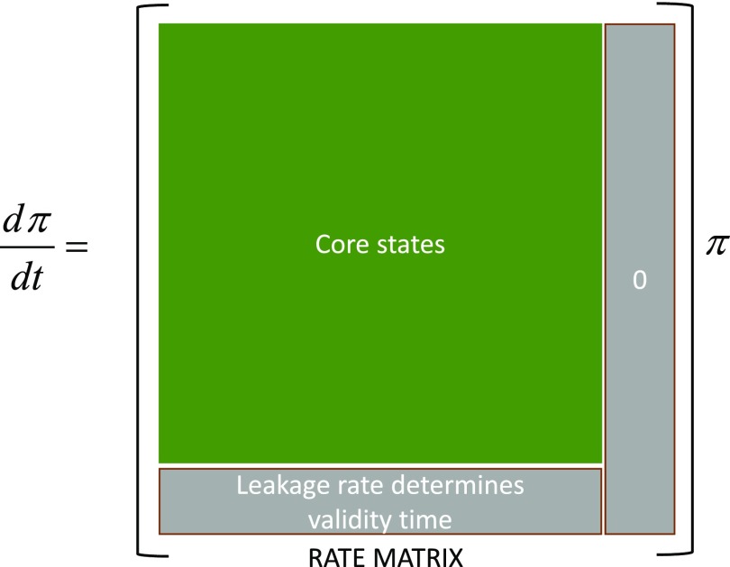
Figure 1 shows the structure of the rate matrix in Eq. (2) constructed with MD where core, periphery, and missing states are considered. Each off-diagonal term in the row (column) j in the matrix denotes the kinetic rates into (from) the state j. Core (periphery and missing) states are placed at the top (bottom) of the occupation vector on the right-hand side of Eq. (2). The matrix can be divided into three parts. The top-left (green) corner involves the core states, i.e., it forms the rate matrix for the MSM. We lump the periphery and missing states together as absorbing states. The last column of the matrix contains the rates from the absorbing states. The rates are set to zero. The bottom row of the matrix contains estimates of rates (termed leakage rates) from the core states to the absorbing states. As we shall show next, the validity time of the MSM is determined by the leakage rates, which in turn depends on the time spent in the core states. The validity time for the core network can be made large when all leakage rates are kept small.
FIG. 1.
Structure of a rate matrix in the master equation [Eq. (2)] when independent MD trajectories are used to build a Markov state model (MSM). denotes the occupation column vector.
B. Upper bound for the missing rate from a core state
Consider a collection of pathways from a state S with total rate k. Assuming first order kinetics, the probability of not selecting these paths in time spent in S is . The likelihood that the rate equals given that these paths are not selected in MD is . All values of k that result in likelihood greater than satisfy . Thus, can be regarded as a confidence associated with the estimate for k. An upper bound for the missing rates for a core state S is given by
| (3) |
Note that the entire MD duration . Similarly, an upper bound for the missing flux consistent with the MD data is .
C. Leakage flux from core network
For a core state S, Eq. (1) can be rewritten in terms of the core (C), periphery (P), and missing (M) states as
| (4) |
where the leakage flux
| (5) |
In the worst-case scenario, using Eq. (3) to replace FS with an upper bound, we define the maximum leakage flux from S as
| (6) |
The caret denotes maximum leakage into the periphery/missing states. State occupations are obtained by solving
| (7) |
The leakage flux can be ignored when . Once a state with large leakage is detected, one can analyze the source of leakage. Large leakage due to implies additional MD in state S would be beneficial. The other possibility is that one or more periphery states have become important to the dynamics. By performing additional MD, a periphery state is converted into a core state and its contribution to the leakage flux is eliminated. The flux from the core to periphery states is determined by the network topology. Topologies where the core states are connected to a large number of periphery states generally have a short validity time. The missing flux from state S can be made small by performing MD calculations in S, which extends the time tS.
The occupation is obtained by solving the MSM,
| (8) |
Detailed balance is not assumed, i.e., presence of both forward and backward pathways is not required. Dynamics from the core network [Eq. (8)] and full network [Eq. (7)] models diverge beyond the validity time. Consider a special case where the stationary distribution is attained and leakage in the full network model becomes significant at time scale beyond the relaxation time scales. We write
| (9) |
Since the core network dynamics is fast, the ratio of occupations for two core states is fixed, i.e., with denoting the probability of residing in the core states at time . Equation (9) is rewritten as
| (10) |
and
| (11) |
Here, denotes the total leakage rate for the network. The occupation for a core state S is
| (12) |
In general, Eqs. (7) and (8) need to be solved simultaneously to determine the validity time for the core network. For convenience, we can approximate the validity time scale in terms of the time constant for leakage, namely,
| (13) |
According to Eq. (12), the core state occupations decrease by a factor of exp(−1) at these time scales. The advantage of Eq. (13) is that only the core network model needs to be solved to calculate the validity time using Eq. (11). The assumption in Eqs. (11)–(13) that the relaxation time scale within the core network is smaller than the time scale associated with probability leakage is violated when the MD time accumulated in core state(s) is shorter than the relaxation time scale. We shall consider this case in Sec. III B. Note that in this work, a version of Eq. (13) using the time-dependent occupations is employed for calculating the validity time.
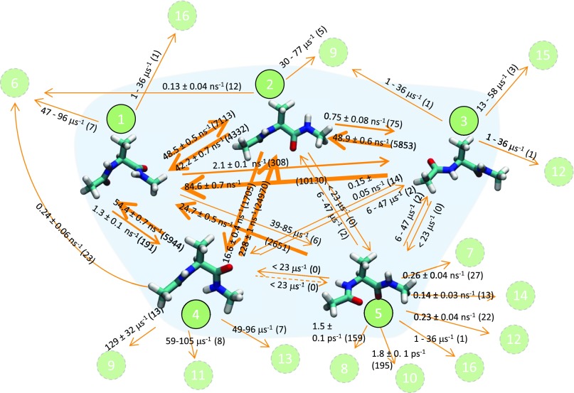
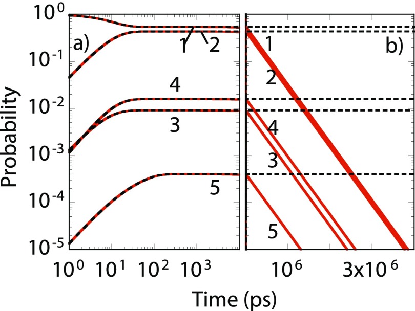
As an illustration, a MSM constructed for solvated alanine dipeptide at 300 K is shown in Fig. 2. States and kinetic pathways were found by analyzing on-the-fly several thousand MD trajectories as they were being generated in parallel. See Sec. S3 of the supplementary material for details regarding setup and comparison to literature results. States 1-5 form the core network. Detection of states 1-4 is possible within 0.1 μs MD, while detection of state 5 can require longer trajectories. States 1 and 3 closely represent the conformation of alanine dipeptide. States 2 and 4 are located in the β/PII/C7eq region in space. Occasionally, the system will visit 11 other states (see Fig. 2) only to quickly return to the core states. We consider these 11 states as periphery states. Kinetic rates were estimated using MLE when a pathway is sighted 10 times or more. Standard error in rates shown in Fig. 2 is computed using the Bootstrap method. Figure 3 shows the core state occupation in dashed lines obtained by solving Eq. (8). Although the MD trajectory exceeds 0.3 μs, it is conceivable that in the worst-case scenario absorbing-states will be visited via pathways that are missing in the core network model. The leakage flux, calculated based on the rates from core states to periphery states and the missing rate from each core state using , is included in the full network model of Eq. (7). Equations (7) and (8) agree at short times [Fig. 3(a)]; however, they diverge at longer time scales [Fig. 3(b)]. In the worst case, all core state occupations will decay exponentially with the same rate consistent with Eq. (9).
FIG. 2.
Markov state model for solvated alanine dipeptide at 300 K. States are numbered in the order they were discovered with MD. States 1-5 are core states and 6-16 are periphery states. Kinetic rates are shown along with the number of sightings for the event in parentheses.
FIG. 3.
Occupation for core states (states 1-5) of Fig. 2 found by solving the core network [Eq. (8), dashed black line] and full network [Eq. (7), red line] models at (a) short (log-log) and (b) long (semilog) time scales. Both models were constructed using MD trajectories. The full network model denotes the worst-case scenario where probability leakage into periphery/missing states occurs because of which the core state occupations decay exponentially at long time scales. The core network model is a compact MSM that does not contain any periphery/missing states.
Suppose the system is trapped/equilibrated in N core states corresponding to deep basins in the energy landscape and periphery states are absent, the MD time for a core state S is proportional to , i.e., . Equation (11) simplifies to
| (14) |
Subsequent coarse-graining of states into superstates can result in a more compact MSM, but the validity time is still determined by the total time spent in the superstate.
D. Programmed state constrained MD
Adaptive sampling methods50,57 that seek rare-configurations so that new MD trajectories can be seeded from such configurations are generally used for calculating thermodynamic properties. Relevant kinetic information can be gained by efficiently extending the MSM validity time. If state S is poorly sampled in a dynamical trajectory even though it is relevant, one will require a longer trajectory with the hope that at some point enough transitions from the state will be sampled. Such situations can be tackled using state-constrained MD calculations. In state-constrained MD calculations, one performs MD in state S while checking for a transition at regular intervals. Once a transition is detected, the MD calculation is stopped and the waiting time and final state are noted. A fresh independent MD calculation is seeded from S such that the system is in thermal equilibrium (see Sec. S1 of the supplementary material for flowchart). More transitions from S are sought. This prevents the system from freely diffusing over the potential energy landscape and confines it to a particular state for the purpose of detecting kinetic pathways from the state, calculating the rates, and lowering leakage flux of state S. Core- and full-network models can be constructed efficiently with programmed state-constrained MD (PSC-MD) by automatically targeting states with the largest leakage flux and performing state-constrained MD in those states (see Sec. S2 of the supplementary material for flowchart).
The PSC-MD scheme usually introduces many periphery states in the network model as it is used to build the MSM in patches. Occasionally, states are chosen from one part of the network for state-constrained MD calculations, and later, another part may be selected based on the calculated leakage flux. When the largest leakage is from core state S to a periphery state , state-constrained MD is performed in until becomes a core state. To achieve this goal with regular MD, a trajectory of duration is required, where m denotes the number of transitions needed for estimating the rate with reasonable statistical accuracy and kf is the fastest rate from . When the occupation is small, the time taken using state-constrained MD calculations given by is orders of magnitude smaller than the one using regular MD.
III. PROTOTYPE EXAMPLES
That the validity time is a vital parameter for quantifying the MSM accuracy becomes evident by examining simple networks that are fully known to us from the outset. We consider (i) a landscape containing trapping states, which is representative of deep basins of protein systems, and (ii) random walk in a corrugated landscape containing shallow basins reminiscent of a disordered system. This understanding will be useful later when we study stretched deca-alanine in Sec. IV.
A. Network with trapping states
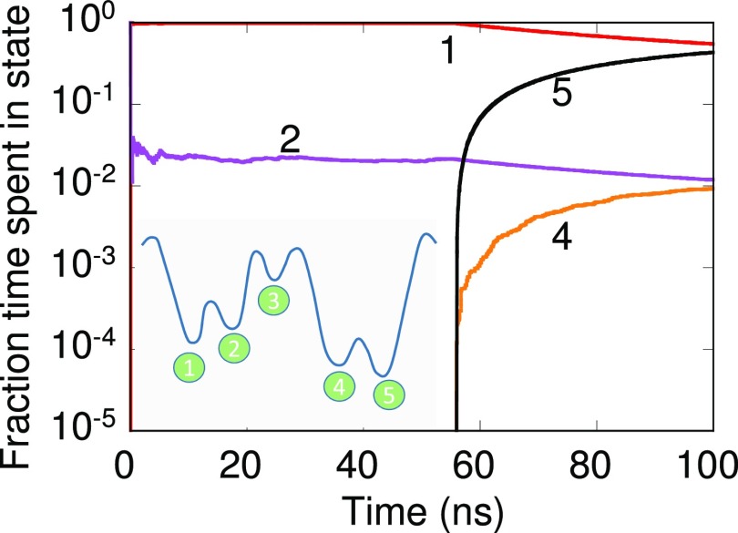
Energy landscapes of biomolecular systems often contain low lying minima separated by large barriers. The inset of Fig. 4 shows a one-dimensional network with 5 states. Initially the system is in state 2. The rate is calculated as , where is the energy barrier given in the caption of Fig. 4, kB is the Boltzmann constant, and T = 300 K is the temperature. Since the barrier for the move from state 2 to 3 is large (0.35 eV), the system remains trapped in states 1-2 at short times. States 4 and 5, which are also kinetic traps, are accessed at longer times.
FIG. 4.
Fraction of time spent in states belonging to the 1-D network shown in the inset over the course of the simulation. The x-axis denotes the time elapsed in a dynamical trajectory. Energy barrier for forward moves from left to right are 0.3, 0.35, 0.1, and 0.2 eV. Barriers for backward moves from left to right are 0.2, 0.1, 0.45, and 0.3 eV. The system resides in state 2 at time t = 0 ps.
A dynamical trajectory is generated using a kinetic Monte Carlo procedure wherein a move is selected randomly from the current state with a probability proportional to its rate and the time is advanced by . Here, is a uniform random deviate and kS is the sum of rates from the current state S. A MSM is constructed with the help of the dynamical trajectory. Kinetic rates are estimated using MLE when a pathway is sighted 10 times or more.
The fraction of time spent in a state in the dynamical trajectory is plotted in Fig. 4. After the initial transient, the occupations for states 1-2 plateau. Based on the short dynamical trajectory, one may correctly conclude that the MSM containing only states 1-2 will suffice at short time scales. The picture changes at the longer time scales. After 50 ns states 4-5 are accessed and the fraction of time spent in states 1-2 decays. State 3 is not shown in Fig. 4 for convenience. Similar behavior is expected from other dynamical trajectories started from state 2, although the time required to access states 4-5 will vary. The relevance of state 3 cannot be ignored as it provides access to states 4-5. Thus, the MSM should include states 1-5 at longer time scales. So when should one include states 3-5 to ensure that the MSM remains accurate?
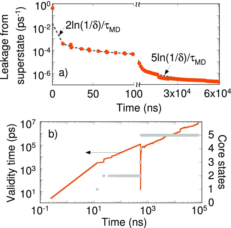
PSC calculations were performed with state 2 as the starting state. The validity time is calculated using . Initially, the MSM contains only two states and the MSM validity is extended by performing state-constrained calculations in states 1-2. The leakage rate from Eq. (14), namely, , is in close agreement with PSC calculations [Fig. 5(a)]. The validity time keeps increasing with the MD time except for an abrupt decrease when the periphery states 3-5 are detected [Fig. 5(b)]. All states and pathways were available in the MSM at 553 ns. The corresponding validity time was 20.1 ns. Although we are aware of the total number of states and pathways in this toy model, in general for complex systems such as proteins whether the network model is complete will remain unknown to us. Therefore, one would continue to search for newer states and pathways. At longer times, the leakage rate is given by .
FIG. 5.
(a) Leakage flux calculated using Eq. (14) (dashed line) and state-constrained calculations (filled circles). (b) Validity time calculated for the MSM constructed for the network in Fig. 4 using state-constrained calculations (orange line). The number of core states shown in filled grey circles increases as the trajectory grows longer. The x-axis in both panels denotes time elapsed in the dynamical trajectory.
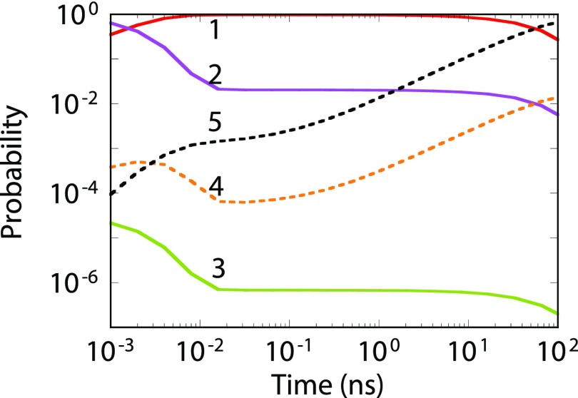
It can be shown that the fraction of time spent in states 1-2 is identical for the dynamical trajectory of Fig. 4 and the state-constrained calculations of Fig. 5 at short times. Similar behavior is true for states 4-5 at longer times. Therefore, conclusions from Fig. 5(b) can be extended to Fig. 4. From Fig. 5(b), a MSM generated from a 40 ns long dynamical trajectory is valid only till 8 ns. The MSM of Fig. 4 only contains the pathways between states 1-2 at 40 ns, i.e., the pathways missing in the MSM are less relevant to the dynamics till approximately 8 ns. This is confirmed in Fig. 6, where the time-dependent state occupations are plotted. States 3-5 are visited before 60 ns in Fig. 4, which corresponds to a validity time of approximately 10 ns. This implies states 1-5 should be present in a MSM when 10 ns time scales are accessed. Figure 6 shows that roughly in 1 in 10 dynamical trajectories the system will be in state 5 at 10 ns. When 1/10 is set as the tolerance limit, the dynamical behavior can no longer be predicted using a two-state MSM, highlighting the importance of missing pathways.
FIG. 6.
State occupation for the network shown in Fig. 3 obtained by solving the MSM with validity time of 104 ns. Initial state is 2.
B. Network with diffusive behavior
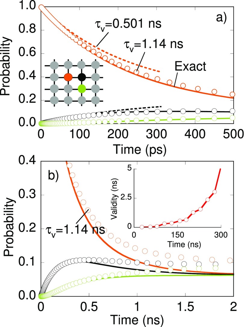
Dynamics in a large number of biomolecular and disordered systems can be described in terms of random walk in shallow energy basins. The inset of Fig. 7(a) shows a periodic 4 × 4 lattice where each site is connected to 4 neighboring sites, each pathway having a rate of 1 ns−1. A particle, initially placed at the orange-colored site, can randomly hop to any of its nearest-neighbor sites. The exact kinetic model contains 16 states and 64 pathways. The state occupation is obtained by solving the master equation analytically (solid lines in Fig. 7). Along the lines of Sec. III A, a MSM is constructed using PSC calculations of the total duration of 105 ns. Kinetic rates were estimated using MLE when a pathway is sighted 10 times or more. The MSM contains 4 core states, and the validity time calculated using Eq. (13) is 0.501 ns. Dashed lines in Fig. 7(a) denote the occupation obtained by solving this MSM. While the MSM predictions are reasonable at short time scales, deviations are observed later. The large leakage from core states to periphery states results in a small validity time in diffusing systems as shown in the inset of Fig. 7(b). A MSM constructed with 278 ns PSC calculations remains accurate for a longer period of time (see open-circles). The MSM contains 11 core states and has a validity time of 1.14 ns. All states and pathways are available in the core network model once PSC calculations have accrued 1045 ns.
FIG. 7.
State occupation calculated for MSMs of validity time 501 ps (dashed lines) and 1140 ps (open circles) at (a) short and (b) longer times. The MSM is constructed for the network in the inset of panel (a). Occupation for initial (orange), a nearest neighbor (black), and a next nearest neighbor (green) site is shown in their respective colors. Dependence of the validity time on the duration of the state constrained trajectory is shown in the inset of panel (b).
IV. MARKOV STATE MODEL OF STRETCHED DECA-ALANINE
Sections I–III lead to the conclusion that the MSM validity time is always shorter than the duration of MD used to construct the MSM. This has serious implications on long-time studies using MSMs. Despite this, crucial insights can be obtained with MSMs. We demonstrate this aspect by building a MSM with a desirable validity time to study the kinetics of a deca-alanine molecule in vacuum under tension. A capped deca-alanine (Ala10) with acetylated N-terminus and amidated C-terminus was selected for the study. The initial configuration was obtained from the 104-atom helical model of Ref. 58. The Cα atoms at the two ends (residues 1 and 10) are tethered to two anchor points by harmonic restraints with a spring constant of 0.86 (kcal/mol)/Å2 (Fig. 8 inset). The anchor separation d is kept fixed during the construction of a MSM and fluctuations in molecular extension, and forces are measured.
FIG. 8.
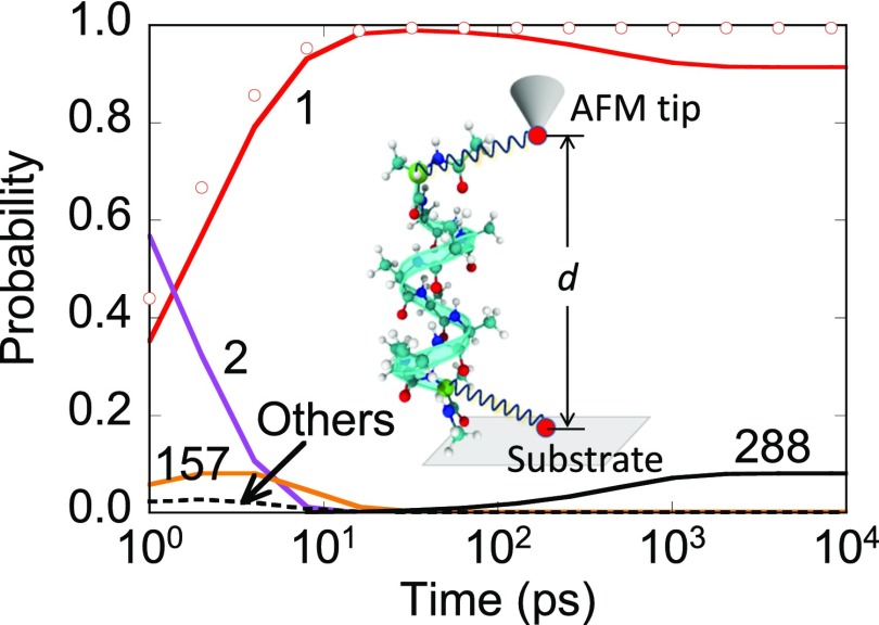
Occupation for the top-four states using a MSM with 65 ns validity time when the anchor separation d = 16 Å. The force-spectroscopy setup for deca-alanine in vacuum at 300 K is shown in the inset. Harmonic restraint is applied to the light-green colored Cα atoms. Open circles show state 1 occupation from a 5-state MSM with 2 ns validity time (constructed from a 0.57 μs long MD trajectory).
Past studies of deca-alanine demonstrate that unravelling of the helical structure results in higher free-energy configurations, although the presence of metastable configurations of stretched deca-alanine has not been reported. Hence, specific 3D metastable structures encountered in the dynamics are determined as d is varied between 16 and 26 Å. Questions related to appropriateness of employing the same Markov state definitions and pathways across different anchor separations as well as changes in the kinetic rates are examined. Analysis of dominant configurations helps us probe the importance of multiple pathways for unravelling of the helical structure as the molecule is stretched. Since helix winding/unwinding is a reversible process, helical and stretched configurations co-exist, which causes the force experienced by the AFM tip to fluctuate. Ensemble-average forces from MSMs and MD are compared. Through this study, we conclude that forces are inaccurately predicted using MSMs with short validity time, thus highlighting the important role of missing states/pathways in ensemble-averaged quantities.
MSMs are constructed on-the-fly with 90% confidence () using thousands of short-MD calculations that are run in parallel as part of the PSC procedure. All MD simulations were performed with NAMD 2.959 with the CHARMM36 force fields.60 Temperature was held at 300 K using a Langevin thermostat. Bonds involving hydrogen atoms were constrained to their equilibrium values using RATTLE.61 An integration time step of 2 fs was used. States were determined by comparing the backbone atoms after aligning the molecule using the Kabsch algorithm. A tolerance of 3 Å was found to be suitable for identifying the states. MD snapshots were collected every 0.2 ps because of rapid interconversion between the states. A transition was said to have successfully occurred when the system continues to reside in the new state for at least 1.2 ps after the transition was detected in the MD trajectory. This prevents recrossing events to be counted as transitions.
Steered MD simulations were performed with the deca-alanine for several nanoseconds to obtain a preliminary collection of unfolded structures. These configurations were provided as inputs to several nanosecond-long regular MD trajectories with chosen anchor separations. A preliminary catalog of states was constructed that could be employed with different anchor separations. States were indexed in the order they are found. State-constrained MD calculations, which are more efficient than regular MD (see Sec. II D), were used to confirm Markovian behavior (see Sec. S5 of the supplementary material) and that the kinetic pathways can be described as a first-order process. Poor MSM validity was achieved when states or MD duration were selected ad-hoc in the state-constrained MD calculations. For example, in a preliminary MSM-building attempt we found a 4 μs long MD trajectory resulted in a validity time of 0.064 ns, which is the reason why only PSC-MD calculations are performed.
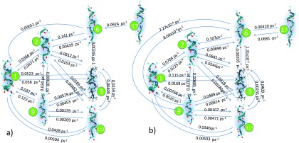
The full network model consisted of 810 states. Most states are periphery states. The number of core states and their relevance varies with anchor separation. State occupation at d = 16 Å obtained by solving a MSM of 65 ns validity is shown in Fig. 8. The MSM constructed using a 9 μs trajectory contains 25 core states and 78 pathways. The system was initially present in state 2 shown in Fig. 9. Rapid conversion to α-helical configuration (state 1) with a large rate of 0.44 ps−1 is observed consistent with previous studies. The average distance between the terminal Cα atoms is 16.4 Å for state 1. Another dominant configuration, namely state 288, is selected beyond 100 ps with nearly 10% probability. State 288 is accessible from state 1 with a small rate of 1.4 ns−1. As a consequence, state 288 is absent in a MSM with a shorter validity time and the time-dependent occupation for state 1 from such a MSM is incorrectly predicted (see open circles in Fig. 8). This behavior is analogous to the one observed in Fig. 4. State 288 is preferred over state 2 for two reasons. First, it has an end-to-end distance smaller than that of state 2, which is favored at compressive conditions. Second, the average α-helicity for states 1, 2, and 288 are 0.8, 0.2, and 0.74, respectively. Multiple backbone hydrogen bonds impart more stability to state 228 than state 2. It appears that a two-state model (states 1 and 288) might suffice for the calculation of average force at d = 16 Å.
FIG. 9.
Network model obtained when the anchor separation is (a) 22 and (b) 23 Å. Only frequently visited states are shown. State 3 (encircled) is the starting configuration for the subsequent figures.
The abundance of energetically-favorable stretched-out configurations causes state 288 to lose its relevance at higher anchor separations, but state 1 still continues to be relevant. Figure 9 shows the dominant core states for anchor separations 22 and 23 Å. The unravelling of a helical structure to an elongated one proceeds via multiple intermediate states. For instance, one pathway for visiting state 17 from state 1 involves only “local” readjustments. First, a partial opening of lower coils (C-terminal) is observed (state 1 to 6 via state 2) followed by subsequent stretching of the lower coils (state 6 to 17). Alternatively, fluctuations in the middle residues can frequently cause deformation in the helix (state 1 to 3) that may sometimes lead to an elongated configuration (state 3 to 6). States 2, 3, and 6 have a non-negligible 310-helicity (see Sec. S4B of the supplementary material). State 6, which is an essential intermediate for both pathways, can be reached faster from states 2 and 3 as the anchor separation is increased. The preferred winding/unwinding mechanism proceeds predominantly at the C-terminal, i.e., the former pathway.
In the past, the end-to-end distance has been employed as a reaction coordinate for stretched deca-alanine. End-to-end distance distribution for a state tends to be sharply-peaked with a standard deviation of nearly 1-2 Å; however, the distribution is a function of the anchor separation. Large overlap in end-to-end distribution for the core states makes it practically impossible to distinguish states when only end-to-end distances are employed. Inclusion of the 3D structure, which is implicit in our state description, helps resolve intermediate states and state-specific properties. In particular, we are interested in the stiffness of deca-alanine, which determines the force on the AFM tip. The stiffness, calculated using state-constrained MD calculations, is found to vary from one state to another depending on the intramolecular interactions. Presence of strong hydrogen bonds in state 1 results in a large spring constant of 39.44 pN/Å. On the other hand, state 3 has a smaller spring constant of 25.38 pN/Å. A natural consequence is that the average force experienced by the AFM tip can be altered by as much as 100 pN in either direction during a state-to-state transition because of the differences in the state-specific spring constants. The average force is given by the sum of force experienced for each state times the state occupations.
MSMs are sensitive to small changes in the anchor separation [see Figs. 9(a) and 9(b)]. Pathways between states 6 and 9 are absent in the MSM for d = 22 Å, but they are dynamically more relevant at validity times of 8 ns when d = 23 Å. Forward and backward rates are found for many pairs of states. Exceptions in Fig. 9(a) include the move from state 1 to 6, although this is not an issue since a stationary solution is obtained without the requirement of detailed balance. The rate constants involving the core states vary over several orders of magnitude between 10−1 and 10−5 ps−1. Exponential increase/decrease in rates is witnessed between 16 and 26 Å (see Sec. S4B of the supplementary material). While a handful states can describe the dynamics for small anchor separations, additional states should be included in the MSM when the molecule is stretched extensively. An explosion in the number of core states is witnessed from 36 to 78 states between 22 and 25 Å. Correspondingly, the validity time plummets by almost 10 times from 12 ns at 22 Å separation to 1.5 ns at 25 Å separation for a 0.5 μs long MD trajectory. Note the length of (PSC-)MD trajectory required to reach the nanosecond-long validity time.
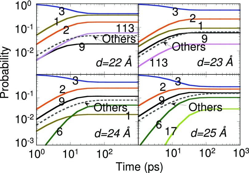
Figure 10 shows the evolution obtained with different MSMs for anchor separations between 22 and 25 Å. The rise and fall in the relevance of states and kinetic pathways is witnessed. The initial state of the system is state 3. One might expect that the helical structures (state 1) would not be selected at high separations; however, even at 24 Å separation there is a 1% chance of finding state 1. This is attributed to the lower energy of state 1 and the small stiffness of the tethers. In other words, it is possible for the tether to stretch to an extent where state 1 can still be visited in the dynamics at 24 Å separation. State 3 is an important configuration between 22 and 25 Å separation. The maximum state 3 occupation is witnessed around 23 Å. States 9, 6, and 17 compete with each other at large anchor separations. As the number of core states increases, there is an increased chance that the system will visit these states. The occupation in all other core states combined is shown in the dashed lines in Fig. 10. The time spent in the top-five states decreases from 96% at 22 Å separation to 30% at 26 Å separation. Based on Fig. 10, the stationary solution for deca-alanine is reached at nearly 100 ps, i.e., time-dependent forces can be resolved only at sub-100 ps time scales.
FIG. 10.
Probability evolution for different anchor separations. Numbers denote the state index in Fig. 9. The initial state of the system was state 3. The MSM validity time exceeded 1 ns in all cases.
The free energy difference for a state A with respect to state B is calculated from the stationary distribution as where p denotes the stationary occupation of a state. Since the stationary solution depends on the relevant pathways, absence of one or more pathways can introduce errors in the free energies. Occupations in Fig. 10 were used to calculate the free-energy difference between the states. Insights into the separation-dependence of the kinetic rates can be obtained from the Bell-Evans-Polyani principle.62,63 Consider states 1 and 2. Since the free energy of state 1 increases with reference to state 2 as deca-alanine is stretched, the free barrier for the move from 1 to 2 (2 to 1) decreases (increases), which explains the corresponding shift in the rate constants (see Sec. S4B of the supplementary material). Similarly, the free energy of state 2 decreases with respect to state 3, causing the rate constant from state 2 to 3 to increase. As shown in Sec. S4A of the supplementary material, the work done while stretching deca-alanine can be calculated using the stationary occupations at different anchor separations. The calculated work is in agreement with previous values in the literature.
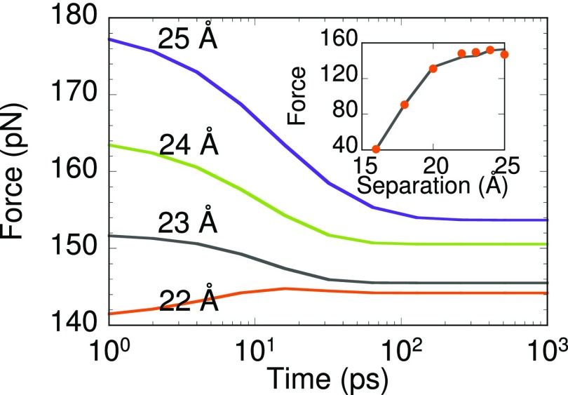
Figure 11 shows the time-dependent ensemble-averaged force experienced by the AFM tip corresponding to the evolution shown in Fig. 10 for different anchor separation. Average forces were computed for the individual core states using state-constrained MD. Since the force experienced with state 3 is smaller than with state 1, the average force increases with time at 22 Å separation as state 1 occupation increases (see Fig. 10). Although state 3 plays a minor role in the winding/unwinding of deca-alanine, it is important for calculation of average forces due to its large occupation. Beyond 23 Å separation, one finds that state 2 is preferred over state 3. The average force decreases with time since the force experienced with state 2 is smaller than with state 3. The average force at steady-state from the MSM and MD are in good agreement (Fig. 11 inset) validating our MSM. Such an agreement between MD and the MSM is not witnessed when the validity time is small as many relevant states are missing. The sudden drop in the slope of the force-separation curve is attributed to the smaller stiffness of states encountered at higher separations.
FIG. 11.
Solid lines show the average force acting on the AFM tip when the deca-alanine is stretched (using MSMs with validity time exceeding 4 ns). Behavior for anchor separation 22-25 Å is shown. Steady state forces calculated from the MSM (line) and MD (filled-circles) shown in inset are in good agreement.
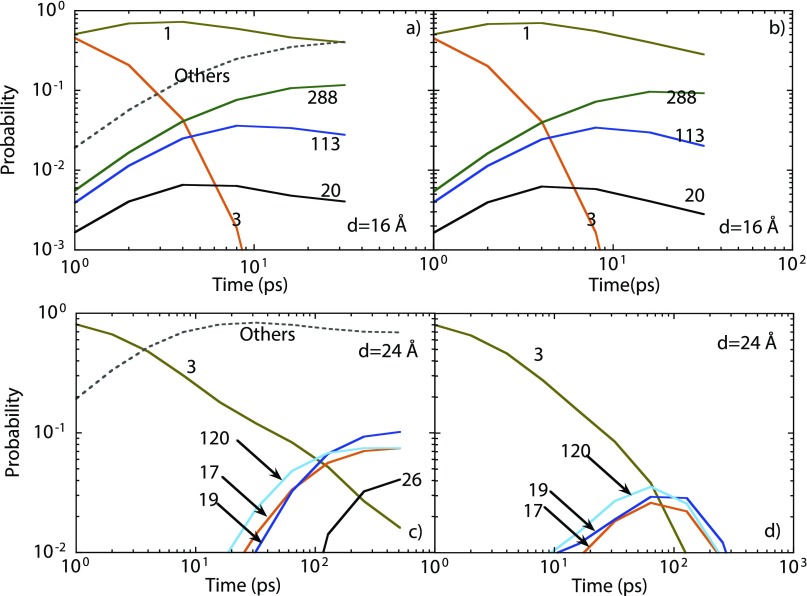
Weaker electrostatic interactions are expected when deca-alanine is present in water. To mimic the effect of water, we construct MSMs at anchor separations 16 and 24 Å with a dielectric constant of 80. In order to find common features in the dynamical behavior for dielectric constants 1 and 80, the list of 810 states obtained previously was used as the starting known structures for our new calculations. Deca-alanine was initially kept in state 3. The dominant states for anchor separation of 16 Å include states 1, 20, 113, and 288. Figure 12(a) shows that the occupation for state 3 decreases continually in time. As in Fig. 8, a maximum value of the occupation for state 1 is witnessed. However, the steady state occupation for state 1, namely, 0.401, is much smaller than the one observed in Fig. 8. The occupation for other states combined increases to a significant value. We find that 11 states possess steady state occupations greater than 0.01. By considering the full network model, we conclude that the MSM obtained with 10.8 ns long MD calculations has a validity time of nearly 30 ps. At 30 ps, the difference in the state 1 occupations in the MSM and the full network model has exceeded 0.1. More states are observed with the anchor separation of 24 Å. In all 25 states possessed a steady state occupation in excess of 0.01 with state 3 being the only state common to both Figs. 10 and 12 with d = 24 Å. The total number of core states was found to be 137 using 53 ns long PSC-MD. Figures 12(c) and 12(d) show state occupations as a function of time from the MSM and the full network model. Predictions from the two models diverge at nearly 0.1 ns. One can determine whether states and kinetic pathways in the present MSM will continue to remain relevant at longer time scales only by extending the validity time of the MSM.
FIG. 12.
Probability evolution for anchor separations 16 Å [panels (a) and (b)] and 24 Å [panels (c) and (d)] using the dielectric constant of 80 to mimic deca-alanine in water. Numbers denote state index. Initial state of the system was state 3. Left panels [(a) and (c)] show results from the MSM while right panels [(b) and (d)] show results obtained with the full network model.
V. CONCLUSIONS
MSMs have the potential to become even more powerful computational tools in the future for studies of biomolecular, materials, and reacting systems as new advances emerge that enable one to accurately encode the kinetic and thermodynamic information on the multidimensional landscape in terms of state-to-state transitions. Unfortunately, MSMs constructed bottom-up from finite MD trajectories are rarely complete, which has a direct implication on its accuracy. Since the (kinetic) information content in a single trajectory can be different from that of an ensemble at the same length of time, questions related to validity of the MSM due to missing information arise. We introduce the fundamental concept of validity time of a MSM to quantify its completeness. The concept guarantees that all states and kinetic pathways that are relevant to the dynamics will be present in the MSM provided the time scales accessed by the model are smaller than its validity time. Put differently, this concept helps us understand the time scales where states and pathways missing in the available MD data or the MSM can become relevant to experimentally measurable quantities, and differences between the experimental quantities and MSM predictions might originate from the missing information in the MSM. Our methodology is flexible in terms of its ability to handle a wide-range of kinetic rates, number of states, relaxation times in the network, topology of the network, as well as missing pathways and states that have not been found with MD. Development of programmed state-constrained MD calculations in this work provides an efficient means for extending validity time of a MSM.
MSMs with sufficiently large validity time provide following key insights into the stretching of deca-alanine. Unwinding of deca-alanine proceeds mainly via breaking of hydrogen bonds at the C-terminal. Characterization of states might not be possible only using simple reaction coordinates such as end-to-end distance. Each state possesses its own mechanical characteristics, e.g., spring constants, that ultimately determine the force experienced by the AFM tip in the force spectroscopy (FS) setup. To calculate the force, one also needs to accurately estimate the state occupations. It is not straightforward to guess the relevant states/pathways at different anchor separations. The list of relevant states and kinetic pathways, and associated rates, i.e., the network topology, can change dramatically with the anchor separation. The size of the MSM increases for large anchor separations, which has a direct bearing on the amount of MD required to know the state occupations accurately. Our studies demonstrate that the absence of relevant states/pathways in the MSM can lead to incorrect prediction of the kinetic and thermodynamic quantities being sought, which is the main reason why studies employing MSMs and other related kinetic network models should state the validity time of the model.
SUPPLEMENTARY MATERIAL
See supplementary material for the flow chart for state constrained and programmed state constrained MD, simulation protocol used for solvated alanine dipeptide, additional figures for the deca-alanine system, and discussion on test for Markovian behavior.
ACKNOWLEDGMENTS
A.C. acknowledges support from Science and Engineering Research Board, Department of Science and Technology Grant No. SB/S3/CE/022/2014 and Indian National Science Academy Grant No. SP/YSP/120/2015/307. S.B. acknowledges support from Department of Biotechnology Grant No. BT/PR8311/BID/7/451/2013.
REFERENCES
- 1.Schwantes C. R., McGibbon R. T., and Pande V. S., J. Chem. Phys. 141, 090901 (2014). 10.1063/1.4895044 [DOI] [PMC free article] [PubMed] [Google Scholar]
- 2.Pande V. S., Beauchamp K., and Bowman G. R., Methods 52, 99 (2010). 10.1016/j.ymeth.2010.06.002 [DOI] [PMC free article] [PubMed] [Google Scholar]
- 3.Senne M., Trendelkamp-Schroer B., Mey A. S. J. S., Schütte C., and Noé F., J. Chem. Theory Comput. 8, 2223 (2012). 10.1021/ct300274u [DOI] [PubMed] [Google Scholar]
- 4.Buchete N.-V. and Hummer G., J. Phys. Chem. B 112, 6057 (2008). 10.1021/jp0761665 [DOI] [PubMed] [Google Scholar]
- 5.Schütte C., Noé F., Lu J., Sarich M., and Vanden-Eijnden E., J. Chem. Phys. 134, 204105 (2011). 10.1063/1.3590108 [DOI] [PubMed] [Google Scholar]
- 6.Gnanakaran S., Nymeyer H., and Portman J., Curr. Opin. Struct. Biol. 13, 168 (2003). 10.1016/s0959-440x(03)00040-x [DOI] [PubMed] [Google Scholar]
- 7.Dodson G. G., Lane D. P., and Verma C. S., EMBO Rep. 9, 144 (2008). 10.1038/sj.embor.7401160 [DOI] [PMC free article] [PubMed] [Google Scholar]
- 8.Klenin K., Strodel B., Wales D. J., and Wenzel W., Biochim. Biophys. Acta 1814, 977 (2011). 10.1016/j.bbapap.2010.09.006 [DOI] [PubMed] [Google Scholar]
- 9.Woodside M. T. and Block S. M., Annu. Rev. Biophys. 43, 19 (2014). 10.1146/annurev-biophys-051013-022754 [DOI] [PMC free article] [PubMed] [Google Scholar]
- 10.Chatterjee A. and Vlachos D. G., J. Comput.-Aided Mater. Des. 14, 253 (2007). 10.1007/s10820-006-9042-9 [DOI] [Google Scholar]
- 11.Voter A. F., in Radiation Effects in Solids, edited by Sickafus K. E., Kotomin E. A., and Uberuaga B. P. (Springer, NATO Publishing Unit, Dordrecht, 2006). [Google Scholar]
- 12.Wales D. J., Int. Rev. Phys. Chem. 25, 237 (2006). 10.1080/01442350600676921 [DOI] [Google Scholar]
- 13.Ziff R. M., Gulari E., and Barshad Y., Phys. Rev. Lett. 56, 2553 (1986). 10.1103/physrevlett.56.2553 [DOI] [PubMed] [Google Scholar]
- 14.Gilmer G. H., Huang H. C., de la Rubia T. D., Dalla Torre J., and Baumann F., Thin Solid Films 365, 189 (2000). 10.1016/s0040-6090(99)01057-3 [DOI] [Google Scholar]
- 15.Haldar P. and Chatterjee A., Acta Mater. 127, 379 (2017). 10.1016/j.actamat.2017.01.049 [DOI] [Google Scholar]
- 16.Chatterjee A., Katsoulakis M. A., and Vlachos D. G., Phys. Rev. E 71, 026702 (2005). 10.1103/physreve.71.026702 [DOI] [PubMed] [Google Scholar]
- 17.Chatterjee A. and Voter A. F., J. Chem. Phys. 132, 194101 (2010). 10.1063/1.3409606 [DOI] [PubMed] [Google Scholar]
- 18.Chatterjee A. and Vlachos D. G., J. Chem. Phys. 124, 64110 (2006). 10.1063/1.2166380 [DOI] [PubMed] [Google Scholar]
- 19.Weinan E., Engquist B., and Huang Z. Y., Phys. Rev. B 67, 092101 (2003). 10.1103/physrevb.67.092101 [DOI] [Google Scholar]
- 20.Snyder M. A., Chatterjee A., and Vlachos D. G., Comput. Chem. Eng. 29, 701 (2004). 10.1016/j.compchemeng.2004.09.016 [DOI] [Google Scholar]
- 21.Bowman G. R., Huang X., and Pande V. S., Methods 49, 197 (2009). 10.1016/j.ymeth.2009.04.013 [DOI] [PMC free article] [PubMed] [Google Scholar]
- 22.Chodera J. D., Singhal N., Pande V. S., Dill K. A., and Swope W. C., J. Chem. Phys. 126, 155101 (2007). 10.1063/1.2714538 [DOI] [PubMed] [Google Scholar]
- 23.Prinz J.-H., Wu H., Sarich M., Keller B., Senne M., Held M., Chodera J. D., Schütte C., and Noé F., J. Chem. Phys. 134, 174105 (2011). 10.1063/1.3565032 [DOI] [PubMed] [Google Scholar]
- 24.Xu L. and Henkelman G., J. Chem. Phys. 129, 114104 (2008). 10.1063/1.2976010 [DOI] [PubMed] [Google Scholar]
- 25.Konwar D., Bhute V. J., and Chatterjee A., J. Chem. Phys. 135, 174103 (2011). 10.1063/1.3657834 [DOI] [PubMed] [Google Scholar]
- 26.Voter A. F., J. Chem. Phys. 106, 4665 (1997). 10.1063/1.473503 [DOI] [Google Scholar]
- 27.Laio A. and Parrinello M., Proc. Natl. Acad. Sci. U. S. A. 99, 12562 (2002). 10.1073/pnas.202427399 [DOI] [PMC free article] [PubMed] [Google Scholar]
- 28.Ensing B., De Vivo M., Liu Z., Moore P., and Klein M. L., Acc. Chem. Res. 39, 73 (2006). 10.1021/ar040198i [DOI] [PubMed] [Google Scholar]
- 29.Voter A. F., Montalenti F., and Germann T. C., Annu. Rev. Mater. Res. 32, 321 (2002). 10.1146/annurev.matsci.32.112601.141541 [DOI] [Google Scholar]
- 30.Divi S. and Chatterjee A., J. Chem. Phys. 140, 184115 (2014). 10.1063/1.4875476 [DOI] [PubMed] [Google Scholar]
- 31.Imandi V. and Chatterjee A., J. Chem. Phys. 145, 034104 (2016). 10.1063/1.4958834 [DOI] [PubMed] [Google Scholar]
- 32.Haldar P. and Chatterjee A., Modell. Simul. Mater. Sci. Eng. 23, 025002 (2015). 10.1088/0965-0393/23/2/025002 [DOI] [Google Scholar]
- 33.Bhute V. J. and Chatterjee A., J. Chem. Phys. 138, 244112 (2013). 10.1063/1.4812319 [DOI] [PubMed] [Google Scholar]
- 34.Bhute V. J. and Chatterjee A., J. Chem. Phys. 138, 084103 (2013). 10.1063/1.4792439 [DOI] [PubMed] [Google Scholar]
- 35.Chill S. T. and Henkelman G., J. Chem. Phys. 140, 214110 (2014). 10.1063/1.4880721 [DOI] [PubMed] [Google Scholar]
- 36.Chatterjee A. and Bhattacharya S., J. Chem. Phys. 143, 114109 (2015). 10.1063/1.4930976 [DOI] [PubMed] [Google Scholar]
- 37.Chatterjee A. and Bhattacharya S., J. Phys.: Conf. Ser. 759, 012024 (2016). 10.1088/1742-6596/759/1/012024 [DOI] [Google Scholar]
- 38.Mu Y., Nguyen P. H., and Stock G., Proteins 58, 45 (2005). 10.1002/prot.20310 [DOI] [PubMed] [Google Scholar]
- 39.Kellogg E. H., Lange O. F., and Baker D., J. Phys. Chem. B 116, 11405 (2012). 10.1021/jp3044303 [DOI] [PubMed] [Google Scholar]
- 40.Zhou T. and Caflisch A., J. Chem. Theory Comput. 8, 2930 (2012). 10.1021/ct3003145 [DOI] [PubMed] [Google Scholar]
- 41.McGibbon R. T. and Pande V. S., J. Chem. Theory Comput. 9, 2900 (2013). 10.1021/ct400132h [DOI] [PubMed] [Google Scholar]
- 42.Pérez-Hernández G., Paul F., Giorgino T., de Fabritiis G., and Noé F., J. Chem. Phys. 139, 015102 (2013). 10.1063/1.4811489 [DOI] [PubMed] [Google Scholar]
- 43.Schwantes C. R. and Pande V. S., J. Chem. Theory Comput. 9, 2000 (2013). 10.1021/ct300878a [DOI] [PMC free article] [PubMed] [Google Scholar]
- 44.Beauchamp K. A., Bowman G. R., Lane T. J., Maibaum L., Haque I. S., and Pande V. S., J. Chem. Theory Comput. 7, 3412 (2011). 10.1021/ct200463m [DOI] [PMC free article] [PubMed] [Google Scholar]
- 45.Ghosh S., Chatterjee A., and Bhattacharya S., J. Chem. Theory Comput. 13, 957–962 (2017). 10.1021/acs.jctc.6b01094 [DOI] [PubMed] [Google Scholar]
- 46.Ensign D. L. and Pande V. S., J. Phys. Chem. B 113, 12410 (2009). 10.1021/jp903107c [DOI] [PubMed] [Google Scholar]
- 47.Sarich M., Noé F., and Schütte C., Multiscale Model. Simul. 8, 1154 (2010). 10.1137/090764049 [DOI] [Google Scholar]
- 48.Djurdjevac N., Sarich M., and Schütte C., Multiscale Model. Simul. 10, 61 (2012). 10.1137/100798910 [DOI] [Google Scholar]
- 49.Metzner P., Noé F., and Schütte C., Phys. Rev. E 80, 021106 (2009). 10.1103/physreve.80.021106 [DOI] [PubMed] [Google Scholar]
- 50.Bowman G. R., J. Chem. Phys. 137, 134111 (2012). 10.1063/1.4755751 [DOI] [PMC free article] [PubMed] [Google Scholar]
- 51.Zhou T. and Caflisch A., J. Chem. Theory Comput. 8, 2134 (2012). 10.1021/ct300147t [DOI] [PubMed] [Google Scholar]
- 52.Faradjian A. K. and Elber R., J. Chem. Phys. 120, 10880 (2004). 10.1063/1.1738640 [DOI] [PubMed] [Google Scholar]
- 53.Maragliano L. and Vanden-Eijnden E., Chem. Phys. Lett. 426, 168 (2006). 10.1016/j.cplett.2006.05.062 [DOI] [Google Scholar]
- 54.Laio A. and Gervasio F., Rep. Prog. Phys. 71, 126601 (2008). 10.1088/0034-4885/71/12/126601 [DOI] [Google Scholar]
- 55.Pan A. C., Sezer D., and Roux B., J. Phys. Chem. B 112, 3432 (2008). 10.1021/jp0777059 [DOI] [PMC free article] [PubMed] [Google Scholar]
- 56.de Oliveira C. A. F., Hamelberg D., and McCammon J. A., J. Chem. Phys. 127, 175105 (2007). 10.1063/1.2794763 [DOI] [PubMed] [Google Scholar]
- 57.Huang X., Bowman G. R., Bacallado S., and Pande V. S., Proc. Natl. Acad. Sci. U. S. A. 106, 19765 (2009). 10.1073/pnas.0909088106 [DOI] [PMC free article] [PubMed] [Google Scholar]
- 58.Park S., Khalili-Araghi F., Tajkhorshid E., and Schulten K., J. Chem. Phys. 119, 3559 (2003). 10.1063/1.1590311 [DOI] [Google Scholar]
- 59.Phillips J. C., Braun R., Wang W., Gumbart J., Tajkhorshid E., Villa E., Chipot C., Skeel R. D., Kalé L., and Schulten K., J. Comput. Chem. 26, 1781 (2005). 10.1002/jcc.20289 [DOI] [PMC free article] [PubMed] [Google Scholar]
- 60.Best R. B., Zhu X., Shim J., Lopes P. E. M., Mittal J., Feig M., and Mackerell A. D., J. Chem. Theory Comput. 8, 3257 (2012). 10.1021/ct300400x [DOI] [PMC free article] [PubMed] [Google Scholar]
- 61.Andersen H. C., J. Comput. Phys. 52, 24 (1983). 10.1016/0021-9991(83)90014-1 [DOI] [Google Scholar]
- 62.Evans M. G. and Polanyi M., Trans. Faraday Soc. 31, 875 (1935). 10.1039/tf9353100875 [DOI] [Google Scholar]
- 63.Marcus R. A., J. Phys. Chem. 72, 891 (1968). 10.1021/j100849a019 [DOI] [Google Scholar]
Associated Data
This section collects any data citations, data availability statements, or supplementary materials included in this article.
Supplementary Materials
See supplementary material for the flow chart for state constrained and programmed state constrained MD, simulation protocol used for solvated alanine dipeptide, additional figures for the deca-alanine system, and discussion on test for Markovian behavior.


