

Abstract
Purpose
Many radiomics features were originally developed for non‐medical imaging applications and therefore original assumptions may need to be reexamined. In this study, we investigated the impact of slice thickness and pixel spacing (or pixel size) on radiomics features extracted from Computed Tomography (CT) phantom images acquired with different scanners as well as different acquisition and reconstruction parameters. The dependence of CT texture features on gray‐level discretization was also evaluated.
Methods and materials
A texture phantom composed of 10 different cartridges of different materials was scanned on eight different CT scanners from three different manufacturers. The images were reconstructed for various slice thicknesses. For each slice thickness, the reconstruction Field Of View (FOV) was varied to render pixel sizes ranging from 0.39 to 0.98 mm. A fixed spherical region of interest (ROI) was contoured on the images of the shredded rubber cartridge and the 3D printed, 20% fill, acrylonitrile butadiene styrene plastic cartridge (ABS20) for all phantom imaging sets. Radiomic features were extracted from the ROIs using an in‐house program. Features categories were: shape (10), intensity (16), GLCM (24), GLZSM (11), GLRLM (11), and NGTDM (5), fractal dimensions (8) and first‐order wavelets (128), for a total of 213 features. Voxel‐size resampling was performed to investigate the usefulness of extracting features using a suitably chosen voxel size. Acquired phantom image sets were resampled to a voxel size of 1 × 1 × 2 mm3 using linear interpolation. Image features were therefore extracted from resampled and original datasets and the absolute value of the percent coefficient of variation (%COV) for each feature was calculated. Based on the %COV values, features were classified in 3 groups: (1) features with large variations before and after resampling (%COV >50); (2) features with diminished variation (%COV <30) after resampling; and (3) features that had originally moderate variation (%COV <50%) and were negligibly affected by resampling. Group 2 features were further studied by modifying feature definitions to include voxel size. Original and voxel‐size normalized features were used for interscanner comparisons. A subsequent analysis investigated feature dependency on gray‐level discretization by extracting 51 texture features from ROIs from each of the 10 different phantom cartridges using 16, 32, 64, 128, and 256 gray levels.
Results
Out of the 213 features extracted, 150 were reproducible across voxel sizes, 42 improved significantly (%COV <30, Group 2) after resampling, and 21 had large variations before and after resampling (Group 1). Ten features improved significantly after definition modification effectively removed their voxel‐size dependency. Interscanner comparison indicated that feature variability among scanners nearly vanished for 8 of these 10 features. Furthermore, 17 out of 51 texture features were found to be dependent on the number of gray levels. These features were redefined to include the number of gray levels which greatly reduced this dependency.
Conclusion
Voxel‐size resampling is an appropriate pre‐processing step for image datasets acquired with variable voxel sizes to obtain more reproducible CT features. We found that some of the radiomics features were voxel size and gray‐level discretization‐dependent. The introduction of normalizing factors in their definitions greatly reduced or removed these dependencies.
Keywords: computed tomography, features, gray levels, phantom, radiomics, texture, voxel size
1. Introduction
The techniques of extracting useful quantitative information from medical images, known as radiomics, holds promise for early detection, risk assessment, and treatment decisions in oncology.1, 2, 3 During the last decade, studies have highlighted the importance of texture analysis by connecting cancer imaging phenotypes captured by computed tomography (CT), and other imaging modalities, with underlying gene expression profiles in several cancer types.4, 5, 6, 7, 8, 9 Radiomics consists of several distinct processes including image acquisition and reconstruction, segmentation of the regions of interest, feature extraction and data analysis for subsequent model building. Every individual process in radiomics has its own problems and challenges.10 The challenges relevant to robustness of radiomic features because of variations in image acquisition and reconstruction parameters in CT and other imaging modalities have been of recent interest.11, 12, 13 The standardization of certain CT parameters might be a prerequisite for the successful application of radiomics features as biomarkers for tumor phenotype, diagnosis, prognosis and/or decision support.14 One way to test the robustness of these features with varying acquisition and reconstruction parameters is to evaluate their fundamental characteristics using imaging phantoms such as the recently described texture phantom.15, 16 In other words, texture phantoms can be used to investigate the impact of CT parameters on radiomics features.
Pixel spacing (size) and slice thickness are two important CT parameters that vary significantly from protocol to protocol, across scanners and vendors, as well as per institutional preferences. In a recent study15, pixel spacing was varied from 0.49 to 0.98 mm and slice thickness from 2 to 3 mm across 17 different scanners. Resampling was performed to obtain in‐plane pixel spacing of 1 mm2 before feature calculation. A separate study of 74 lung cancer patients used 3 to 6 mm variation in slice thickness and a large variation in pixel spacing.17 A phantom study by Zhao et al., reported that slice thickness can largely impact radiomic features.18 The same authors recently reported that CT images reconstructed with different slice thickness and reconstruction kernels resulted in low reproducibility of most radiomic features.11 Given the variability of pixel spacing and slice thickness in standard of care imaging, it is important to study the impact of these parameters on radiomic features among multiple scanners and multiple vendors.
As radiomics strives to use standard of care images from different imaging modalities, an ideal method leading to automation would be to extract features from minimally or non‐curated images. In this respect, it would be necessary to arrive at a subset of robust radiomic features and minimal pre‐processing of images. In computed tomography, voxel size in a region of interest depends on both pixel dimensions (x‐y plane) and slice thickness (z‐axis), assuming slice thickness equals inter‐slice distance. Any change in these two parameters changes the CT image resolution or voxel size. A minimally curation step may be to resample image sets so that all have the same voxel size. In this paper, voxel‐size resampling was investigated as a way to minimize the variability in feature values because of differing voxel sizes.
Texture features extraction methodology is another important factor that has varied wildly from one research study to another. In particular, voxel intensities within a region of interest are typically resampled into a limited number of discrete values or bin sizes before calculating feature values.19 Different studies have used different gray‐level resampling before extracting texture features.8, 12, 20, 21, 22 Recently, the impact of SUV discretization on radiomics features in FDG‐PET indicated that there is a need for standardized methodology for conducting multi‐center studies.23 Therefore, it is important to determine how feature values behave as a function of the number of gray levels using stable texture phantoms with the intention of later applying rescaling or normalization factors that make features more reproducible.
The purpose of this study was to investigate the robustness of CT radiomic features from original and resampled datasets from multiple scanners and vendors and to identify features showing voxel size (volume) and/or number of voxels dependencies. Additionally, we evaluated CT texture features as a function of the number of gray levels. We identified features with intrinsic dependencies and in several cases were able to apply normalizing factors to improve robustness of these features.
2. Materials and methods
2.A. Acquisition and reconstruction
The phantom employed in this study was the Credence Cartridge Radiomics (CCR) phantom recently described by Mackin et al.15 Scans of the CCR Phantom were acquired using eight different CT scanners from three different manufactures: 2 General Electric (GE), 4 Siemens and 2 Philips Healthcare Systems (Table 1). One of the GE scanner employed was a PET/CT scanner (Discovery STE). Slice thicknesses for the Philips and Siemens scanners were 1.5, 2.0, and 3.0 mm and for the GE scanners were 1.25, 2.5, and 3.75 mm. The adjacent reconstruction interval or zero inter‐slice gap was used for all CT phantom scans. For every slice thickness, the reconstruction Field Of View (FOV) was varied from 200 to 500 mm, corresponding to pixel sizes ranging from 0.39 to 0.98 mm. Pixel size was calculated as FOV/matrix size and a matrix size of 512 by 512 was kept constant for all scans. The variation in voxel size was obtained by changing pixel size (5 FOVs per scanner) or slice thickness (3 slice thicknesses per scanner) for a total 8 CT scanners. Therefore, there was a total of 120 CT data sets for the voxel‐size resampling study. However, 4 CT datasets were corrupted during file transfer, therefore, 116 datasets were used for analysis. To facilitate interscanner comparison, similar acquisition and reconstruction parameters were used across different scanners as given in Table 1.
Table 1.
CT scanners and scanning parameters used in this study
| CT Scanner | KVp | mAs | Scan Type | Pitch | Rotation time (Sec) | Reconstruction Kernel | Detector Configuration (mm) |
|---|---|---|---|---|---|---|---|
| GE Discovery STE (GE1) | 120 | 250* | Helical | 0.984 | 1.0 | Standard | Det. Coverage = 40 |
| GE Lightspeed 32 pro (GE2) | 120 | 250* | Helical | 0.984 | 1.0 | Standard | Det. Coverage = 40 |
| Philips Big Bore (P1) | 120 | 250 | Helical | 1.024 | 1.0 | Standard (B) | 16 × 0.75 |
| Philips Brilliance 64 (P2) | 120 | 250 | Helical | 1.024 | 1.0 | Standard (B) | 64 × 0.625 |
| Siemens Definition AS (S1) | 120 | 250 | Helical | 1.0 | 1.0 | I31f‐2 | 64 × 0.625 |
| Siemens Sensation 64 (S2) | 120 | 250 | Helical | 1.0 | 1.0 | B31f | 64 × 0.625 |
| Siemens Sensation 40 (S3) | 120 | 250 | Helical | 1.0 | 1.0 | B31f | 40 × 0.625 |
| Siemens Sensation 16 (S4) | 120 | 250 | Helical | 1.0 | 1.0 | B31f | 16 × 0.75 |
For GE scanners manual mA* and for all other scanners quality index mAs was used.
2.B. Contouring and feature extraction
An advanced imaging software package (Mirada RTx 1.6, Mirada Medical, Oxford, UK) was used for importing, exporting, and contouring purposes. The shredded rubber and ABS20 cartridges of the CCR phantom were predominantly used. The rubber cartridge was chosen because it was reported to have HU values characteristics similar to non‐small cell lung cancer (NSCLC) tumors.15 An automatic contouring tool in Mirada RTx was used to contour ROIs. A spherical ROI of volume 4.2 cm3 was contoured on the central region of each cartridge and kept identical across all scanners. Radiomics features (Data S1) were extracted using an in‐house program. The features were composed of shape descriptors (10), intensity histogram statistics (16), gray‐level co‐occurrences matrices (GLCM, 24), gray‐level run‐length matrices (GLRLM, 11), gray‐level size zone matrices (GLSZM, 11), neighborhood gray tone difference matrices (NGTDM, 5), fractal dimensions (8) and intensity histogram wavelets (128) for a total of 213 features. Intensity volume histograms were used to calculate the first‐order features (Table S1). Second order features based on GLCM (Table S3) were initially developed by Haralick et al.24, 25 These features were implemented in our program as described by Aborisade et al.26 Volumetric interpretation of texture features were given by Arati et al.27 GLCM features provide spatial dependence of neighboring voxels as described by Oliver et al.28 GLRLM features were implemented according to definitions provided by Galloway, Chu et al., and Dasarathy and Holder.29, 30, 31 GLSZM and NGTDM‐based features (Table S4) were first developed by Thibault et al., and Amadasun et al. respectively.32, 33 Fractal dimensions features were calculated as described by Sarkar et al., and Jin et al.,34, 35 A biorthogonal basis function was applied to the original and resampled CT images. A combination of a one‐dimensional low pass and a high pass filters applied to a three‐dimensional image generated 8 wavelet filtered datasets. The first‐order wavelet features were then extracted from these datasets as described by Aerts et al.3 Sixty four equispaced gray levels (Ng = 64) were used to discretize the intensities of image voxels for calculating all features unless otherwise specified.
2.C. Voxel‐size resampling
To investigate the effect of resampling, phantom CT‐scan sets were resampled to 1 × 1 × 2 mm3 voxel size, our arbitrarily chosen “standard” voxel size, using linear interpolation. Image features were extracted from these resampled datasets and compared with the feature values extracted from the original datasets. Images were either up‐sampled or down‐sampled to the standard voxel size. The intensity in each voxel in a resampled image dataset was calculated as the partial‐voxel‐volume weighted sum of the contributing voxels from the original image set. One hundred and sixteen datasets were used for extracting 85 non‐wavelet features. The 128 wavelet features were extracted from 72 image sets for the rubber and ABS20 cartridges using four 64‐slice and one 40‐slice CT scanners. The absolute value of the percent coefficient of variation [%COV = |(S.D/Mean)*100|] was calculated for each feature for both original and resampled datasets. Features were ordered from highest to lowest %COV value. Moreover, based on the %COV value, all features were classified into three groups: group 1 included features that had large %COV originally and that improved after resampling marginally (%COV >50); group 2 was composed of features that had large %COV originally and that improved significantly after resampling (%COV <30); Group 3 contained features that were mostly reproducible with small variation with voxel size and were negligibly effected by resampling. To further evaluate the potential effect of lower number of gray levels (Ng) on voxel‐size resampling, radiomics features were extracted from original and resampled datasets for the rubber cartridge images for Ng = 8, 16, and 32 and compared with Ng = 64.
2.D. Feature normalization by voxel‐size (volume)
Most of group 2 features along with Intensity‐Entropy from group 3 (from now on referred to as identified features) were computed using modified feature definitions using one of the following equations
| (1) |
| (2) |
| (3) |
where V (P,T) is the volume of an individual voxel, P is the pixel spacing (0.39 to 0.98 mm), and T is the slice thickness (1.25 to 3.75 mm) for a total of 42 combinations (7 FOV × 6 slice thicknesses). Equation (1) assumes that all the voxels in a given scan have same voxel size, which is generally true in clinical practice. f(P,T) is the original feature definition, f m (P,T) is the modified definition after incorporating voxel size. The variable n(P,T) is the number of voxels in a given ROI with pixel spacing P and slice thickness T. Normalization by voxel volume for identified features was further investigated for bigger sized spherical ROI's of 14 cm3 for both the shredded rubber and the ABS20 cartridges. In addition, a rectangular ROI of 50 cm3 was created on multiple cartridges, namely, rubber, ABS20, and sycamore wood, to further verify the modified definitions.
Identified features were used to compare the variability across scanners. Interscanner comparison was done using originally extracted and voxel volume normalized features. The features values were first scaled and then plotted to result in similar range of values for all features.
2.E. Gray‐level discretization
To investigate the dependence of CT texture features on the number of gray levels, Ng, 51 texture features including GLCM (24), GLRLM (11), GLSZM (11), and NGTDM (5) were extracted with resampled Ng values of 16, 32, 64, 128, and 256. Spherical ROIs of 14.2 cm3 were contoured on 10 different cartridges within the CT‐scan image of the phantom. In addition, 2 rectangular ROIs, one of 50 cm3 (3 adjacent cartridges: ABS20, rubber, and wood) and the other of 60 cm3 (5 adjacent cartridges: rubber, natural cork, solid acrylic, dense cork, and 3D printed plaster) were contoured to further evaluate the impact of gray‐level discretization on texture features extracted from larger ROIs made up of multiple materials. The phantom CT‐scan used was acquired with the Siemens Definition AS scanner with pixel size, slice thickness, mAs, pitch and kVp of 0.49 mm, 3 mm, 250 mAs, 1.0 and 120 kVp, respectively, for all 12 ROIs. The %COV for each feature was calculated and features having %COV ≤20 and %COV >20 were classified as reproducible and not reproducible respectively. Finally, some of the texture features were normalized by the number of gray levels.
3. Results
3.A. Voxel‐size resampling
The absolute values of %COV for 83 non‐wavelet features for both original and resampled datasets for the shredded rubber and ABS20 cartridges are shown in Figs. 1a and 1b respectively. Group 1 features that had large variation after resampling are shown in the inset of Fig. 1. The same feature order was adopted for both cartridges according to the grouping given in Table 2. After resampling, the %COV of all features in group 2 dropped from >70% to <30% for both cartridges. Resampling had insignificant effect on group 3 features numbered 21 through 83; in other words, this group was robust to voxel‐size variations. The features minimum intensity and skewness (not plotted) for rubber had similar values (%COV <30) for original and resampled datasets, but these features had large variation (%COV >100) for the ABS20 cartridge before and after resampling. Busyness from NGTDM and most of the GLSZM features in Group 1 were marginally improved after resampling (%COV >50) for both cartridges.
Figure 1.
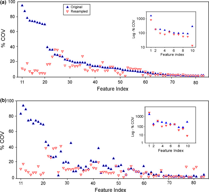
Absolute value of the %COV calculated from 116 original (solid triangles) and resampled (open triangles) image sets for 83 non‐wavelet features. Group 1 features that had %COV >50 after resampling are shown in the insets. Features are ordered (Feature Index) on the x‐axis from largest to lowest %COV value based on the images of the rubber cartridge, same order as in Table 2. The feature order for (a) rubber cartridge was applied to (b) ABS20 cartridge. [Colour figure can be viewed at wileyonlinelibrary.com]
Table 2.
Grouping of 85 non‐wavelet features based on %COV values after voxel‐size resampling
| Group 1 (%COV >50) | Group 3 Moderate (%COV <50) and negligible effect of resampling | |
|---|---|---|
| 1‐ NGTDM‐Busyness | 21‐ Fractal‐ SD | 53‐ GLCM‐Diff. Entropy |
| 2‐ GLSZM‐LISAE | 22‐ GLCM‐Info. Correlation1 | 54‐ GLCM‐Correlation |
| 3‐ GLSZM‐LILAE | 23‐ GLSZM‐SZV | 55‐ GLRLM‐LRHGE |
| 4‐ GLSZM‐IV | 24‐ GLRLM‐SRLGE | 56‐ GLCM‐ Autocorrelation |
| 5‐ GLSZM‐LIE | 25‐ GLRLM‐LGRE | 57‐ GLRLM‐HGRE |
| 6‐ GLSZM‐HILAE | 26‐ GLCM‐Kurtosis | 58‐ GLRLM‐SRHGE |
| 7‐ GLSZM‐LAE | 27‐ GLRLM‐LRLGE | 59‐ Fractal‐MeanLac3 |
| 8‐ GLSZM‐HISAE | 28‐ Fractal‐SDlac3 | 60‐ Intensity‐Uniformity |
| 9‐ GLSZM‐SAE | 29‐ GLCM‐Cluster prominence | 61‐ Intensity‐MaxI |
| 30‐ Fractal‐SDlac1 | 62‐ Fractal‐MeanLac2 | |
| Group 2 (%COV <30) | 31‐ GLCM‐Contrast | 63‐ GLCM‐Sum Average |
| 10‐ GLCM‐Variance | 32‐ Intensity‐SD | 64‐ Shape‐Convexity |
| 11‐ NGTDM‐ Coarseness | 33‐ Intensity‐Coeff. Vari. | 65‐ Fractal‐Mean FD |
| 12‐ GLCM‐Inverse variance | 34‐ Fractal‐SDlac2 (Table S1) | 66‐ Shape‐V(cc) |
| 13‐ NGTDM‐Texture Strength | 35‐ GLCM‐Difference Average | 67‐ GLRLM‐LRE |
| 14‐ Intensity‐Icl. homogeneity | 36‐ NGTDM‐Contrast | 68‐ GLRLM‐RPC |
| 15‐ GLCM‐Mean | 37‐ GLCM‐Info Correlation2 | 69‐ Shape‐Surf A(cm2) |
| 16‐ Intensity‐Contrast | 38‐ NGTDM‐ Complexity | 70‐ GLCM‐Sum Entropy |
| 17‐ GLRLM‐GLNU | 39‐ GLCM‐Inverse Variance P | 71‐ GLCM‐Entropy |
| 18‐ Intensity‐TGV | 40‐ GLSZM‐HIE | 72‐ Shape‐Surf/vol |
| 19‐ GLRLM‐RLNU | 41‐ GLCM‐Local homogeneity | 73‐ Shape‐Compactness |
| 20‐ Intensity‐ Energy | 42‐ GLCM‐Energy | 74‐ GLCM‐Inverse diff. |
| 43‐ GLCM‐Difference Variance | 75‐ Shape‐Long(mm) | |
| 44‐ Shape‐Short(mm) | 76‐ Intensity‐Hist. Entropy | |
| 45‐ Shape‐Eccentricity | 77‐ Intensity‐PeakI | |
| 46‐ GLCM‐Cluster tendency | 78‐ Shape‐Sphericity | |
| 47‐ GLCM‐Sum Variance | 79‐ Shape‐Sph. disprop. | |
| 48‐ GLCM‐Dissimilarity | 80‐ Intensity‐RMS | |
| 49‐ GLSZM‐ZP | 81‐ Intensity‐MeanI | |
| 50‐ Fractal‐MeanLac1 | 82‐ GLRLM‐SRE | |
| 51‐ GLCM‐Homogeneity1 | 83‐ GLCM‐Inverse diff. moment | |
| 52‐ Intensity‐Entropy | ||
| 84‐ Intensity‐MinI (not plotted) | ||
| 85‐ Intensity‐ Skewness (not plotted) | ||
The variability of the 83 features extracted from the rubber cartridge images with Ng = 8, 16, and 32 were compared with those extracted using Ng = 64 (Figure S1). The %COV values extracted from the original and resampled image sets were similar for all 83 features for Ng = 32 and 64 (Figure S1a). Similar results were obtained when comparing variability for Ng = 64 to Ng = 16 and 8 (Figures S1b and S1c), which showed similar %COV values except for several GLSZM features, namely, Intensity Variability (IV), Short Area Emphasis (SAE), Large Area Emphasis (LAE), and High Intensity Large Area Emphasis (HILAE) in group 1 (Table 2). These GLSZM features showed %COV values lower than 50% after resampling. Therefore, voxel‐size resampling did have a noticeable effect on some of the GLSZM features. The resampling effect at the lower number of gray levels, Ng = 8 and 16 for these features is readily observable (Figure S2).
The wavelet features derived from the first‐order statistics for the rubber and ABS20 cartridges are shown in Figs. 2a and 2b respectively. First‐order energy, contrast, TGV and local homogeneity derived from 8 different wavelet decompositions improved significantly after resampling for both cartridges. The only exception was for local homogeneity (LLH), which showed large variation even after resampling (group 1, Table 3). Most skewness combinations for the rubber cartridge and most kurtosis decompositions for ABS20 cartridge had large variability before and after resampling. Sixty eight percent of the wavelet features were found to be reproducible across voxel sizes, and therefore, resampling had negligible effect on these features. The %COV values for 128 wavelet features extracted using lower number of gray levels Ng = 8, 16, and 32 were in agreement with results obtained for Ng = 64. For wavelet features, comparisons of all four gray levels, Ng = 8, 16, 32, and 64, after resampling are shown in Figure S3.
Figure 2.
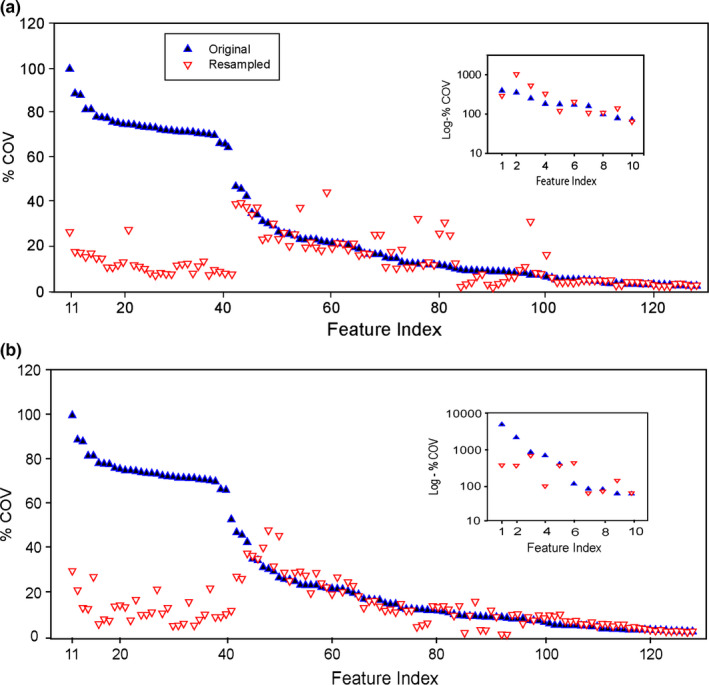
Absolute value of the %COV calculated from 72 original (solid triangles) and resampled (open triangles) image sets for 128 wavelet features. Group 1 features that had %COV >50 after resampling are shown in the insets. Features are ordered (Feature index) on the x‐axis from largest to lowest %COV value. Different feature order was used for (a) rubber cartridge and (b) ABS20 cartridge. [Colour figure can be viewed at wileyonlinelibrary.com]
Table 3.
Grouping of 128 first‐order wavelet features based on %COV values after resampling
| Group 1 (%COV >50) (10/128) features each cartridge | Group 2 (%COV <30) (31/128) features each cartridge | Group 3 Moderate (%COV <50) (87/128) features each cartridge | ||
|---|---|---|---|---|
| Rubber Cartridge | ABS20 Cartridge | Rubber & ABS20 (All Filter Combinations) | Rubber Cartridge (All Filter Combinations) | ABS20 Cartridge (All Filter Combinations) |
| Skewness (All filter combinations) | Kurtosis (All filter combinations) Except LLH & HHH | Local Homogeneity (Except LLH lcl. homo) | Kurtosis‐ (all combinations except HHH‐ Kurtosis) | Skewness‐ (all combinations except LHH, HLH, HHH‐ Skewness) |
| Lcl. homo (LLH) | Lcl. homo (LLH) | TGV | Min. I | Kurtosis (HHH) |
| Kurtosis (HHH) | Skewness (LHH) | Energy | Max. I | Kurtosis (LLH) |
| Skewness (HLH) | Contrast | Peak I | Min. I, Max. I | |
| Skewness (HHH) | Mean I | Peak I, Mean I | ||
| Hist. Entropy | Hist. Entropy | |||
| Uniformity | Uniformity | |||
| Coeff. Vari. | Coeff. Vari | |||
| Entropy | Entropy | |||
| S.D. | S.D. | |||
| RMS | RMS | |||
3.B. Normalization by voxel size
Identified feature values calculated using the original and normalized feature definitions are plotted as a function of pixel size and slice thickness in Fig. 3 (also Figure S4). Feature values were scaled before plotting to obtain a similar range of values for all features. The same ROIs as for voxel resampling were used here. After feature modifications, energy, TGV, entropy from first‐order statistics, mean and inverse variance from GLCM, and RLNU and GLNU from GLRLM were found to be reproducible across the studied voxel volumes. Variations in modified coarseness and texture strength were relatively larger but median values were similar for all pixel sizes. Contrast from GLCM indicated high variations even after feature modifications (Figure S4). Notice that entropy from first‐order statistics was normalized using the logarithm of the number of voxels in the ROI. The results were similar across all ROI sizes. The normalizing factors for the identified features are shown in Table 4.
Figure 3.

Scaled features values extracted from original and normalized feature definitions as a function of pixel size and slice thickness. Modified values are shown by box plot. Middle, lower and upper lines in the box indicate median, first quartile, and third quartile respectively. Energy (a) from intensity histogram and GLNU (b) from the GLRLM almost converge to a straight horizontal line after normalization. Coarseness (c) and texture strength (d) from NGTDM exhibit small variations in median values, but with small dependence on slice thickness and pixel spacing after normalization.
Table 4.
Ten radiomics features from different feature groups that were normalized using voxel size
| Feature | Description | Original Feature formula f(P,T) | Modified Feature formula | |||
|---|---|---|---|---|---|---|
| First‐order features based on Intensity Histogram | ||||||
| 20‐ Energy | Measures homogeneity of intensity histogram |
|
|
|||
| 52‐ Entropy | Measure of disorder |
|
|
|||
| 18‐ TGV | Total summed intensity in ROI |
|
V(P,T) * f(P,T) | |||
| 16‐ Contrast | Intensity variation of intensity histogram |
|
V(P,T) * f(P,T) | |||
| Second order features based on Co‐occurrence matrix | ||||||
| 12‐ Inverse Variance | Place low weight on values differing from average matrix value |
|
V(P,T) * f(P,T) | |||
| 15‐ Mean | The mean value of the co‐occurrence matrix |
|
V(P,T) * f(P,T) | |||
| Gray‐level run‐length matrix (RLM) features | ||||||
| 17‐ GLNU | Measures the non‐uniformity of the gray levels |
|
V(P,T) * f(P,T) | |||
| 19‐ RLNU | Measure the non‐uniformity of the run lengths |
|
V(P,T) * f(P,T) | |||
| Gray‐level Neighborhood Difference Matrix (NGTDM) | ||||||
| 11‐ Coarseness | Measure of texture uniformity |
|
|
|||
| 13‐ Texture Strength | Measure of distinguishability between clusters of different intensities. |
|
|
|||
V (P, T), n (P, T) are described in text. T (x, y, z) is the normalized value obtained from each voxel. T (i) is the probability of the occurrence of the gray‐level i and Ng is the number of discrete intensity levels. I (v) is the intensity of a voxel, G is the number of voxels in a volume‐of‐interest (VOI). Other terminology used for GLCM, GLRLM, and NGTDM features is described in Table 5 and Table 6. Feature number is given according to Table 2.
Interscanner comparison using voxel‐size normalization for identified features for the rubber cartridge are shown in Fig. 4 (Figure S5). The normalized feature values in each case form a horizontal straight line, thereby indicating that the normalized features were reproducible across different scanners. Non‐normalized feature values for the two Philips and the four Siemens scanners were in close agreement, but not so for the two GE scanners; this is because the GE scanners differed in slice thicknesses, and thus in voxel size. Exceptions were contrast from GLCM and texture strength from NGTDM (Figure S5) for which both GE scanners produced results that were different from the other 6 scanners even after feature normalization.
Figure 4.
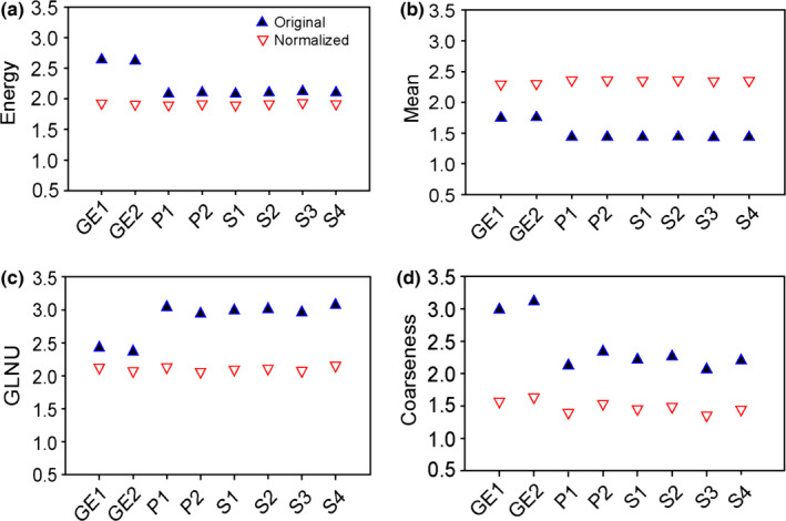
Scaled original (solid triangles) and normalized (open triangles) features values across 8 different scanners: Normalized values for energy (a) from intensity histogram, mean (b) from GLCM, GLNU (c) from GLRLM, and coarseness (d) from NGTDM nearly converge into horizontal straight lines for all scanners, while the original feature values for two GE scanners were different because of different slice thickness. [Colour figure can be viewed at wileyonlinelibrary.com]
3.C. Normalization by number of gray levels
Only 7 out of 51 texture features, namely, Inverse difference moment (IDM), inverse difference (ID), information correlation 1 and information correlation 2 from GLCM; short run emphasis (SRE) and run percentage (RPC) from GLRLM; and coarseness from NGTDM, were found reproducible (%COV <20) with varying gray‐level discretization for all phantom materials. The remaining 44 features had large variation with discretization (%COV >20). Most of the remaining 44 features were dependent on the number of gray levels. For some features, their relationship with gray levels appeared to be random, therefore, no normalizing factor could be identified. However, 17 out of 44 features showed a trend with varying number of gray levels. Further investigation indicated that these feature had linear, quadratic and cubic type relationships with the number of gray levels. These dependencies were minimized or eliminated by introducing the normalizing factors given in Table 5 and Table 6.
Table 5.
GLCM features normalized by the number of gray levels
| Feature | Original Feature formula f | Modified Feature formula fm | ||
|---|---|---|---|---|
| 71‐ Entropy |
|
|
||
| 53‐ Diff. Entropy |
|
|
||
| 70‐ Sum Entropy |
|
|
||
| 31‐ Contrast |
|
|
||
| 15‐ Mean |
|
f * Ng* Ng | ||
| 47‐ Sum Variance |
|
|
||
| 43‐ Difference Variance |
|
|
||
| 63‐ Sum Average |
|
|
||
| 35‐ Difference Average |
|
|
||
| 48‐ Dissimilarity |
|
|
p (i, j) is the co‐occurrence matrix. Ng is the number of discrete gray levels. px is the ith entry obtained by summing the rows of p (i, j), py is the jth entry obtained by summing the columns of p(i, j). Feature number is given according to Table 2.
Table 6.
GLRLM, GLSZM, and NGTDM features normalized by the number of gray levels
| Feature | Original Feature formula f | Modified Feature formula, fm | |||
|---|---|---|---|---|---|
| Gray‐level run‐length matrix (GLRLM) features | |||||
| 17‐ GLNU |
|
f * Ng | |||
| 57‐ HGRE |
|
|
|||
| 58‐ SRHGE |
|
|
|||
| Neighborhood gray tone difference matrix (NGTDM) features | |||||
| 36‐ Contrast |
|
|
|||
| 38‐ Complexity |
|
|
|||
| 13‐ Texture strength |
|
|
|||
| Gray‐level size zone matrix (GLSZM) feature | |||||
| 40‐ HIE |
|
|
|||
a‐ GLRLM: R (i, j) is the (i, j)th entry in the given run‐length matrix and Ng is the number of discrete gray levels in the image. M is the longest run and n is the number of pixels in the image.
b‐ NGTDM: Pi is the probability of occurrence of voxel of intensity i and M (i) is the NGTDM value of intensity i. Nh is the highest gray‐level value and Ng is the number of gray levels present in the image.
c‐ GLSZM: In size zone matrix z (i, j), rows i indicate gray levels and columns indicating zone sizes. Ng is the number of gray levels and the largest zone size is indicated by m. Ω is the total number of unique connected zones.
Feature number is given according to Table 2.
Original and normalized feature values as function of number of gray levels for contrast and dissimilarity from GLCM for rubber and ABS20 cartridges are shown in Fig. 5. The mean value of %COV decreased to below 20% for all 17 texture features after normalization as shown in the Fig. 6. The normalizing factors were tested for different‐sized ROIs encompassing the rubber and ABS20 cartridges that resulted in reproducible feature values. Most of GLSZM features and busyness from NGTDM were found to have large variation with the number of gray levels.
Figure 5.
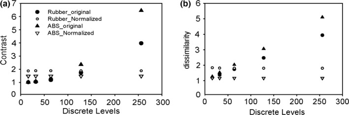
Scaled original and normalized feature values as function of number of gray levels (Ng) for rubber and ABS20 cartridges: Contrast (a) and dissimilarity (b) from GLCM became independent of Ng after gray‐level normalization as shown by open triangles and circles.
Figure 6.
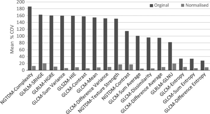
The %COV calculated over 12 different ROIs (10 ROIs of 14 cm3 for each of the 10 cartridges in the phantom and 2 larger ROIs of 50 and 60 cm3 contoured over multiple cartridges, i.e., ABS, wood and shredded rubber before (dark bars) and after (light bars) normalization. The phantom was scanned with a Siemens Definition AS scanner with pixel size of 0.48 mm and slice thickness of 3 mm.
4. Discussion
A necessary property of a radiomic feature to qualify as a potential imaging biomarker is robustness, for example, insensitivity to data acquisition and image reconstruction settings. Recent studies however, show that many features exhibit large variability because of acquisition and reconstruction parameters.14, 36 In routine CT diagnostic studies, there is large variability in slice thickness and pixel spacing of the images because of user preference, protocol requirements, manufacturer's settings, etc. These two parameters determine the voxel size, i.e., the image spatial resolution. Therefore, evaluating the impact of voxel size on CT radiomic features is of paramount importance. Most features were initially developed for non‐medical applications and for planar images. Consequently, original formulas and algorithms to compute feature values may have made assumptions that may not be applicable to modern medical images. Voxel‐size resampling or voxel‐size normalization might be required for some features in the case of 3D medical image sets reconstructed using a range of voxel sizes. In this phantom study, we found 30% of the features were highly sensitive to voxel size. For the voxel size‐dependent features, we presented two methods to improve the robustness of the features among images reconstructed with different voxel sizes: one method was to resample all images to a chosen voxel size, and the other method was to normalize feature values by voxel size.
Resampling of CT phantom image sets to uniform voxel size increased the robustness of 42 out of 213 features studied. These were: 4 features from first‐order statistics, 3 features from GLCM, 2 features from GLRLM, 2 features from NGTDM, and 31 wavelet features (e.g., energy, local homogeneity, TGV, contrast) derived from the first‐order statistics of the 8 different image decompositions from each ROI. Not surprisingly, the behavior of some wavelet features with voxel‐size resampling was similar to that of first‐order features derived from the intensity histograms. Interestingly, some features such as run‐length‐based GLNU and coarseness from NGTDM were identified as promising features in recent studies. For example, coarseness, which resembles human perception of image granularity, was found to be clinically useful in differentiating head and neck tumors and lymph nodes from normal tissues.37 This feature was also found to be a useful biomarker in predicting response of chemotherapy in case of non‐small cell lung cancer38 and esophageal cancer.8 Gray‐level non‐uniformity from GLRLM was found to have intermediate variations because of FDG‐PET acquisition and reconstruction parameters,12 in contrast to our results that indicated large dependency on voxel size. In the same study,12 coarseness from NGTDM exhibited large variability in close agreement with our results. The large variability in feature values was greatly reduced after resampling, thereby suggesting resampling of all image sets to the a pre‐selected voxel size as a way to eliminate dependencies introduced by voxel volume or the number of voxels in the ROI.
The voxel size of a CT image can be changed by resampling the slice thickness along the longitudinal z‐axis or by resampling pixel size in the axial (x‐y) plane. We found 10 features that were intrinsically dependent on voxel size. Therefore, incorporating voxel size in the definitions of these identified features improved their robustness as shown in Fig. 3 (and Figure S4). These results were in agreement with a recent study39 for Intensity‐energy, NGTDM‐Coarseness, GLRLM‐GLNU and GLRLM‐RLNU, but not for busyness from NGTDM which showed large variability before and after normalization. Additionally, we identified more features, namely, Intensity‐entropy, Intensity‐contrast, GLCM‐mean, and NGTDM‐Texture strength that were dependent on voxel size. A cautionary point to make here is that features are not standardized, and therefore, features with the similar names may have different definitions/algorithms in different publications.40 Therefore, standardization of feature names, mathematical definitions, and implementation algorithms is needed.
Imaging data for radiomics studies typically originate from multiple scanners, therefore, radiomic features that are robust across scanners would be desirable. In this study, we showed that features normalized by voxel size were robust across scanners. Without normalization, the identified features behaved similarly for images from Siemens and Philips scanners, but not for GE scanners (Fig. 4). This was a consequence of the GE detector design which restricted slice thickness values; therefore, voxel size was the reason for the difference seen in GE scanners. This also explains the dependence of some radiomics features on scanner manufacturer in a recent study15 in which phantom scans were resampled to in‐plane pixel spacing of 1 mm,2 but slice thicknesses ranged from 2 to 3 mm.
Therefore, without normalization or voxel‐size resampling, the identified features convey information related to the volume of the ROI predominantly, and not to texture or other intervoxel relationships. To ensure meaningful results, we recommend researchers perform voxel‐size normalization for these voxel‐size‐dependent features and resampling for all features. Resampling of all images to a particular voxel size should be done for standardization because non‐voxel‐size‐dependent features may have different values for different voxel sizes independently of ROI volume.
In a separate analysis, only 7 out of 51 texture features were found to be robust with respect to varying number of gray levels. These findings were partly in agreement with a recent study41 for features such as coarseness, Info correlation (1), inverse difference and inverse difference moment. However, we found variability (i.e., %COV >20) for other features such as difference entropy, sum entropy, entropy, variance, homogeneity 1 and homogeneity 2 in contrast to the same study. We identified 17 texture features that were dependent on Ng; normalizing these features by the number of gray levels increased their robustness (Fig. 6). It is possible that for a given Ng, a texture feature may be robust. Therefore, large variability as a function of gray‐level discretization does not necessarily imply a feature is useless for clinical applications.
Currently, there is lack of standardization regarding the feature extracting methodology.23 Different radiomics groups have used different methodologies, such as different number of gray levels to extract features. As shown by recent studies,23, 41 texture features may be highly correlated with Ng. In this study, we tried to identify normalizing factors for these features to minimize or eliminate their dependencies on Ng. These dependencies are in fact expected from the equations that define the features, but what has not been made clear is, first, the existence of these intrinsic dependencies, and second, how the intrinsic dependencies can be minimized or eliminated. This is important to eventually be able to compare features in multicenter studies and clinical trials. Otherwise, a feature value for a given texture definition would be different across institutions because of differences in feature extraction methods. Moreover, there may be advantages or disadvantages in using features with or without dependencies on the number of gray levels. A more general approach would be to consider features computed with different number of gray levels as different features altogether, that is, the number of gray levels are part of the feature definitions. The main import here is that feature may have Ng‐dependencies, and these dependencies may lead to poor or erroneous conclusions if one is unaware.
Gray‐level resampling only affects second and higher order radiomics features. However, voxel‐size variation could impact both first, second and higher order features. Identification of texture features that depend on the number of gray levels and/or the voxel size is necessary to remove or reduce the intrinsic dependencies from feature definitions. For example, coarseness was a feature that showed large variability with voxel size but robustness with gray‐level; hence only normalization by voxel volume (or number of voxels) would be required. Other features such as GLNU, mean and texture strength were sensitive to both voxel size and number of gray levels, therefore, they would require normalization by voxel size as well as the number of gray levels.
Finally, a limitation of this study was that we used a texture phantom;15 therefore biological correlation for identified features was not addressed. However, stable texture phantoms are advantageous since they provide stable geometry and physical characteristics for testing the robustness of CT radiomic features; a prerequisite for studies with human subjects. Moreover, interscanner, intrascanner, and multicenter variability in CT radiomic features because of acquisition and reconstruction parameters can be more readily assessed with phantoms.
5. Conclusions
In this study, we identified 42 out of 213 features that were dependent on voxel size. This dependency can be removed either by resampling all the image sets to a nominal voxel size, as described in this paper, or by normalizing by voxel size. Either approach is a recommended pre‐processing step before feature extraction. Moreover, 17 texture features were dependent on the number of gray levels. This dependency can also be removed or reduced by normalizing by the number of gray levels used. These findings suggest that feature definitions must be revisited to remove these and perhaps other dependencies introduced when they were first reported.
Conflict of interest
None declared.
Supporting information
Figure S1: Comparison of 83 features extracted from original and resampled data with Ng = 64 to those same features extracted with lower number of gray levels. Comparison of Ng = 64 to (a) Ng = 32, (b) Ng = 16, and to (c) Ng = 8. Features indicated similar trend at Ng = 32, 16, and 8 as did for Ng = 64 except for 4 GLSZM features which showed %COV <50 after resampling at Ng = 8 and 16 as shown in the inset of panels b and c.
Figure S2: Comparison of group 1 (Table 2 in manuscript) GLSZM features for Ng = 8, 16, 32, and 64 after voxel‐size resampling. Four GLSZM features, namely, IV, LAE, SAE, and HISAE showed %COV <50 for Ng = 8 and Ng = 16.
Figure S3: Comparisons of first‐order wavelets for Ng = 8, 16, 32, and 64 after voxel‐size resampling. For group 1 features (Table 2I in manuscript), %COV >50 for all gray levels as shown in the inset. The %COV <30 for group 2 features (features 11 to 41 in Table 3 in the manuscript) and % COV <50 for group 3 (features 42–128 in Table 3 in the manuscript) for all Ng values.
Figure S4: Scaled features values extracted from original and voxel‐size normalized feature definitions as a function of pixel size and slice thickness. Modified values are shown in box plots. Middle, lower, and upper lines in the box indicate the median, first quartile and third quartile respectively. The Mean (a) and Inverse Variance (f) from GLCM; TGV (b) and Entropy (c) from intensity histogram; and RLNU (d) from GLRLM all converge into a straight horizontal line after voxel‐size normalization. Contrast (e) from intensity histogram showed large variability but its median value was pretty constant for all voxel sizes.
Figure S5: Scaled original (solid triangles) and voxel‐size normalized (open triangles) feature values as a function of 8 different scanners for the rubber cartridge: Normalized values for TGV (b) and Entropy (f) from intensity histogram; RLNU (e) from RLM; and Inverse Variance (d) from GLCM all nearly converge into straight horizontal line for all scanners. Normalized and original values for Texture Strength (c) from NGTDM and Contrast (a) from Intensity histogram were similar for 6 scanners but different for GE scanners. The reason for this difference were the restrictions on slice thicknesses by the GE scanners used.
Table S1: Acronyms used in this study.
Table S2: Shape and Intensity histogram features.
Table S3: GLCM features.
Table S4: GLSZM, GLRLM, and NGTDM features.
Data S1: Description of radiomics features.
Acknowledgments
We would like to acknowledge Rich Guzman and Robert Sander for their assistance in acquiring phantom scans on different CT scanners at Moffitt cancer center main campus and Moffitt international plaza. This project was partly supported by NIH/NCI funding ROICA190105‐01.
References
- 1. Lambin P, Rios‐Velazquez E, Leijenaar R, et al. Radiomics: Extracting more information from medical images using advanced feature analysis. Eur J Cancer. 2012;48:441–446. [DOI] [PMC free article] [PubMed] [Google Scholar]
- 2. Gillies RJ, Anderson AR, Gatenby RA, Morse DL. The biology underlying molecular imaging in oncology: From genome to anatome and back again. Clin Radiol. 2010;65:517–521. [DOI] [PMC free article] [PubMed] [Google Scholar]
- 3. Aerts HJWL, Velazquez ER, Leijenaar RTH, et al. Decoding tumour phenotype by noninvasive imaging using a quantitative radiomics approach. Nat Commun. 2014;5:4006–4013. [DOI] [PMC free article] [PubMed] [Google Scholar]
- 4. Kuo MD, Gollub J, Sirlin CB, Ooi C, Chen X. Radiogenomic analysis to identify imaging phenotypes associated with drug response gene expression programs in hepatocellular carcinoma. J Vasc Interv Radiol. 2007;18:821–830. [DOI] [PubMed] [Google Scholar]
- 5. Lee H‐J, Kim YT, Kang CH, et al. Epidermal growth factor receptor mutation in lung adenocarcinomas: Relationship with CT characteristics and histologic subtypes. Radiology. 2013;268:254–264. [DOI] [PubMed] [Google Scholar]
- 6. Karlo CA, Paolo PLD, Chaim J, et al. Radiogenomics of clear cell renal cell carcinoma: Associations between CT imaging features and mutations. Radiology. 2014;270:464–471. [DOI] [PMC free article] [PubMed] [Google Scholar]
- 7. Gevaert O, Xu J, Hoang CD, et al. Non–small cell lung cancer: Identifying prognostic imaging biomarkers by leveraging public gene expression microarray data—methods and preliminary results. Radiology. 2012;264:387–396. [DOI] [PMC free article] [PubMed] [Google Scholar]
- 8. Tixier F, Le Rest CC, Hatt M, et al. Intratumor heterogeneity characterized by textural features on baseline 18F‐FDG PET images predicts response to concomitant radiochemotherapy in esophageal cancer. J Nucl Med. 2011;52:369–378. [DOI] [PMC free article] [PubMed] [Google Scholar]
- 9. Coroller TP, Grossmann P, Hou Y, et al. CT‐based radiomic signature predicts distant metastasis in lung adenocarcinoma. Radiother Oncol 2015;114:345–350. [DOI] [PMC free article] [PubMed] [Google Scholar]
- 10. Kumar V, Gu Y, Basu S, et al. Radiomics: The process and the challenges. Magn Reson Imaging. 2012;30:1234–1248. [DOI] [PMC free article] [PubMed] [Google Scholar]
- 11. Zhao B, Tan Y, Tsai W‐Y, et al. Reproducibility of radiomics for deciphering tumor phenotype with imaging. Sci Rep. 2016;6:23428. [DOI] [PMC free article] [PubMed] [Google Scholar]
- 12. Galavis PE, Hollensen C, Jallow N, Paliwal B, Jeraj R. Variability of textural features in FDG PET images due to different acquisition modes and reconstruction parameters. Acta Oncol (Stockholm, Sweden). 2010;49:1012–1016. [DOI] [PMC free article] [PubMed] [Google Scholar]
- 13. Ganeshan B, Miles KA. Quantifying tumour heterogeneity with CT. Cancer imaging. 2013;13:140–149. [DOI] [PMC free article] [PubMed] [Google Scholar]
- 14. Nyflot MJ, Yang F, Byrd D, Bowen SR, Sandison GA, Kinahan PE. Quantitative radiomics: Impact of stochastic effects on textural feature analysis implies the need for standards. J Med Imaging (Bellingham, Wash.). 2015;2:041002. [DOI] [PMC free article] [PubMed] [Google Scholar]
- 15. Mackin D, Fave X, Zhang L, et al. Measuring computed tomography scanner variability of radiomics features. Invest Radiol. 2015;50:757–765. [DOI] [PMC free article] [PubMed] [Google Scholar]
- 16. Fave X, Mackin D, Yang J, et al. Can radiomics features be reproducibly measured from CBCT images for patients with non‐small cell lung cancer? Med Phys. 2015;42:6784–6797. [DOI] [PMC free article] [PubMed] [Google Scholar]
- 17. Basu S, Hall LO, Goldgof DB, et al. Developing a classifier model for lung tumors in CT‐scan images. I. E. International Conference on Systems, Man, and Cybernetics (SMC), IEEE. 2011;1306–1312.
- 18. Zhao B, Tan Y, Tsai WY, Schwartz LH, Lu L. Exploring variability in CT characterization of tumors: A preliminary phantom study. Transl Oncol. 2014;7:88–93. [DOI] [PMC free article] [PubMed] [Google Scholar]
- 19. Yip SS, Aerts HJ. Applications and limitations of radiomics. Phys Med Biol. 2016;61:R150–R166. [DOI] [PMC free article] [PubMed] [Google Scholar]
- 20. El Naqa I, Grigsby P, Apte A, et al. Exploring feature‐based approaches in PET images for predicting cancer treatment outcomes. Pattern Recogn. 2009;42:1162–1171. [DOI] [PMC free article] [PubMed] [Google Scholar]
- 21. Vaidya M, Creach KM, Frye J, Dehdashti F, Bradley JD, El Naqa I. Combined PET/CT image characteristics for radiotherapy tumor response in lung cancer. Radiother Oncol. 2012;102:239–245. [DOI] [PubMed] [Google Scholar]
- 22. Hatt M, Tixier F, Cheze Le Rest C, Pradier O, Visvikis D. Robustness of intratumour (1)(8)F‐FDG PET uptake heterogeneity quantification for therapy response prediction in oesophageal carcinoma. Eur J Nucl Med Mol Imaging. 2013;40:1662–1671. [DOI] [PubMed] [Google Scholar]
- 23. Leijenaar RT, Nalbantov G, Carvalho S, et al. The effect of SUV discretization in quantitative FDG‐PET Radiomics: The need for standardized methodology in tumor texture analysis. Sci Rep. 2015;5:11075. [DOI] [PMC free article] [PubMed] [Google Scholar]
- 24. Haralick RM, Shanmugam K, Dinstein I. Textural features for image classification. IEEE Trans Syst Man Cybern. 1973;3:610–621. [Google Scholar]
- 25. Haralick RM. Statistical and structural approaches to texture. Proc IEEE. 1979;67:786–804. [Google Scholar]
- 26. O JA, Aborisade DO, Amole AO, Durodola AO. Comparative analysis of textural features derived from GLCM for ultrasound liver image classification. Int J Comput Trends Technol. 2014;V11:239–244. [Google Scholar]
- 27. Kurani AS, Xu D‐H, Furst J, Raicu DS. Presented at the 7th IASTED International Conference on Computer Graphics and Imaging, Kauai, Hawaii‐USA, CGIM; 2004.
- 28. Oliver JA, Budzevich M, Zhang GG, Dilling TJ, Latifi K, Moros EG. Variability of image features computed from conventional and respiratory‐gated PET/CT images of lung cancer. Trans Oncol. 2015;8:524–534. [DOI] [PMC free article] [PubMed] [Google Scholar]
- 29. Galloway MM. Texture analysis using gray level run lengths. Comput Graph Image Process. 1975;4:172–179. [Google Scholar]
- 30. Chu A, Sehgal CM, Greenleaf JF. Use of gray value distribution of run lengths for texture analysis. Pattern Recogn Lett. 1990;11:415–419. [Google Scholar]
- 31. Dasarathy BV, Holder EB. Image characterizations based on joint gray level—run length distributions. Pattern Recogn Lett. 1991;12:497–502. [Google Scholar]
- 32. Thibault G, Fertil B, Navarro C, et al. Texture indexes and gray level size zone matrix application to cell nuclei classification. 10th International Conference on Pattern Recognition and Information Processing. 2009.
- 33. Amadasun M, King R. Textural features corresponding to textural properties. IEEE Trans Syst Man Cybern. 1989;19:1264–1274. [Google Scholar]
- 34. Sarkar N, Chaudhuri BB. An efficient approach to estimate fractal dimension of textural images. Pattern Recogn. 1992;25:1035–1041. [Google Scholar]
- 35. Jin XC, Ong SH, Jayasooriah. A practical method for estimating fractal dimension. Pattern Recogn Lett. 1995;16:457–464. [Google Scholar]
- 36. Hunter LA, Krafft S, Stingo F, et al. High quality machine‐robust image features: Identification in nonsmall cell lung cancer computed tomography images. Med Phys. 2013;40:121916. [DOI] [PMC free article] [PubMed] [Google Scholar]
- 37. Yu H, Caldwell C, Mah K, Mozeg D. Coregistered FDG PET/CT‐based textural characterization of head and neck cancer for radiation treatment planning. IEEE Trans Med Imaging. 2009;28:374–383. [DOI] [PubMed] [Google Scholar]
- 38. Cook GJR, Yip C, Siddique M, et al. Are pretreatment 18F‐FDG PET tumor textural features in non‐small cell lung cancer associated with response and survival after chemoradiotherapy? J Nucl Med. 2013;54:19–26. [DOI] [PubMed] [Google Scholar]
- 39. Fave X, Zhang L, Yang J, et al. Impact of image preprocessing on the volume dependence and prognostic potential of radiomics features in non‐small cell lung cancer. Trans Cancer Res. 2016;5:349–363. [Google Scholar]
- 40. Brooks FJ. On some misconceptions about tumor heterogeneity quantification. Eur J Nucl Med Mol Imaging. 2013;40:1292–1294. [DOI] [PubMed] [Google Scholar]
- 41. Lu L, Lv W, Jiang J, et al. Robustness of radiomic features in [11C]choline and [18F]FDG PET/CT imaging of nasopharyngeal carcinoma: Impact of segmentation and discretization. Mol Imaging Biol. 2016;18:935–945. [DOI] [PubMed] [Google Scholar]
Associated Data
This section collects any data citations, data availability statements, or supplementary materials included in this article.
Supplementary Materials
Figure S1: Comparison of 83 features extracted from original and resampled data with Ng = 64 to those same features extracted with lower number of gray levels. Comparison of Ng = 64 to (a) Ng = 32, (b) Ng = 16, and to (c) Ng = 8. Features indicated similar trend at Ng = 32, 16, and 8 as did for Ng = 64 except for 4 GLSZM features which showed %COV <50 after resampling at Ng = 8 and 16 as shown in the inset of panels b and c.
Figure S2: Comparison of group 1 (Table 2 in manuscript) GLSZM features for Ng = 8, 16, 32, and 64 after voxel‐size resampling. Four GLSZM features, namely, IV, LAE, SAE, and HISAE showed %COV <50 for Ng = 8 and Ng = 16.
Figure S3: Comparisons of first‐order wavelets for Ng = 8, 16, 32, and 64 after voxel‐size resampling. For group 1 features (Table 2I in manuscript), %COV >50 for all gray levels as shown in the inset. The %COV <30 for group 2 features (features 11 to 41 in Table 3 in the manuscript) and % COV <50 for group 3 (features 42–128 in Table 3 in the manuscript) for all Ng values.
Figure S4: Scaled features values extracted from original and voxel‐size normalized feature definitions as a function of pixel size and slice thickness. Modified values are shown in box plots. Middle, lower, and upper lines in the box indicate the median, first quartile and third quartile respectively. The Mean (a) and Inverse Variance (f) from GLCM; TGV (b) and Entropy (c) from intensity histogram; and RLNU (d) from GLRLM all converge into a straight horizontal line after voxel‐size normalization. Contrast (e) from intensity histogram showed large variability but its median value was pretty constant for all voxel sizes.
Figure S5: Scaled original (solid triangles) and voxel‐size normalized (open triangles) feature values as a function of 8 different scanners for the rubber cartridge: Normalized values for TGV (b) and Entropy (f) from intensity histogram; RLNU (e) from RLM; and Inverse Variance (d) from GLCM all nearly converge into straight horizontal line for all scanners. Normalized and original values for Texture Strength (c) from NGTDM and Contrast (a) from Intensity histogram were similar for 6 scanners but different for GE scanners. The reason for this difference were the restrictions on slice thicknesses by the GE scanners used.
Table S1: Acronyms used in this study.
Table S2: Shape and Intensity histogram features.
Table S3: GLCM features.
Table S4: GLSZM, GLRLM, and NGTDM features.
Data S1: Description of radiomics features.