Numerical Interpretation of Molecular Surface Field in Dielectric Modeling of Solvation

Abstract

Continuum solvent models, particularly those based on the Poisson-Boltzmann equation (PBE), are widely used in the studies of biomolecular structures and functions. Existing PBE developments have been mainly focused on how to obtain more accurate and/or more efficient numerical potentials and energies. However to adopt the PBE models for molecular dynamics simulations, a difficulty is how to interpret dielectric boundary forces accurately and efficiently for robust dynamics simulations. This study documents the implementation and analysis of a range of standard fitting schemes, including both one-sided and two-sided methods with both first-order and second-order Taylor expansions, to calculate molecular surface electric fields to facilitate the numerical calculation of dielectric boundary forces. These efforts prompted us to develop an efficient approximated one-dimensional method, which is to fit the surface field one dimension at a time, for biomolecular applications without much compromise in accuracy. We also developed a surface-to-atom force partition scheme given a level set representation of analytical molecular surfaces to facilitate their applications to molecular simulations. Testing of these fitting methods in the dielectric boundary force calculations shows that the second-order methods, including the one-dimensional method, consistently perform among the best in the molecular test cases. Finally, the timing analysis shows the approximated one-dimensional method is far more efficient than standard second-order methods in the PBE force calculations.

Graphical Abstract

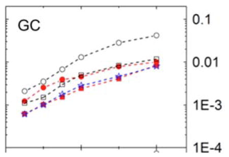
A semi-log plot of mean absolute errors of atomic dielectric boundary forces (kcal/mol-e-Å) versus grid spacing (tested from 1/16 Å to 1/2 Å) for a nucleic acid base pair with multiple surface field fitting methods: one-sided first-order (black circle), one-sided second-order (black square), two-sided first-order (red circle), two-sided second-order (red square), and finally the approximated one-dimensional method (blue star). Our analysis shows that the efficient one-dimensional method achieves similar accuracy as the more expensive second-order method but with a fraction of the computational cost.

Introduction

Solvation interaction is one of the essential determinants of the structures and functions in proteins and nucleic acids, and crucial in their high accuracy modeling.^[1–21] As most particles in a molecular model represent water molecules solvating the target biomolecules, treating these water molecules implicitly offers an opportunity to reach higher computational efficiency and/or to model more complex biomolecular systems. After years of basic research and development, implicit or continuum models of solvation interactions, specifically the electrostatic solvation modeling that is based on the Poisson-Boltzmann equation (PBE), are widely used in the studies of biomolecules.^[1–21] Indeed continuum electrostatics modeling represents a physically effective approach that makes it possible to account for a number of phenomena involving solvent electrostatic effects in functional analyses of biomolecules.^[1–21] These are facilitated by numerical solutions of the PBE that can be obtained routinely for biomolecules and their complexes.^[3,22–39]

In the continuum PBE solvent models, the solute region is treated as a low dielectric constant region and the solvent region is treated as a high dielectric constant region. A number of fixed interior point charges are located at atomic centers. As analytical solution of the PBE can be achieved only in a few specific cases with simple solute geometry, numerical solutions of the PBE are almost always needed for biomolecular applications. Among the numerical solution methods for PBE, finite-difference method (FDM),^{[23,24,27,32,33,36,38,40–50]} finite-element method,^[51–59] and boundary-element method ^[60–75] are mostly used. The PBE-based models have wide biological applications. For example, they have been applied to predictions of pKa values for ionizable groups in biomolecules,^{[ 76–81]} solvation free energies,^[82,83] binding free energies,^{[ 84–89]} and protein folding and design.^[90–98]

A difficulty in applying the numerical PBE methods is to incorporate these methods into molecular simulations, due to the difficulty in assigning dielectric boundary/molecular surface forces to solute atoms.^{[51,99–108]} Much effort has been devoted to improve methods to facilitate the use of the PBE models in molecular dynamics simulations.^{[51,65,99–118]} Gilson et al. presented a variational approach to compute the total electrostatic forces, with a special focus on numerical interpretation of the dielectric boundary forces (DBF).^[103] Che et al. proposed an alternative interpretation scheme for the discontinuous dielectric constant model via the variational principle.^[105] To enhance the numerical convergence and stability of DBFs, Cai et al. proposed a charge-based strategy.^{[ 106,108]} Starting from the Laudau and Lifshitz framework, Xiao et al. derived the Maxwell stress tensor for the full nonlinear PBE system to compute electrostatic forces for electrostatic systems with finite number of singularities, including point charges and discontinuous dielectric, with which a DBF formalism can also be derived for the discontinuous dielectric constant model.^[119]

Given these theoretical developments, we are ready to address their practical applications to molecular simulations. However, most numerical PBE solvers can only obtain electric potential and field readily at atomic centers, but all DBF algorithms require surface electric field as input. Furthermore, the electric field on molecular surface where the dielectric constant has the largest change or jump is the most difficult to obtain. Thus, a key issue in accurate and efficient DBF calculation is how to accurately and efficiently interpolate molecular surface field with given numerical potentials. Unfortunately, this issue has largely been overlooked by the numerical PBE developers. In this study, we address how to accurately and efficiently interpolate numerical fields and DBF on molecular surfaces. We implemented different extrapolation/interpolation fitting schemes to calculate fields and forces on molecular surfaces and analyzed their accuracies and efficiencies systematically. Particularly, we proposed an efficient approximated one-dimensional (1D) method for biomolecular applications. We also developed a surface-to-atom force partition scheme given a level set representation of analytical molecular surfaces to facilitate their applications to molecular simulations.

Theory and Method

The PBE is based on the fundamental Poisson equation. Assuming that the fixed charges are constant and the chemical potential of each type of ion is uniform throughout the solution system at equilibrium, it can be shown that the relationship among electrostatic potential ϕ, charge density ρ(r), and ion concentration can be described by the PBE^[120]

$$\nabla ·(\mathrm{\epsilon }(r)\nabla \varphi (r))+f(\varphi (r))=0,$$ (1)

with

$$f(\varphi (r))=4\pi \sum _i^N{z}_{i}e{c}_i\text{exp}\left(-\frac{z_{i}e\varphi (r)}{k_{\mathrm{B}}T}\right)+4\pi {\rho }^f(r).$$ (2)

Here, ε is a predefined dielectric distribution function for a solvation system, z_i is the valence of ion type i, ρ^f (r) is the fixed charge density, and c_i is the bulk concentration of ion type i.

The FDM is a widely used numerical method to discretize the PBE. In FDM, a uniform Cartesian grid is set up within a rectangle box containing the solvated molecule. The grid points are numbered as (i, j, k), i = 1,…, xm, j = 1,…, jm, k = 1,…, zm, where xm, ym, zm are the total numbers of points along the x, y, and z axes, respectively. In this study, the grid spacing between any neighbor points is uniformly set as h. Given the FDM scheme, the PBE can be discretized as^[32,33]

$$\begin{array}{c}\{\mathrm{\epsilon }\left(i-\frac{1}{2},j,k\right)+[\varphi (i-1,j,k)-\varphi (i,j,k)]+\\ \mathrm{\epsilon }\left(i+\frac{1}{2},j,k\right)[\varphi (i+1,j,k)-\varphi (i,j,k)]+\\ \mathrm{\epsilon }\left(i,j-\frac{1}{2},k\right)[\varphi (i,j-1,k)-\varphi (i,j,k)]+\\ \mathrm{\epsilon }\left(i,j+\frac{1}{2},k\right)[\varphi (i,j+1,k)-\varphi (i,j,k)]+\\ \mathrm{\epsilon }\left(i,j,k-\frac{1}{2}\right)[\varphi (i,j,k-1)-\varphi (i,j,k)]+\\ \mathrm{\epsilon }\left(i,j,k+\frac{1}{2}\right)[\varphi (i,j,k+1)-\varphi (i,j,k)]\\ -\lambda \frac{{\mathrm{\epsilon }}^{+}{\kappa }^2{h}^2}{C}sinh(C\varphi (i,j,k))\}/h^2\\ =-4\pi q(i,j,k)/h^3\end{array}$$ (3)

where q(i, j, k) is the grid charge at grid point (i, j, k), which is related to ρ(i, j, k) as ρ(i, j, k)=q(i, j, k)/h³; ϕ(i, j, k) is the potential on grid (i, j, k); $\mathrm{\epsilon }(i-\frac{1}{2},j,k)$ is the dielectric constant at the mid-point between grids (i−1, j, k) and (i, j, k), other $\mathrm{\epsilon }(i\pm \frac{1}{2},j\pm \frac{1}{2},k\pm \frac{1}{2})$ are defined similarly. For the mobile charge term, $\lambda \frac{{\mathrm{\epsilon }}^{+}{\kappa }^2{h}^2}{C}sinh(C\varphi (i,j,k))\}/h^2$, κ²=(8πe²I)/(ε⁺k_bT), and C=(ez)/(k_BT). Here, ε⁺ is the outside dielectric constant, I=z²c represents the ionic strength of the solution. The detailed mapping procedure is described elsewhere.^[36]

Once the numerical solution is obtained for the PBE, only potentials on grid points are available. To use these numerical data to process energy and forces is not a trivial task. In this study, we focus on how to derive electric field on the molecular surface to compute the DBF more accurately. This study uses a fundamental algorithm proposed by Cai et al.^[106] to compute DBF based on the concept of boundary polarization charges as

$${\mathbf{f}}_{\text{DBF}}=\frac{1}{2}{\rho }^{\text{pol}}\frac{\mid \mathbf{D}\mid }{D_n}\mathbf{n}$$ (4)

where ρ^pol is the boundary polarization charge density, D is the electric displacement vector, and D_n is the normal component of D. This “charge-central” method was designed for smooth-transitioned dielectric models, but the mathematical formulation is quite similar for abrupt-transitioned dielectric models.^[108] Due to the typical high value of dielectric constant of water versus that of the solute in molecular mechanics force fields, the tangential surface field is often extremely small when compared with the normal surface field. Given the normal field approximation, eq. (4) can be approximated as

$${\mathbf{f}}_{\text{DBF}}=\frac{1}{2}{\rho }^{\text{pol}}{D}_n\mathbf{n}$$ (5)

whether smooth or abrupt-transitioned dielectric models are used.^[106,108] Apparently, to use the formulation, the surface dielectric displacement vector must be computed from grid potentials.

In the following four standard surface-field fitting methods are first outlined, including one-sided least square extrapolation methods, in both first-order and second-order Taylor expansion, and two-sided least square interpolation methods, in both first-order and second-order Taylor expansion. An approximated 1D method is also proposed for a balance of efficiency and accuracy in the field interpolation. These are followed with a discussion of how to project the surface DBF elements to atomic centers given a level set representation of the molecular surface. We conclude this section with a description of tested systems and computational details.

One-Sided Least-Square Extrapolation

To obtain potential or electrostatic field at a surface point, we can utilize the least-square fitting method. Figure 1 is a 2D diagram illustrating the basic idea on how to fit the electrostatic field at surface point (x₀, y₀, z₀) that is projected from a grid point (x, y, z) close to the molecular surface. Multiple grid points near the projected surface point (x₀, y₀, z₀) are chosen in the least-square fitting.

Figure 1.

Irregular grid point (x, y, z) is projected to surface point (x₀, y₀, z₀). Note that the projection direction is along the gradient direction at (x₀, y₀, z₀), that is, it is perpendicular to the molecular surface. Here, the hollow circles are inner-side grid points in the low dielectric constant region and the solid circles are outer-side grid points in the high dielectric constant region. The dash line represents the molecule surface. [Color figure can be viewed at wileyonlinelibrary.com]

If only inside grid points were chosen in the least-square fitting, we can bypass the discontinuous dielectric constant problem because all the grid points are chosen in one single region of continuous potential. This method is termed as “one-sided least-square extrapolation.” Depending on the use of first-order and second-order Taylor expansions, both first- and second-order least squared fitting methods are possible and are analyzed in both model systems and realistic molecules. It should be pointed out that although the higher order expansion may lead more accurate fitting result, it requires more grid points for proper performance. Thus, it may not be more accurate for complex electric field within the molecular interior. Thus, it is worth studying the performance of different strategies in the context of realistic molecules.

As described in Ref. [121], a Taylor series expansion with the origin chosen at the projection point (x₀, y₀, z₀) on the surface is introduced to approximate all nearby grid potentials as

$$\begin{array}{c}f(x,y,z)=A_1+A_2(x-x_0)+A_3(y-y_0)+A_4(z-z_0)\\ +\frac{1}{2}{A}_5{(x-x_0)}^2+\frac{1}{2}{A}_6{(x-x_0)}^2+\frac{1}{2}{A}_7{(z-z_0)}^2\\ +A_8(x-x_0)(y-y_0)+A_9(y-y_0)(z-z_0)+A_{10}(x-x_0)(z-z_0),\end{array}$$ (6)

where f (x, y, z) is the potential at grid point (x, y, z) nearby (x₀, y₀, z₀), A(α=1, …., 10) are the Taylor series coefficients, and (x−x₀), (y−y₀), and (z−z₀) are the relative position vector components of grid point (x, y, z) with respect to the origin at (x₀, y₀, z₀). The coefficients are determined in a least-square fitting method,^[39] where A₁ is the fitted potential, A_2,3,4 are fitted derivatives on x, y, and z directions, all at the projection point.

If we omit the second-order terms in eq. (6), it becomes a simple first-order form:

$$f(x,y,z)=A_1+A_2(x-x_0)+A_3(y-y_0)+A_4(z-z_0),$$ (7)

where A_α(α=1, …, 4), f (x, y, z), (x−x₀), (y−y₀), and (z−z₀) are defined the same as eq. (6). Same as the second-order scheme, A₁ is the fitted potential, A_2,3,4 are fitted derivatives on x, y, and z directions.

Two-Sided Least-Square Interpolation

Two-sided least-square regression method is introduced by adding the jump conditions on the interface.^[121] It is worth noting that the jump conditions are expressed in the local coordinate system of(ξ, η, τ). The surface can be expressed as φ(ξ, η, τ)=0 and ξ=χ(η, τ), with ξ as the normal direction, and η and τ as the two orthogonal tangential directions.^[121] The projected point (x₀, y₀, z₀) is the origin of the local coordinate system (see Fig. 1). In the local coordinate system, the jump conditions can be expressed as

$$\begin{array}{c}{\varphi }^{+}={\varphi }^{-}+w\\ {\varphi }_{\xi }^{+}=\frac{{\mathrm{\epsilon }}^{-}}{{\mathrm{\epsilon }}^{+}}{\varphi }_{\xi }^{-}+\frac{v}{{\mathrm{\epsilon }}^{+}}\\ {\varphi }_{\eta }^{+}={\varphi }_{\eta }^{-}+w_{\eta }\\ {\varphi }_{\tau }^{+}={\varphi }_{\tau }^{-}+w_{\tau }\\ {\varphi }_{\eta \tau }^{+}={\varphi }_{\eta \tau }^{-}+({\varphi }_{\xi }^{-}-{\varphi }_{\xi }^{+}){\chi }_{\eta \tau }+w_{\eta \tau }\\ {\varphi }_{\eta \eta }^{+}={\varphi }_{\eta \eta }^{-}+({\varphi }_{\xi }^{-}-{\varphi }_{\xi }^{+}){\chi }_{\eta \eta }+w_{\eta \eta }\\ {\varphi }_{\tau \tau }^{+}={\varphi }_{\tau \tau }^{-}+({\varphi }_{\xi }^{-}-{\varphi }_{\xi }^{-}){\chi }_{\tau \tau }+w_{\tau \tau }\\ {\varphi }_{\xi \eta }^{+}=\frac{{\mathrm{\epsilon }}^{-}}{{\mathrm{\epsilon }}^{+}}{\varphi }_{\xi \eta }^{-}+\left({\varphi }_{\eta }^{+}-\frac{{\mathrm{\epsilon }}^{-}}{{\mathrm{\epsilon }}^{+}}{\varphi }_{\eta }^{-}\right){\chi }_{\eta \eta }+\left({\varphi }_{\tau }^{+}-\frac{{\mathrm{\epsilon }}^{-}}{{\mathrm{\epsilon }}^{+}}{\varphi }_{\tau }^{-}\right){\chi }_{\eta \tau }+\frac{v_{\eta }}{{\mathrm{\epsilon }}^{+}}\\ {\varphi }_{\xi \tau }^{+}=\frac{{\mathrm{\epsilon }}^{-}}{{\mathrm{\epsilon }}^{+}}{\varphi }_{\xi \tau }^{-}+\left({\varphi }_{\eta }^{+}-\frac{{\mathrm{\epsilon }}^{-}}{{\mathrm{\epsilon }}^{+}}{\varphi }_{\eta }^{-}\right){\chi }_{\eta \tau }+\left({\varphi }_{\tau }^{+}-\frac{{\mathrm{\epsilon }}^{-}}{{\mathrm{\epsilon }}^{+}}{\varphi }_{\tau }^{-1}\right){\chi }_{\tau \tau }+\frac{v_r}{{\mathrm{\epsilon }}^{+}}\\ {\varphi }_{\xi \xi }^{+}=\frac{{\mathrm{\epsilon }}^{-}}{{\mathrm{\epsilon }}^{+}}{\varphi }_{\xi \xi }^{-}+\left(\frac{{\mathrm{\epsilon }}^{-}}{{\mathrm{\epsilon }}^{+}}-1\right){\varphi }_{\eta \eta }^{-}+\left(\frac{{\mathrm{\epsilon }}^{-}}{{\mathrm{\epsilon }}^{+}}-1\right){\varphi }_{\tau \tau }^{-}\\ +{\varphi }_{\xi }^{+}({\chi }_{\eta \eta }+{\chi }_{\tau \tau })-{\varphi }_{\xi }^{-}({\chi }_{\eta \eta }+{\chi }_{\tau \tau })-w_{\eta \eta }-w_{\tau \tau }.\end{array}$$ (8)

where w and v can be zero or not zero, given how the PBE is solved.^[26] For example, if the standard PBE is solved, both constants are zero, that is, both potential and flux are continuous across the dielectric interface. However, if the singular Coulomb potential is removed within the molecular interior as in the singularity-free method,^[26] neither potential nor flux is continuous across the interface due to the omission of the Coulomb component within the molecular interior. Here, “−” represents inner-side and “+” represents outer-side. Given the jump conditions, the outside grid point potentials can be expressed as functions of the inside gird point potentials, so number of unknowns are reduced during fitting.

Two-sided least-square interpolation method has similar Taylor expansion formula like (6) and (7), except that the local coordinate system of (ξ, η, τ) is used. When the grid point is an inside point, the second-order Taylor series expansion of the grid potential is

$$\begin{array}{c}f(\xi ,\eta ,\tau )={\varphi }^{-}+(\xi -{\xi }_0){\varphi }_{\xi }^{-}+(\eta -{\eta }_0){\varphi }_{\eta }^{-}+(\tau -{\tau }_0){\varphi }_{\tau }^{-}\\ +\frac{1}{2}{(\xi -{\xi }_0)}^2{\varphi }_{\xi \xi }^{-}+\frac{1}{2}{(\eta -{\eta }_0)}^2{\varphi }_{\eta \eta }^{-}+\frac{1}{2}{(\tau -{\tau }_0)}^2{\varphi }_{\tau \tau }^{-}\\ +(\xi -{\xi }_0)(\eta -{\eta }_0){\varphi }_{\xi \eta }^{-}+(\xi -{\xi }_0)(\tau -{\tau }_0){\varphi }_{\tau \tau }^{-}+(\tau -{\tau }_0)(\eta -{\eta }_0){\varphi }_{\tau \eta }^{-}.\end{array}$$ (9)

Here, ξ, η, and τ are the relative position vector components. ${\varphi }_{\xi }^{-}$ is first-order derivative of inner-side potential $\frac{\partial {\varphi }^{-}}{\partial \xi }$. Other first-order derivatives are defined similarly. ${\varphi }_{\xi \xi }^{-}$ is the second-order derivative of inner-side potential $\frac{{\partial }^2{\varphi }^{-}}{\partial {\xi }^2}$. Other second-order derivatives are defined similarly. Similarly the outside grid point potentials can be expressed as

$$\begin{array}{c}f(\xi ,\eta ,\tau )={\varphi }^{+}+(\xi -{\xi }_0){\varphi }_{\xi }^{+}+(\eta -{\eta }_0){\varphi }_{\eta }^{+}+(\tau -{\tau }_0){\varphi }_{\tau }^{+}\\ +\frac{1}{2}{(\xi -{\xi }_0)}^2{\varphi }_{\xi \xi }^{+}+\frac{1}{2}{(\eta -{\eta }_0)}^2{\varphi }_{\eta \eta }^{+}+\frac{1}{2}{(\tau -{\tau }_0)}^2{\varphi }_{\tau \tau }^{+}\\ +(\xi -{\xi }_0)(\eta -{\eta }_0){\varphi }_{\xi \eta }^{+}+(\xi -{\xi }_0)(\tau -{\tau }_0){\varphi }_{\eta \tau }^{+}+(\tau -{\tau }_0)(\eta -{\eta }_0){\varphi }_{\tau \eta }^{+}.\end{array}$$ (10)

Next the outside potential and its derivative values, ϕ⁺, ${\varphi }_{\xi }^{+},{\varphi }_{\eta }^{+},{\varphi }_{\tau }^{+},{\varphi }_{\xi \xi }^{+},{\varphi }_{\eta \eta }^{+},{\varphi }_{\tau \tau }^{+},{\varphi }_{\xi \eta }^{+},{\varphi }_{\xi \tau }^{+},{\varphi }_{\eta \tau }^{+}$ can be converted to the inside values using the jump conditions and their derivatives as in eq. (8).^[121] Therefore, both inside and outside equations can be cast into the same formal form as eq. (6) for the one-sided method

$$\begin{array}{c}f(\xi ,\eta ,\tau )+C=a_1{\varphi }^{-}+a_2{\varphi }_{\xi }^{-}+a_3{\varphi }_{\eta }^{-}+a_4{\varphi }_{\tau }^{-}+a_5{\varphi }_{\xi \xi }^{-}\\ +a_6{\varphi }_{\eta \eta }^{-}+a_7{\varphi }_{\tau \tau }^{-}+a_8{\varphi }_{\xi \eta }^{-}+a_9{\varphi }_{\eta \tau }^{-}+a_{10}{\varphi }_{\xi \tau }^{-},\end{array}$$ (11)

where a_i(i=1, …, 10) and C are known values calculated from eqs. (8), (9), and (10).^[121] The potential and derivatives can then be computed via least-square-fitting procedure as describe in our earlier work,^[39] and converted into the Cartesian coordinate system.

If we omit the second-order terms in eqs. (9) and (10), we have the simpler first-order form

$$\varphi (\xi ,\eta ,\tau )={\varphi }^{\pm }+(\xi -{\xi }_0){\varphi }_{\xi }^{\pm }+(\eta -{\eta }_0){\varphi }_{\eta }^{\pm }+(\tau -{\tau }_0){\varphi }_{\tau }^{\pm }.$$ (12)

The jump conditions and their derivatives are also simplified as

$$\begin{array}{c}{\varphi }^{+}={\varphi }^{-}+w\\ {\varphi }_{\xi }^{+}=\frac{{\mathrm{\epsilon }}^{-}}{{\mathrm{\epsilon }}^{+}}{\varphi }_{\xi }^{-}+\frac{v}{{\mathrm{\epsilon }}^{+}}\\ {\varphi }_{\eta }^{+}={\varphi }_{\eta }^{-}+w_{\eta }\\ {\varphi }_{\tau }^{+}={\varphi }_{\tau }^{-}+w_{\tau }.\end{array}$$ (13)

The combined inside and outside expansion equations can be expressed as

$$f(\xi ,\eta ,\tau )+C=a_1{\varphi }^{-}+a_2{\varphi }_{\xi }^{-}+a_3{\varphi }_{\eta }^{-}+a_4{\varphi }_{\tau }^{-},$$ (14)

where a_i(i=1, …, 4) and C are known values calculated from eqs. (12) and (13).

One-Dimensional Least-Square Extrapolation

One-dimensional least-square interpolation approximation is proposed as a simplified and approximated one-sided fitting method in this study. Instead of applying the original 3-D Taylor expansion, this scheme only attempts to fit three separate 1-D Taylor expansion on each direction of x, y, or z-axes to fit the field vector component as illustrated in Figure 2.

Figure 2.

One-dimensional least-square fitting. The red solid circle is the projection point on the surface. The three inner grid points (connected with blue line) on the x-direction is used to fit the x-component at (x₀, y, z). Similarly, the three inner grid points on the y-direction is used to fit the y-component at (x, y₀, z). Note neither location of the fitted field components is a grid points but shares the x or y coordinate with the projection point, which is not a grid point in general. [Color figure can be viewed at wileyonlinelibrary.com]

Specifically, we first find the nearest inner grid point (x, y, z) for interface point (x₀, y₀, z₀). Then, neighboring points in each of the three directions are identified for fitting in the following manner. For the x direction, if points (x − 1, y, z) and (x + 1, y, z) are both inner-side points, we will use these three points (x − 1, y, z), (x, y, z), and (x + 1, y, z) as fitting points directly. If point (x − 1, y, z) is the outer-side point, (x, y, z), (x + 1, y, z), and (x + 2, y, z) are used as fitting points, If point (x + 1, y, z) is the outer-side point, (x − 2, y, z), (x − 1, y, z), and (x, y, z) are used as fitting points. If no more than two inner points can be found this way, the field x component is set as zero. The same strategy is deployed for the y and z directions.

Next the three selected inner grid points are used to conduct 1-D least-square fitting along each of the x, y, and z directions. As shown in Figure 2 as an example, the three grid points (x − 2, y, z), (x − 1, y, z), (x, y, z) are used to fit the x-component of the field at (x₀, y, z) using the following least-square fitting linear system

$$\{\begin{array}{l}f(x,y,z)=A_1+A_2(x-x_0)+A_3{(x-x_0)}^2\hfill \\ f(x-1,y,z)=A_1+A_2(x-1-x_0)+A_3{(x-1-x_0)}^2\hfill \\ f(x-2,y,z)=A_1+A_2(x-2-x_0)+A_3{(x-2-x_0)}^2\hfill \end{array}$$ (15)

where the coefficients can be solved as in the regular one-sided least-square fitting method. The same procedure is applied to the other two directions, obtaining the y-direct field at (x, y₀, z) and the z-direct field at (x, y, z₀). Apparently these are not the field components at (x₀, y₀, z₀) but the difference is small for typical biomolecular applications.

The motivation for exploring the simplified method is to reduce the number of grid points used in fitting. This is because the use of too many grid points for biomolecular applications at typical coarse grid spacing causes the fitting quality to reduce dramatically. This in turn is because the inner electrostatic field is apparently not quadratic. In addition, the standard least-square-fitting SVD matrix may also be ill-conditioned, causing unstable fitting quality. In contrast, we have yet to find an ill-conditioned SVD matrix in the much simpler 1D least square fitting approach. Finally the simpler scheme also greatly accelerates the numerical procedure as will be shown below.

Choice of Grid Potentials in Interpolation/Extrapolation

For the one-sided and two-sided fitting methods, the choice of grid points turns out to influence fitting quality in certain cases. Because the finite-difference frame was used in simulation boxes, a cubic box centered on the boundary grid point is a natural searching space. Three different sizes, 3 × 3 × 3, 5 × 5 × 5, and 7 × 7 × 7 are illustrated in Figure 3. Next a cylindrical searching space is also analyzed because the normal component is the dominant portion of the total surface field on the interface. The construction of a cylinder centered at grid point (x, y, z) is shown in Figure 3.

Figure 3.

Choices of grid points in linear fitting. Three different sizes of 3 × 3 × 3, 5 × 5 × 5, and 7 × 7 × 7 for the cubic searching space are shown as blue dash squares. The irregular point (x, y, z) is the center point of cubes. For each cylinder, the center is chosen to be the same as its corresponding searching cube, and its radius is one grid spacing. The hollow circles are inner-side gird points. The solid circles are outer-side gird points. The green dash line is the molecule surface. [Color figure can be viewed at wileyonlinelibrary.com]

Atomic Force Partition

After the DBF force elements are computed, it is important to partition the force elements to atoms so that they can be used in molecular simulations. The partition should satisfy the variational principle, that is, atomic force is the negative partial derivative of electrostatic free energy over atomic position. This is rather straightforward to be realized if the dielectric constant is a smooth function of atomic positions as in the variable dielectric model. However, it is not apparent how to do so if the piece-wise dielectric model is used.

For molecular surfaces defined geometrically as the solvent excluded surface, the DBFs were proposed to be partitioned onto atoms via the force equilibrium principle,^[103] or mathematically the single value decomposition approach.^[106,108] This is an intuitive approach satisfying the virtual work principle. Nevertheless, without using continuous functions, the geometry-based approach is less stable for force interpolation in molecular simulations. The decomposition algorithm is also very difficult to code due to its complex logics. For molecular surfaces defined algebraically using a continuous density function, we intend to show that it is possible to utilize the variational principle to partition the DBFs rigorously even if the piece-wise dielectric model is adopted.

Specifically, we intend to illustrate the approach using the revised density function method for molecular surface definition,^{[ 29]} even if the algorithm is applicable to any method utilizing continuous functions dependent on atomic positions and radii. In the revised density function method, a molecular density function is defined as a summation of atomic density functions, which are in turn defined as atom-specific piece-wise cubic-spline functions and optimized to reproduce electrostatic solvation energies in the classical solvent excluded surface as much as possible.^[29] The molecular density function can be used to define a molecular level-set function as

$$\phi (\mathbf{r})=1-{\rho }_{\text{sum}}(\mathbf{r}),$$ (16)

where r is the field position vector. Given a molecule of n atoms (A₁, A₂, …., A₃) with atom i at (x_i, y_i, z_i), and atomic density function of A_i denoted as ρ_Ai (x−x_i, y−y_i, z−z_i), the molecular level-set function φ(x, y, z) can be expressed as^[29]

$$\begin{array}{l}\phi (x,y,z)=1-{\rho }_{\text{sum}}(x,y,z)\\ =1-\sum _{i=1}^n{\rho }_{A_i}(x-x_i,y-y_i,z-z_i).\end{array}$$ (17)

In the level-set approach the molecular surface is at the location where φ(r) is equal to 0, that is, the 0th level set.^[29]

Before starting it is worth pointing out that surface DBFs have no tangential component [see eq. (4) or (5)], so that atomic DBF forces do not have tangential component either. This dramatically simplifies the force partition analysis. To partition a DBF element j, we apply the variational principle in the following manner: a small variation δ_Si of atom A_i is applied along the DBF direction, that is, the normal direction of the surface element, n, to study the variation of electrostatic free energy (δG) with respect to the surface, that is, the change of the contour of φ=0. Apparently, when the atom position is perturbed this way, the total electrostatic force including the qE component on the atom is generally obtained. See a full treatment of variation of electrostatic free energy in the literature.^[103] However, we only focus on δG due to the variation of the surface (δφ) in the following analysis as this is the force to be partitioned.

The change of the level set function on the surface due to the position variation of atom i is $\delta \phi =\frac{\partial \phi }{\partial x_i}(\delta s_i{n}_x)+\frac{\partial \phi }{\partial y_i}(\delta s_i{n}_y)+\frac{\partial \phi }{\partial z_i}(\delta s_i{n}_z)=\delta s_i\mathbf{n}·\left(\frac{\partial \phi }{\partial x_i},\frac{\partial \phi }{\partial y_i},\frac{\partial \phi }{\partial z_i}\right)$, which leads to $\frac{\partial \phi }{\partial s_i}=\left(\frac{\partial \phi }{\partial x_i},\frac{\partial \phi }{\partial y_i},\frac{\partial \phi }{\partial z_i}\right)·\mathbf{n}$. The atomic DBF is, by definition, portion of the derivative ( $\frac{\delta G}{\delta \phi }$) due to the variation (δs_i ). Its dependency on the level set function is

$$f_j^i=-\frac{\delta G}{\delta \phi }\frac{\partial \phi }{\partial s_i}=-\frac{\delta G}{\delta \phi }\left(\frac{\partial \phi }{\partial x_i},\frac{\partial \phi }{\partial y_i},\frac{\partial \phi }{\partial z_i}\right)·\mathbf{n}$$ (18)

Given ${\sum }_i{f}_j^i=f_j$ and eq. (A.7) in the Appendix, we have

$$f_j=\sum _i{f}_j^i=-\frac{\delta G}{\delta \phi }\sum _i\left(\frac{\partial \phi }{\partial x_i},\frac{\partial \phi }{\partial y_i},\frac{\partial \phi }{\partial z_i}\right)·\mathbf{n}=\frac{\delta G}{\delta \phi }\left(\frac{\partial \phi }{\partial x},\frac{\partial \phi }{\partial y},\frac{\partial \phi }{\partial z}\right)·\mathbf{n}$$ (19)

Combining eqs. (18) and (19) and dropping off the common factor $\frac{\partial G}{\partial \phi },f_j^i$ can be shown as

$$f_j^i=-f_j\frac{\left(\frac{\partial \phi }{\partial x_i},\frac{\partial \phi }{\partial y_i},\frac{\partial \phi }{\partial z_i}\right)·\mathbf{n}}{\left(\frac{\partial \phi }{\partial x},\frac{\partial \phi }{\partial y},\frac{\partial \phi }{\partial z}\right)·\mathbf{n}}=-f_j\frac{\frac{\partial \phi }{\partial x_i}\frac{\partial \phi }{\partial x}+\frac{\partial \phi }{\partial y_i}\frac{\partial \phi }{\partial y}+\frac{\partial \phi }{\partial z_i}\frac{\partial \phi }{\partial z}}{{\left(\frac{\partial \phi }{\partial x}\right)}^2+{\left(\frac{\partial \phi }{\partial y}\right)}^2+{\left(\frac{\partial \phi }{\partial z}\right)}^2}$$ (20)

Thus, the total DBF of atom A_i is the summation of contributions from all m DBF elements

$${\mathbf{f}}_{A_i}=\sum _{j=1}^m{f}_j^i{\mathbf{n}}_j$$ (21)

where m represents the number of DBF elements, j, on the molecular surface.

Test Cases

Analytical models

In our analyses of different field fitting methods, analytical models were first utilized to validate the numerical implementation and to study the convergence and accuracy. Here, a well-studied testing setup, a single dielectric sphere imbedded by point charges, was used to as benchmarks of analytic reaction field potential and reaction field. These can be expressed as

$$\begin{array}{c}{\varphi }_{RF}^{-}(r,\theta ,\phi )=\sum _{l=1}^{\infty }\sum _{m=-1}^l\frac{4\pi }{2l+1}\frac{1}{R^{2l+1}}\frac{(1+1)({\mathrm{\epsilon }}^{-}-\mathrm{\epsilon })}{{\mathrm{\epsilon }}^{-}(l{\mathrm{\epsilon }}^{-}+(l+1){\mathrm{\epsilon }}^{+})}{Q}_{lm}{r}^l{Y}_{lm}(\theta ,\phi )\\ \frac{\partial {\varphi }_{RF}^{-}(r,\theta ,\phi )}{\partial r}=\sum _{l=0}^{\infty }\sum _{m=-l}^l\frac{4\pi }{2l+1}\frac{1}{R^{2l+1}}\frac{(l+1)({\mathrm{\epsilon }}^{-}-{\mathrm{\epsilon }}^{+})}{{\mathrm{\epsilon }}^{-}(l{\mathrm{\epsilon }}^{-}+(l+1){\mathrm{\epsilon }}^{+})}{Q}_{lm}{r}^{l-1}{Y}_{lm}(\theta ,\phi )\\ \frac{\partial {\varphi }_{RF}^{-}(r,\theta ,\phi )}{\partial \theta }=\sum _{l=0}^{\infty }\sum _{m=-l}^l\frac{4\pi }{2l+1}\frac{1}{R^{2l+1}}\frac{(l+1)({\mathrm{\epsilon }}^{-}-{\mathrm{\epsilon }}^{+})}{{\mathrm{\epsilon }}^{-}(l{\mathrm{\epsilon }}^{-}+(l+1){\mathrm{\epsilon }}^{+})}{Q}_{lm}{r}^{l-1}\frac{\partial Y_{lm}(\theta ,\phi )}{\partial \theta }\\ \frac{\partial {\varphi }_{RF}^{-}(r,\theta ,\phi )}{\partial \phi }=\sum _{l=0}^{\infty }\sum _{m=-l}^l\frac{4\pi }{2l+1}\frac{1}{R^{2l+1}}\frac{(l+1)({\mathrm{\epsilon }}^{-}-{\mathrm{\epsilon }}^{+})}{{\mathrm{\epsilon }}^{-}(l{\mathrm{\epsilon }}^{-}+(l+1){\mathrm{\epsilon }}^{+})}{Q}_{lm}{r}^l\frac{\partial Y_{lm}(\theta ,\phi )}{\partial \phi }\end{array}$$ (22)

The superscript of minus means the inner-side potential and fields of interface. In this model, the center of sphere is set at coordinate (0, 0, 0). The radius of the sphere is R. The outside dielectric constant is ε⁺ and the inside dielectric constant is ${\mathrm{\epsilon }}^{-}.Q_{lm}={\sum }_{k=1}^{N_q}{q}_k{r}_k^l{Y}_{lm}^{\ast }({\theta }_k,{\phi }_k)$. Here, N_q is the number of charges and q_k is the kth charge located at (r_k, θ_k, ϕ_k). Y_lm is spherical harmonics of order lm.

Four off-center charge models, monopole, dipole, quadrupole, and octapole, are utilized as analytical test cases to obtain the analytical field on interface. The radius of sphere was chosen as R=2 Å, which is about the size of a united carbon atom. The monopole model has one positive charge. The dipole model has one positive charge and one negative charge. The quadrupole model has two positive charges and two negative charges. The octapole model has four positive charges and four negative charges. The Cartesian coordinates of each charge are listed in Table 1. The inside dielectric constant ε⁻ was 1.0, and the outside dielectric constant ε⁺ was set at 80.0. The cut-off order l of eq. (22) was chosen as 120 to compute the potentials and fields.

Table 1.

Cartesian coordinates (in A) of all charges for monopole, dipole, quadrupole, and octapole models

Model	Positive charge	Negative charge
Monopole	(−0.10, −0.10, 0.90)	NA
Dipole	(−0.10, −0.10, 0.90)	(−0.10, −0.10, −0.10)
Quadrupole	(0.70, −0.10, −0.10)	(0.70, 0.70, −0.10)
	(−0.10, 0.70, −0.10)	(−0.10, −0.10, −0.10)
Octapole	(0.57, −0.20, 0.57)	(0.57, 0.57, 0.57)
	(−0.20, 0.57, 0.57)	(−0.20, −0.20, 0.57)
	(0.57, −0.20, −0.20)	(0.57, 0.57, −0.20)
	(−0.20, 0.57, −0.20)	(−0.20, −0.20, −0.20)

Realistic biomolecular models

Four typical small molecular complexes, adenine-thymine (AT), guanine-cytosine (GC), arginine-aspartic acid (RD), and lysine-aspartic acid (KD) were chosen as small realistic biomolecular test cases. These test cases were chosen to be small so very fine grid spacing can be utilized to study the convergence and accuracy by the numerical force fitting methods as exact analytical solutions do not exist. Finally, two small biopolymers polyALA (12mer alpha-helix) and polyAT (5mer B-DNA duplex) were used to test the scaling of numerical efficiency of all the numerical procedures with respect to grid spacings.

Computational Details

Numerical computational procedures were implemented in the Amber16/PBSA program. The Immersed Interface Method was used to treat the discontinuous dielectric constant at the solute/solvent interface.^[39] The molecular interfaces were defined using the level set function defined with a revised molecular density function. In this strategy, the density function was utilized to smooth the modified van der Waals surface to remove any crevices.^[29] All molecules were assigned the charges of Cornell et al. and the Tan and Luo radius set.^[25] The probe radius was the optimized 0.6 Å with respect to the free energy profiles of tested dimers.^[25] The dielectric constant inner-side ε⁻ and outer-side ε⁺ were set as 1.0 and 80.0, respectively. The finite-difference convergence criterion was set to be 10⁻⁶. And the Poisson’s equation was solved with the charge singularity removed.^[26]

Results and Discussion

Surface Reaction Fields of Analytical Test Cases

The accuracy and convergence quality of standard one-sided and two-sided fitting methods were first analyzed and compared with the approximated but efficient 1D method. For the standard methods, different combinations of choices of grid points were also analyzed, that is, 3 × 3 × 3 and 5 × 5 × 5 cubic boxes or cylinders. A series of tests were conducted for all four analytical test cases with decreasing grid spacing from 1/2 Angstrom all the way to 1/16 Angstrom. Figure S1 in the Supporting Information plots the correlations between the analytical field and the numerical field by the second-order methods and the 1D method. Overall they agree extremely well at the finest grid spacing tested with correlation coefficients higher than 0.99999, demonstrating the correct implementation of the standard fitting methods and also the approximated 1D method.

Figure 4 shows the convergence trends of numerical surface reaction field versus grid spacing for all tested methods and conditions. This analysis shows that the second-order fitting methods are overall better than the corresponding first-order fitting methods. The advantage of second-order methods appears to be more pronounced for finer grid spacing values, consistent with the applicability of quadratic Taylor expansions in small regions. In addition the errors of first-order and second-order methods decrease by a factor of 8 and 64, respectively, when the grid spacing is reduced by a factor of 8, in agreement with predicted first-order and second-order accuracy trends. Figure 4 further shows that two-sided methods (red) are overall better than corresponding one-sided methods (black), demonstrating the benefit of imposing jump conditions in the fitting procedures, at least for the simple analytical test cases studied.

Figure 4.

Mean absolute errors of surface reaction field (interior normal component) versus grid spacing (h, Å) for the analytical test cases of monopole, dipole, quadrupole, and octapole, respectively, in a sphere. The left column shows the first-order methods and the right column shows the second-order methods. [Color figure can be viewed at wileyonlinelibrary.com]

In addition the effects of different fitting ranges are illustrated in Figure 4. For the first-order methods, the performances with the smaller cubic box (3 × 3 × 3) are better than corresponding tests with the larger cubic box (5 × 5 × 5) in both one-sided and two-sided methods. However for the second-order methods, one-sided methods and two-sided methods behave differently: the larger box performs better than the smaller box for the one-sided fitting, but the smaller box performs better than the larger box for the two-sided fitting, although the difference is very small. This is because roughly half of the grid points of the box are discarded in one-sided fitting as they are outside of the sphere, so there are in general not enough grid points remaining when the smaller box is used. The situation is different for two-sided fitting as every grid points in the box can be used and the smaller box is sufficient to provide enough points for fitting. Furthermore, the larger box uses grid points too far away from the center, leading to poor fitting result due to the use of quadratic Taylor expansions in the method.

Next the effect of using cylinder-shaped fitting boxes was also investigated. This is to increase the number of grid points closer to normal direction so we can fit the normal component more accurately, which is the dominant field component in the DBF calculation. The detailed operations of applying a cylinder as fitting range is described in Figure 3 and associated description in the Method. Figure 4 only illustrates the effect of the cylindrical shape versus the original cubic shape for the second-order methods. Overall the fitting results with the cylindrical boxes converge similarly as those with the cubic boxes. However, a more noticeable improvement is observed in the two-sided fitting, while the improvement is not significant for the one-sided fitting in these analytical test cases.

Finally, Figure 4 shows that the quality of the approximated 1D method is not impressive for field fitting. However, its benefit becomes more significant when force is interpolated and when more complex molecular surfaces are involved.

Surface Reaction Fields of Realistic Molecules

Given the overall validity and accuracy of different fitting methods demonstrated on analytical test cases, we went ahead to study the fitting quality of surface fields in realistic molecular systems. In general, we expect the fitting methods follow similar convergence trends as in analytical test cases, but the exact trends, or the best methods may not be those identified in the analytical spherical tests due to the far more complex surface topology of realistic molecular surfaces and more complex charge distributions.

An important issue to address before we can study numerical behaviors of different methods is the lack of benchmark data for realistic molecules. A compromise is to use the best available numerical data as substitute benchmark, which is conducted at the finest grid spacing of 1/16 Angstrom. Table 2 shows that indeed the numerical reaction fields at the finest grid spacing is highly consistent, at least among the second-order methods, that is, two-sided, one-sided, and 1D, with the mean absolute differences in the order of 4 – 8 × 10⁻³ kcal/mol-e-A. This is about ten times smaller than the differences observed between 1/8 Angstrom and 1/16 Angstrom. Thus, it is reasonable to use the numerical fields at 1/16 Angstrom as benchmark in the convergence trend analysis, at least for the second-order methods. It is interesting to note that the two-sided first-order method is also reasonably close to the second-order methods. The only outlier is the one-sided first-order method.

Table 2.

Mean absolute deviations of surface reaction field (interior normal component, kcal/mol-e-Å) between different methods: one-dimension (1-d), two-sided second-order (2-s 2-o), two-sided first-order (2-s 1-o), one-sided second-order (1-s 2-o), and one-sided first-order (1-s 1-o) for the tested realistic molecular systems.

AT	1-d	2-s 2-o	2-s 1-o	1-s 2-o	1-s1-o
1-d	–	0.005508	0.005948	0.004417	0.01207
2-s 2-o	–	–	0.006550	0.004600	0.01437
2-s 1-o	–	–	–	0.006722	0.009710
1-s 2-o	–	–	–	–	0.01237
GC	1-d	2-s 2-o	2-s 1-o	1-s 2-o	1-s 1-o
1-d	–	0.005168	0.005763	0.005496	0.01222
2-s 2-o	–	–	0.006435	0.006662	0.01433
2-s 1-o	–	–	–	0.006990	0.01030
1-s 2-o	–	–	–	–	0.01064
RD	1-d	2-s 2-o	2-s 1-o	1-s 2-o	1-s 1-o
1-d	–	0.007847	0.008643	0.006862	0.01789
2-s 2-o	–	–	0.009635	0.007468	0.02075
2-s 1-o	–		–	0.009750	0.01475
1-s 2-o	–	–	–	–	0.01722
KD	1-d	2-s 2-o	2-s 1-o	1-s 2-o	1-s 1-o
1-d	–	0.008117	0.008992	0.007469	0.01832
2-s 2-o	–	–	0.009999	0.008385	0.02209
2-s 1-o	–	–	–	0.01049	0.01576
1-s 2-o	–	–	–	–	0.01781

All field values were computed at grid spacing 1/16 Å.

Figure 5 presents the convergence trends of the five methods by showing the mean absolute deviations versus the grid spacings. The benchmark data used in the deviation calculation are those computed by each respective method at the 1/16 Angstrom. Given that the three second-order methods are more consistent with each other at the finest grid spacing of 1/16 Angstrom, it is more informative to discuss their self-converging trends together. Among the three, the one-sided method and 1D method behave very similarly. This is encouraging given the more efficient nature of the 1D method by design. It is somewhat surprising that the two-sided method does not converge as rapidly as the one-sided and 1D method at the coarser grid spacing values. This is probably because the numerical first and second derivatives [i.e., numerical surface curvatures and their derivatives needed in eq. (8)] are more challenging to compute accurately given the complex molecular surfaces for the tested realistic molecules. This is different from the one-sided method that does not need these extra numerical geometric values in setting up the linear system [eqs. (8) to (14)]. It is worth pointing out that the two first-order methods converge better at coarser grid spacings as a group than the second-order methods although the difference is small. One reason might be that their numerical fields have not converged at the finest grid spacing tested (1/16 A). This is a possible reason as shown in Table 2. For example, the one-sided first-order method is most different from every other method, with deviations about twice as large as other pairwise deviations. We also investigated the effect of using cylinder-shaped fitting boxes in these realistic molecular test cases. These are shown in Supporting Information Figure S2. It is interesting to note that it does slightly improve the convergence of the fitting, although the effect is small. It is subject to debate whether it worth the extra effort of using the more exotic grid point selection logics. Thus in the following DBF analysis, we only use the simple cubic boxes in subsequent analyses. Finally, it is worth highlighting the performance of the 1D method: first it agrees well with other second-order methods at the finest grid spacing tested; second it also converges similarly as the 1-sided second-order method, from which it intends to approximate.

Figure 5.

Mean absolute deviations of surface reaction field (interior normal component) versus grid spacing (h, Å) for the tested realistic molecular systems. The deviations were computed with respect to those computed at the finest grid spacing of 1/16 Å due to the lack of analytical values. Only the best choice in grid box was used in 1-sided first-order (1-o), 1-sided second-order (2-o), 2-sided first-order (1-o), 2-sided second-order (2-o). [Color figure can be viewed at wileyonlinelibrary.com]

DBF in Analytical Test Cases

We next study how well these surface fitting methods behave in DBF calculations. Again for analytical test cases, DBF can be computed as a surface integration of pressure ${\mathbf{f}}_{\text{DBF}}=-\frac{1}{8\pi }({\mathrm{\epsilon }}_o-{\mathrm{\epsilon }}_i)({\mathbf{E}}_o·{\mathbf{E}}_i)\mathbf{n}$ analytically, so it is used as the benchmark data.^[99] The mean absolute errors are plotted in Figure 6. Among the five fitting methods, the two-sided second-order method consistently performs the best, especially for the quadrupole and octapole models. This is consistent with the surface field fitting as shown in Figure 4 for these analytical test cases. Worth noting is that the efficient 1D method also performs respectfully well among all five fitting methods.

Figure 6.

Convergence trends of dielectric boundary force versus grid spacing h (Å) for the analytical test cases of monopole, dipole, quadrupole, and octapole, respectively, in a sphere. The analytical values are shown as horizontal solid lines. [Color figure can be viewed at wileyonlinelibrary.com]

To highlight the numerical nature of the DBF calculation in the FDM, we have also used analytical field in eq. (5) to compute DBF. Doing so allows us to isolate the numerical field fitting issue from other discretization issues. Supporting Information Figure S3 shows that the performance of the two-sided second-order method is close to this “semi-analytical” test, especially at coarse grid spacing values. This shows that both the numerical grid potentials and field interpolation are approaching the lower bound of finite-difference discretization errors of the tested DBF algorithm.

DBF in Realistic Molecules

We next studied the quality of surface field fitting for DBF calculations of realistic molecules. Similar to the surface field analysis for realistic molecules, there is no analytical force benchmark for realistic molecules. However, it is possible to conduct nonlinear extrapolation of atomic forces to the grid spacing of zero and use these “extrapolated values” as benchmarks. The detailed atomic fitting data for each of the four molecular systems are shown in Supporting Information Table S1 to S4.

Table 3 shows how different these “extrapolated values” are among the five tested methods. Overall the agreement appears to be about ten times better (deviations ten times smaller) than those for the numerical fields (Table 2) by these methods because the extrapolation was used. In addition, random sampling of ten different grid origins was also utilized to reduce the uncertainties of atomic forces. These enhancements are very difficult if not impossible to use in the surface field analysis because extrapolation and random sampling for each of the millions of surface elements are simply too expensive to do. Aside from the smaller deviations, the finding in Table 3 is consistent with the conclusion on the analysis of surface field as in Table 2, with the three second-order methods closest to each other. Thus, the use of extrapolated and averaged DBF shows that both two-sided and one-sided second-order methods and the approximated 1D method remain to be the best surface interpolation methods, in agreement with the observation in the analytical test cases. Worth noting is that the two-sided first-order method is also very closely in agreement with the second-order methods, sometimes better than the 1D method. However, the one-sided first-order method remains as the consistent outlier. This analysis supports the validity of the assumptions used in developing the approximated 1D method as a viable efficient approach for realistic molecular applications.

Table 3.

Mean absolute deviations of atomic dielectric boundary forces (kcal/mol-e-Å) between different methods for the tested realistic molecular systems.

AT	1-d	2-s 2-o	2-s 1-o	1-s 2-o	1-s 1-o
1-d	–	0.0006166	0.001122	0.0003974	0.001800
2-s 2-o	–	–	0.001075	0.0002253	0.001622
2-s 1-o	–	–	–	0.001019	0.001738
1-s 2-o	–	–	–	–	0.001590
GC	1-d	2-s 2-o	2-s 1-o	1-s 2-o	1-s 1-o
1-d	–	0.0004025	0.0005604	0.0001765	0.001928
2-s 2-o	–	–	0.0004064	0.0002899	0.001883
2-s 1-o	–	–	–	0.0004922	0.001868
1-s 2-o	–	–	–	–	0.001933
RD	1-d	2-s 2-o	2-s 1-o	1-s 2-o	1-s 1-o
1-d	–	0.001035	0.001708	0.0006102	0.003224
2-s 2-o	–	–	0.001517	0.0004692	0.004186
2-s 1-o	–	–	–	0.001384	0.002837
1-s 2-o	–	–	–	–	0.003740
KD	1-d	2-s 2-o	2-s 1-o	1-s 2-o	1-s 1-o
1-d	–	0.001254	0.0006086	0.0009511	0.002305
2-s 2-o	–	–	0.0008443	0.0003400	0.001496
2-s 1-o	–	–	–	0.0006884	0.002228
1-s 2-o	–	–	–	–	0.001583

All forces values were extrapolated to h=0 Å before comparison.

Figure 7 shows the convergence of the five fitting methods by plotting the mean absolute deviations of atomic DBF versus grid spacing. Here, all deviations are calculated with respect to the extrapolated values as presented in Supporting Information Table S1 through S4. It is clear that all methods converge well with the mean absolute deviations decreasing three to four times when grid spacing is reduced by a factor of two following the rule of second-order accuracy. Once again, the one-sided first-order method is an outlier, behaving as the worst converging method. Both the two-sided second-order method and the 1D method are the fastest converging methods. In summary, the convergence trends in Figure 7 and the pairwise consistency analysis in Table 3 support the use of the approximated 1D method as a viable efficient method for surface field interpolation in DBF calculations.

Figure 7.

Mean absolute deviations of atomic dielectric boundary forces versus grid spacing h (Å) for the tested realistic molecular systems. The deviations were computed with respect to the fitted atomic dielectric boundary forces extrapolated at h=0 Å. [Color figure can be viewed at wileyonlinelibrary.com]

Timing Analysis

Given the second-order algorithms overall perform the best among the tested methods, we went ahead to analyze their computational efficiency using two biopolymers, polyALA and polyAT. Table 4 shows the overall DBF forces timing data for all three second-order methods. Inspection of the timing data shows that the 1/2 Å calculations are around three times faster than 1/4 Å calculations and which in turn are around four times faster 1/8 Å calculations. Overall the timing scaling approximately obeys the rule of O(1/h²), consistent with the second-order algorithm design. Conversely, the 1D method is the fastest method among all the methods presented, and it needs fractions (1/10 to 1/20) of the CPU time of one-sided or two-sided method given the same grid spacing. This analysis shows the approximated 1D method is a viable efficient method for surface DBF interpolation for the finite-difference PBE methods.

Table 4.

Timing analysis of DBF calculations for the three leading methods at three typical grid spacings used in biomolecular simulations, 1/2, 1/4, and 1/8 Angstrom.

polyALA	1-d	1-s 2-o	2-s 2-o
1/2	0.05	0.82	0.85
1/4	0.14	2.89	2.85
1/8	0.54	10.78	11.36
polyAT	1-d	1-s 2-o	2-s 2-o
1/2	0.15	1.61	1.53
1/4	0.47	5.91	5.83
1/8	1.42	22.29	22.04

The unit of CPU time is second and scales, approximately, as O(1/h²), as expected for the second-order algorithms.

Conclusion

This report documents the development and validation of an efficient approximate 1D method for surface field interpretation for the DBF calculations. For molecular surfaces defined algebraically as a level set function of atomic positions, we also showed how to utilize the variational principle to partition the DBF rigorously to atomic centers. A series of tests were conducted to test the accuracy and convergence quality of the 1D method, and to compare the method with standard one-sided and two-sided fitting methods. Our tests were first conducted on analytical models, and then on realistic biomolecules. Finally, the timing analysis was conducted to compare the 1D method with standard one-sided and two-sided fitting methods. Our tests show that the 1D method is both accurate and efficient.

For analytical models, our convergence analyses show that the second-order fitting methods are overall better than the corresponding first-order fitting methods. And the two-sided methods are overall better than corresponding one-sided methods for these simple analytical test cases. The choices of grid potentials were found to have visible but small influence on the performance. It is worth noting that the quality of the 1D method is not impressive for field fitting of the tested analytical models even if it uses the second-order fitting algorithm. In DBF calculations, two-sided second-order method consistently performs the best in analytical test cases, especially for the quadrupole and octapole models, which is consistent with the surface field fitting results. The 1D method performs respectfully well among all five methods in final force calculations for the tested analytical systems. Finally, the “semi-analytical” test using analytical field also shows that both the numerical grid potentials and field interpolation are approaching the lower bound of finite-difference discretization errors of the tested DBF algorithm.

For realistic biomolecules, there is no analytical benchmark available for surface field analysis. However, our consistency comparison shows that the three second-order methods are more consistent with each other at the finest grid spacing of 1/16 Angstrom, thus it is more informative to discuss their self-converging trends together. Among the three, the one-sided method and 1D method behave very similarly. This is encouraging given the more efficient nature of the 1D method by design. In DBF calculations, overall the agreement of the “extrapolated and averaged DBF” values appears to be about ten times better than the agreement of the numerical surface fields. The use of extrapolated and averaged DBF as benchmark shows that all three second-order methods, including the 1D method, remain to be the best surface interpolation methods, in agreement with the observation in the analytical test cases. And the two-sided first-order method is also very closely in agreement with the second-order methods. The one-sided first-order method remains as a consistent outlier. The convergence analysis shows that all second-order methods converge well with the mean absolute deviations decreasing following the second-order convergence trend.

In summary, the consistency data and convergence trends show that the approximated 1D method performs well for both surface field interpretation and final DBF calculations, especially when the method is applied to realistic biomolecules. In addition, the timing analysis shows that the 1D method needs only fractions (1/10 to 1/20) of the time of each standard one-sided or two-sided method given the same grid spacing. This is promising as the 1D method in nature separates field calculation for each dimension, resulting in a much simpler procedure without functional calls or conditional statements. In this regard, the 1D method is also more suitable to be implemented on GPU platforms, which would further speed up the force calculations for biomolecule systems on the ever-popular simulation hardware.

Appendix

We derive some useful conclusions to facilitate the algorithm development presented in the subsection on Atomic Force Partition. These conclusions are meant to express the derivatives of the level set function in terms of derivatives of atomic positions. For any molecular surface point (x, y, z), small displacements Δx, Δy, Δz lead to changes in the level-set function, Δφ_x, Δφ_y, Δφ_z, respectively, as

$$\begin{array}{c}\mathrm{\Delta }{\phi }_x=\mathrm{\Delta }x\frac{\partial \phi }{\partial x}=\mathrm{\Delta }x\frac{\partial (1-{\sum }_{i=1}^n{\rho }_{A_i}(x-x_i,y-y_i,z-z_i))}{\partial x}\\ =-\mathrm{\Delta }x\sum _{i=1}^n\frac{\partial ({\rho }_{A_i}(x-x_i,y-y_i,z-z_i))}{\partial x}\end{array}$$ (A.1)

$$\begin{array}{c}\mathrm{\Delta }{\phi }_y=\mathrm{\Delta }y\frac{\partial \phi }{\partial y}=\mathrm{\Delta }y\frac{\partial (1-{\sum }_{i=1}^n{\rho }_{A_i}(x-x_i,y-y_i,z-z_i))}{\partial y}\\ =-\mathrm{\Delta }y\sum _{i=1}^n\frac{\partial ({\rho }_{A_i}(x-x_i,y-y_i,z-z_i))}{\partial y}\end{array}$$ (A.2)

$$\begin{array}{c}\mathrm{\Delta }{\phi }_z=\mathrm{\Delta }y\frac{\partial \phi }{\partial y}=\mathrm{\Delta }y\frac{\partial (1-{\sum }_{i=1}^n{\rho }_{A_i}(x-x_i,y-y_i,z-z_i))}{\partial z}\\ =-\mathrm{\Delta }z\sum _{i=1}^n\frac{\partial ({\rho }_{A_i}(x-x_i,y-y_i,z-z_i))}{\partial z}\end{array}$$ (A.3)

Note also the following identities hold for an arbitrary atom A_i

$$\begin{array}{l}\frac{\partial ({\rho }_{A_i}(x-x_i,y-y_i,z-z_i))}{\partial x}=-\frac{\partial ({\rho }_{A_i}(x-x_i,y-y_i,z-z_i))}{\partial x_i}\\ \frac{\partial ({\rho }_{A_i}(x-x_i,y-y_i,z-z_i))}{\partial y}=-\frac{\partial ({\rho }_{A_i}(x-x_i,y-y_i,z-z_i))}{\partial y_i}\\ \frac{\partial ({\rho }_{A_i}(x-x_i,y-y_i,z-z_i))}{\partial z}=-\frac{\partial ({\rho }_{A_i}(x-x_i,y-y_i,z-z_i))}{\partial z_i}\end{array}$$ (A.4)

Substitution of the identities of (A.4) in eqs. (A.1), (A.2), and (A.3) leads to the following conclusion

$$\begin{array}{l}\frac{\partial \phi }{\partial x}=\sum _{i=1}^n\frac{\partial ({\rho }_{A_i}(x-x,y-y_i,z-z_i))}{\partial x_i}\\ \frac{\partial \phi }{\partial y}=\sum _{i=1}^n\frac{\partial ({\rho }_{A_i}(x-x,y-y_i,z-z_i))}{\partial y_i}\\ \frac{\partial \phi }{\partial z}=\sum _{i=1}^n\frac{\partial ({\rho }_{A_i}(x-x,y-y_i,z-z_i))}{\partial z_i}\end{array}$$ (A.5)

Also notice the fact that

$$\begin{array}{l}\frac{\partial \phi }{\partial x_i}=\frac{\partial \left(1-{\displaystyle \sum _{j=1}^n}{\rho }_{A_i}(x-x_j,y-y_j,z-z_j)\right)}{\partial x_i}=-\frac{\partial ({\rho }_{A_i}(x-x_i,y-y_i,z-z_i))}{\partial x_i}\\ \frac{\partial \phi }{\partial y_i}=\frac{\partial \left(1-{\displaystyle \sum _{j=1}^n}{\rho }_{A_i}(x-x_j,y-y_j,z-z_j)\right)}{\partial y_i}=-\frac{\partial ({\rho }_{A_i}(x-x_i,y-y_i,z-z_i))}{\partial y_i}\\ \frac{\partial \phi }{\partial z_i}=\frac{\partial \left(1-{\displaystyle \sum _{j=1}^n}{\rho }_{A_i}(x-x_j,y-y_j,z-z_j)\right)}{\partial z_i}=-\frac{\partial ({\rho }_{A_i}(x-x_i,y-y_i,z-z_i))}{\partial z_i}\end{array}$$ (A.6)

Substitution of eq. (A.6) into eq. (A.5), the following relationships between the dependence of the derivative with respect to the surface position and the derivative with respect to the atom position can finally be obtained

$$\begin{array}{l}\frac{\partial \phi }{\partial x}=-\sum _{i=1}^n\frac{\partial \phi }{\partial x_i}\\ \frac{\partial \phi }{\partial y}=-\sum _{i=1}^n\frac{\partial \phi }{\partial y_i},\\ \frac{\partial \phi }{\partial z}=-\sum _{i=1}^n\frac{\partial \phi }{\partial z_i}\end{array}$$ (A.7)

This is important because the DBF is basically the variation of electrostatic free energy with respect to the molecular surface. Equation (A.7) thus facilitates linking the surface variation to the atomic position variation. Finally, in the level set approach the normal vector for an arbitrary surface point (x, y, z) can be computed as

$$\mathbf{n}=\left(\frac{\frac{\partial \phi }{\partial x}}{\sqrt{{(\frac{\partial \phi }{\partial x})}^2+{(\frac{\partial \phi }{\partial y})}^2+{(\frac{\partial \phi }{\partial z})}^2}},\frac{\frac{\partial \phi }{\partial y}}{\sqrt{{(\frac{\partial \phi }{\partial x})}^2+{(\frac{\partial \phi }{\partial y})}^2+{(\frac{\partial \phi }{\partial z})}^2}},\frac{\frac{\partial \phi }{\partial z}}{\sqrt{{(\frac{\partial \phi }{\partial x})}^2+{(\frac{\partial \phi }{\partial y})}^2+{(\frac{\partial \phi }{\partial z})}^2}}\right),$$ (A.8)

which is needed in determining the direction of DBFs as in eq. (4) or (5).

References

- 1.Davis ME, Mccammon JA. Chem Rev. 1990;90:509. [Google Scholar]
- 2.Sharp KA, Honig B. Annu Rev Biophys Biophys Chem. 1990;19:301. doi: 10.1146/annurev.bb.19.060190.001505. [DOI] [PubMed] [Google Scholar]
- 3.Bashford D, Karplus M. Biochemistry. 1990;29:10219. doi: 10.1021/bi00496a010. [DOI] [PubMed] [Google Scholar]
- 4.Jeancharles A, Nicholls A, Sharp K, Honig B, Tempczyk A, Hendrickson TF, Still WC. J Am Chem Soc. 1991;113:1454. [Google Scholar]
- 5.Honig B, Sharp K, Yang AS. J Phys Chem. 1993;97:1101. [Google Scholar]
- 6.Honig B, Nicholls A. Science. 1995;268:1144. doi: 10.1126/science.7761829. [DOI] [PubMed] [Google Scholar]
- 7.Gilson MK. Curr Opin Struct Biol. 1995;5:216. doi: 10.1016/0959-440x(95)80079-4. [DOI] [PubMed] [Google Scholar]
- 8.Beglov D, Roux B. J Chem Phys. 1996;104:8678. [Google Scholar]
- 9.Edinger SR, Cortis C, Shenkin PS, Friesner RA. J Phys Chem B. 1997;101:1190. [Google Scholar]
- 10.Cramer CJ, Truhlar DG. Chem Rev. 1999;99:2161. doi: 10.1021/cr960149m. [DOI] [PubMed] [Google Scholar]
- 11.Bashford D, Case DA. Annu Rev Phys Chem. 2000;51:129. doi: 10.1146/annurev.physchem.51.1.129. [DOI] [PubMed] [Google Scholar]
- 12.Baker NA. Curr Opin Struct Biol. 2005;15:137. doi: 10.1016/j.sbi.2005.02.001. [DOI] [PubMed] [Google Scholar]
- 13.Chen JH, Im WP, Brooks CL. J Am Chem Soc. 2006;128:3728. doi: 10.1021/ja057216r. [DOI] [PMC free article] [PubMed] [Google Scholar]
- 14.Feig M, Chocholousova J, Tanizaki S. Theor Chem Acc. 2006;116:194. [Google Scholar]
- 15.Im W, Chen JH, Brooks CL. Pept Solvation H-Bonds. 2006;72:173. [Google Scholar]
- 16.Lu BZ, Zhou YC, Holst MJ, McCammon JA. Commun Comput Phys. 2008;3:973. [Google Scholar]
- 17.Wang J, Tan CH, Tan YH, Lu Q, Luo R. Commun Comput Phys. 2008;3:1010. [Google Scholar]
- 18.Altman MD, Bardhan JP, White JK, Tidor B. J Comput Chem. 2009;30:132. doi: 10.1002/jcc.21027. [DOI] [PMC free article] [PubMed] [Google Scholar]
- 19.Cai Q, Wang J, Hsieh M-J, Ye X, Luo R. In: Annual Reports in Computational Chemistry. Ralph AW, editor. Vol. 8. Elsevier; Amsterdam: 2012. pp. 149–162. [Google Scholar]
- 20.Botello-Smith WM, Cai Q, Luo R. J Theor Comput Chem. 2014;13:1440008. [Google Scholar]
- 21.Xiao L, Wang C, Luo R. J Theor Comput Chem. 2014;13:1430001. [Google Scholar]
- 22.Warwicker J, Watson HC. J Mol Biol. 1982;157:671. doi: 10.1016/0022-2836(82)90505-8. [DOI] [PubMed] [Google Scholar]
- 23.Luo R, David L, Gilson MK. J Comput Chem. 2002;23:1244. doi: 10.1002/jcc.10120. [DOI] [PubMed] [Google Scholar]
- 24.Lu Q, Luo R. J Chem Phys. 2003;119:11035. [Google Scholar]
- 25.Tan C, Yang L, Luo R. J Phys Chem B. 2006;110:18680. doi: 10.1021/jp063479b. [DOI] [PubMed] [Google Scholar]
- 26.Cai Q, Wang J, Zhao HK, Luo R. J Chem Phys. 2009;130:145101. doi: 10.1063/1.3099708. [DOI] [PubMed] [Google Scholar]
- 27.Wang J, Cai Q, Li ZL, Zhao HK, Luo R. Chem Phys Lett. 2009;468:112. doi: 10.1016/j.cplett.2008.12.049. [DOI] [PMC free article] [PubMed] [Google Scholar]
- 28.Ye X, Cai Q, Yang W, Luo R. Biophys J. 2009;97:554. doi: 10.1016/j.bpj.2009.05.012. [DOI] [PMC free article] [PubMed] [Google Scholar]
- 29.Ye X, Wang J, Luo R. J Chem Theory Comput. 2010;6:1157. doi: 10.1021/ct900318u. [DOI] [PMC free article] [PubMed] [Google Scholar]
- 30.Luo R, Moult J, Gilson MK. J Phys Chem B. 1997;101:11226. [Google Scholar]
- 31.Wang J, Tan C, Chanco E, Luo R. Phys Chem Chem Phys. 2010;12:1194. doi: 10.1039/b917775b. [DOI] [PubMed] [Google Scholar]
- 32.Wang J, Luo R. J Comput Chem. 2010;31:1689. doi: 10.1002/jcc.21456. [DOI] [PMC free article] [PubMed] [Google Scholar]
- 33.Cai Q, Hsieh MJ, Wang J, Luo R. J Chem Theory Comput. 2010;6:203. doi: 10.1021/ct900381r. [DOI] [PMC free article] [PubMed] [Google Scholar]
- 34.Hsieh MJ, Luo R. J Mol Model. 2011;17:1985. doi: 10.1007/s00894-010-0904-4. [DOI] [PMC free article] [PubMed] [Google Scholar]
- 35.Cai Q, Ye X, Wang J, Luo R. J Chem Theory Comput. 2011;7:3608. doi: 10.1021/ct200389p. [DOI] [PMC free article] [PubMed] [Google Scholar]
- 36.Wang J, Cai Q, Xiang Y, Luo R. J Chem Theory Comput. 2012;8:2741. doi: 10.1021/ct300341d. [DOI] [PMC free article] [PubMed] [Google Scholar]
- 37.Botello-Smith WM, Liu X, Cai Q, Li Z, Zhao H, Luo R. Chem Phys Lett. 2013;555:274. doi: 10.1016/j.cplett.2012.10.081. [DOI] [PMC free article] [PubMed] [Google Scholar]
- 38.Liu X, Wang C, Wang J, Li Z, Zhao H, Luo R. Phys Chem Chem Phys. 2013;15:129. doi: 10.1039/c2cp41894k. [DOI] [PMC free article] [PubMed] [Google Scholar]
- 39.Wang C, Wang J, Cai Q, Li ZL, Zhao H, Luo R. Comput Theor Chem. 2013;1024:34. doi: 10.1016/j.comptc.2013.09.021. [DOI] [PMC free article] [PubMed] [Google Scholar]
- 40.Klapper I, Hagstrom R, Fine R, Sharp K, Honig B. Proteins Struct Funct Genet. 1986;1:47. doi: 10.1002/prot.340010109. [DOI] [PubMed] [Google Scholar]
- 41.Davis ME, McCammon JA. J Comput Chem. 1989;10:386. [Google Scholar]
- 42.Nicholls A, Honig B. J Comput Chem. 1991;12:435. [Google Scholar]
- 43.Luty BA, Davis ME, McCammon JA. J Comput Chem. 1992;13:1114. [Google Scholar]
- 44.Holst M, Saied F. J Comput Chem. 1993;14:105. [Google Scholar]
- 45.Forsten KE, Kozack RE, Lauffenburger DA, Subramaniam S. J Phys Chem. 1994;98:5580. [Google Scholar]
- 46.Holst MJ, Saied F. J Comput Chem. 1995;16:337. [Google Scholar]
- 47.Bashford D. Lect Notes Comput Sci. 1997;1343:233. [Google Scholar]
- 48.Rocchia W, Alexov E, Honig B. J Phys Chem B. 2001;105:6507. [Google Scholar]
- 49.Wang C, Wang J, Cai Q, Li Z, Zhao HK, Luo R. Comput Theor Chem. 2013;1024:34. doi: 10.1016/j.comptc.2013.09.021. [DOI] [PMC free article] [PubMed] [Google Scholar]
- 50.Botello-Smith WM, Luo R. J Chem Inf Model. 2015;55:2187. doi: 10.1021/acs.jcim.5b00341. [DOI] [PMC free article] [PubMed] [Google Scholar]
- 51.Cortis CM, Friesner RA. J Comput Chem. 1997;18:1591. [Google Scholar]
- 52.Holst M, Baker N, Wang F. J Comput Chem. 2000;21:1319. [Google Scholar]
- 53.Baker N, Holst M, Wang F. J Comput Chem. 2000;21:1343. [Google Scholar]
- 54.Shestakov AI, Milovich JL, Noy A. J Colloid Interface Sci. 2002;247:62. doi: 10.1006/jcis.2001.8033. [DOI] [PubMed] [Google Scholar]
- 55.Chen L, Holst MJ, Xu JC. SIAM J Numer Anal. 2007;45:2298. [Google Scholar]
- 56.Xie D, Zhou S. BIT Numer Math. 2007;47:853. [Google Scholar]
- 57.Wang J, Cieplak P, Li J, Wang J, Cai Q, Hsieh M, Lei H, Luo R, Duan Y. J Phys Chem B. 2011;115:3100. doi: 10.1021/jp1121382. [DOI] [PMC free article] [PubMed] [Google Scholar]
- 58.Lu B, Holst MJ, McCammon JA, Zhou YC. J Comput Phys. 2010;229:6979. doi: 10.1016/j.jcp.2010.05.035. [DOI] [PMC free article] [PubMed] [Google Scholar]
- 59.Bond SD, Chaudhry JH, Cyr EC, Olson LN. J Comput Chem. 2010;31:1625. doi: 10.1002/jcc.21446. [DOI] [PubMed] [Google Scholar]
- 60.Miertus S, Scrocco E, Tomasi J. Chem Phys. 1981;55:117. [Google Scholar]
- 61.Hoshi H, Sakurai M, Inoue Y, Chujo R. J Chem Phys. 1987;87:1107. [Google Scholar]
- 62.Zauhar RJ, Morgan RS. J Comput Chem. 1988;9:171. [Google Scholar]
- 63.Rashin AA. J Phys Chem. 1990;94:1725. [Google Scholar]
- 64.Yoon BJ, Lenhoff AM. J Comput Chem. 1990;11:1080. [Google Scholar]
- 65.Juffer AH, Botta EFF, Vankeulen BAM, Vanderploeg A, Berendsen HJC. J Comput Phys. 1991;97:144. [Google Scholar]
- 66.Zhou HX. Biophys J. 1993;65:955. doi: 10.1016/S0006-3495(93)81094-4. [DOI] [PMC free article] [PubMed] [Google Scholar]
- 67.Bharadwaj R, Windemuth A, Sridharan S, Honig B, Nicholls A. J Comput Chem. 1995;16:898. [Google Scholar]
- 68.Purisima EO, Nilar SH. J Comput Chem. 1995;16:681. [Google Scholar]
- 69.Liang J, Subramaniam S. Biophys J. 1997;73:1830. doi: 10.1016/S0006-3495(97)78213-4. [DOI] [PMC free article] [PubMed] [Google Scholar]
- 70.Vorobjev YN, Scheraga HA. J Comput Chem. 1997;18:569. [Google Scholar]
- 71.Totrov M, Abagyan R. Biopolymers. 2001;60:124. doi: 10.1002/1097-0282(2001)60:2<124::AID-BIP1008>3.0.CO;2-S. [DOI] [PubMed] [Google Scholar]
- 72.Boschitsch AH, Fenley MO, Zhou HX. J Phys Chem B. 2002;106:2741. [Google Scholar]
- 73.Lu BZ, Cheng XL, Huang JF, McCammon JA. Proc Natl Acad Sci USA. 2006;103:19314. doi: 10.1073/pnas.0605166103. [DOI] [PMC free article] [PubMed] [Google Scholar]
- 74.Lu B, Cheng X, Huang J, McCammon JA. J Chem Theory Comput. 2009;5:1692. doi: 10.1021/ct900083k. [DOI] [PMC free article] [PubMed] [Google Scholar]
- 75.Bajaj C, Chen SC, Rand A. SIAM J Sci Comput. 2011;33:826. doi: 10.1137/090764645. [DOI] [PMC free article] [PubMed] [Google Scholar]
- 76.Luo R, Head MS, Moult J, Gilson MK. J Am Chem Soc. 1998;120:6138. [Google Scholar]
- 77.Georgescu RE, Alexov EG, Gunner MR. Biophys J. 2002;83:1731. doi: 10.1016/S0006-3495(02)73940-4. [DOI] [PMC free article] [PubMed] [Google Scholar]
- 78.Nielsen JE, McCammon JA. Protein Sci. 2003;12:313. doi: 10.1110/ps.0229903. [DOI] [PMC free article] [PubMed] [Google Scholar]
- 79.Warwicker J. Protein Sci. 2004;13:2793. doi: 10.1110/ps.04785604. [DOI] [PMC free article] [PubMed] [Google Scholar]
- 80.Tang CL, Alexov E, Pyle AM, Honig B. J Mol Biol. 2007;366:1475. doi: 10.1016/j.jmb.2006.12.001. [DOI] [PubMed] [Google Scholar]
- 81.Wang L, Li L, Alexov E. Proteins Struct Funct Bioinformatics. 2015;83:2186. doi: 10.1002/prot.24935. [DOI] [PMC free article] [PubMed] [Google Scholar]
- 82.Shivakumar D, Deng YQ, Roux B. J Chem Theory Comput. 2009;5:919. doi: 10.1021/ct800445x. [DOI] [PubMed] [Google Scholar]
- 83.Nicholls A, Mobley DL, Guthrie JP, Chodera JD, Bayly CI, Cooper MD, Pande VS. J Med Chem. 2008;51:769. doi: 10.1021/jm070549+. [DOI] [PubMed] [Google Scholar]
- 84.Swanson JMJ, Henchman RH, McCammon JA. Biophys J. 2004;86:67. doi: 10.1016/S0006-3495(04)74084-9. [DOI] [PMC free article] [PubMed] [Google Scholar]
- 85.Luo R, Gilson HSR, Potter MJ, Gilson MK. Biophys J. 2001;80:140. doi: 10.1016/S0006-3495(01)76001-8. [DOI] [PMC free article] [PubMed] [Google Scholar]
- 86.David L, Luo R, Head MS, Gilson MK. J Phys Chem B. 1999;103:1031. [Google Scholar]
- 87.Bertonati C, Honig B, Alexov E. Biophys J. 2007;92:1891. doi: 10.1529/biophysj.106.092122. [DOI] [PMC free article] [PubMed] [Google Scholar]
- 88.Brice AR, Dominy BN. J Comput Chem. 2011;32:1431. doi: 10.1002/jcc.21727. [DOI] [PubMed] [Google Scholar]
- 89.Wang C, Nguyen PH, Pham K, Huynh D, Le TBN, Wang H, Ren P, Luo R. J Comput Chem. doi: 10.1002/jcc.24467. in press. [DOI] [PMC free article] [PubMed] [Google Scholar]
- 90.Marshall SA, Vizcarra CL, Mayo SL. Protein Sci. 2005;14:1293. doi: 10.1110/ps.041259105. [DOI] [PMC free article] [PubMed] [Google Scholar]
- 91.Hsieh MJ, Luo R. Proteins Struct Funct Bioinformatics. 2004;56:475. doi: 10.1002/prot.20133. [DOI] [PubMed] [Google Scholar]
- 92.Wen EZ, Luo R. J Chem Phys. 2004;121:2412. doi: 10.1063/1.1768151. [DOI] [PubMed] [Google Scholar]
- 93.Wen EZ, Hsieh MJ, Kollman PA, Luo R. J Mol Graph Model. 2004;22:415. doi: 10.1016/j.jmgm.2003.12.008. [DOI] [PubMed] [Google Scholar]
- 94.Lwin TZ, Luo R. J Chem Phys. 2005;123:194904. doi: 10.1063/1.2102871. [DOI] [PubMed] [Google Scholar]
- 95.Lwin TZ, Zhou RH, Luo R. J Chem Phys. 2006;124:034902. doi: 10.1063/1.2161202. [DOI] [PubMed] [Google Scholar]
- 96.Lwin TZ, Luo R. Protein Sci. 2006;15:2642. doi: 10.1110/ps.062438006. [DOI] [PMC free article] [PubMed] [Google Scholar]
- 97.Tan YH, Luo R. J Phys Chem B. 2008;112:1875. doi: 10.1021/jp709660v. [DOI] [PubMed] [Google Scholar]
- 98.Tan Y, Luo R. BMC Biophys. 2009;2:5. doi: 10.1186/1757-5036-2-5. [DOI] [PMC free article] [PubMed] [Google Scholar]
- 99.Davis ME, McCammon JA. J Comput Chem. 1990;11:401. [Google Scholar]
- 100.Sharp K. J Comput Chem. 1991;12:454. [Google Scholar]
- 101.Zauhar RJ. J Comput Chem. 1991;12:575. [Google Scholar]
- 102.Niedermeier C, Schulten K. Mol Simul. 1992;8:361. [Google Scholar]
- 103.Gilson MK, Davis ME, Luty BA, McCammon JA. J Phys Chem. 1993;97:3591. [Google Scholar]
- 104.Im W, Beglov D, Roux B. Comput Phys Commun. 1998;111:59. [Google Scholar]
- 105.Che J, Dzubiella J, Li B, McCammon JA. J Phys Chem B. 2008;112:3058. doi: 10.1021/jp7101012. [DOI] [PubMed] [Google Scholar]
- 106.Cai Q, Ye X, Wang J, Luo R. Chem Phys Lett. 2011;514:368. doi: 10.1016/j.cplett.2011.08.067. [DOI] [PMC free article] [PubMed] [Google Scholar]
- 107.Li B, Cheng X, Zhang Z. SIAM J Appl Math. 2011;71:2093. doi: 10.1137/110826436. [DOI] [PMC free article] [PubMed] [Google Scholar]
- 108.Cai Q, Ye X, Luo R. Phys Chem Chem Phys. 2012;14:15917. doi: 10.1039/c2cp43237d. [DOI] [PMC free article] [PubMed] [Google Scholar]
- 109.Vorobjev YN, Grant JA, Scheraga HA. J Am Chem Soc. 1992;114:3189. [Google Scholar]
- 110.Yoon BJ, Lenhoff AM. J Phys Chem. 1992;96:3130. [Google Scholar]
- 111.Luty BA, Davis ME, McCammon JA. J Comput Chem. 1992;13:768. [Google Scholar]
- 112.Gilson MK. J Comput Chem. 1995;16:1081. [Google Scholar]
- 113.Cortis CM, Friesner RA. J Comput Chem. 1997;18:1570. [Google Scholar]
- 114.Friedrichs M, Zhou RH, Edinger SR, Friesner RA. J Phys Chem B. 1999;103:3057. [Google Scholar]
- 115.Lu BZ, McCammon JA. J Chem Theory Comput. 2007;3:1134. doi: 10.1021/ct700001x. [DOI] [PubMed] [Google Scholar]
- 116.Geng WH, Wei GW. J Comput Phys. 2011;230:435. doi: 10.1016/j.jcp.2010.09.031. [DOI] [PMC free article] [PubMed] [Google Scholar]
- 117.Xiao L, Wang CH, Luo R. J Theor Comput Chem. 2014;13(3) [Google Scholar]
- 118.Xiao L, Wang C, Ye X, Luo R. J Phys Chem B. 2016;120:8707. doi: 10.1021/acs.jpcb.6b04439. [DOI] [PMC free article] [PubMed] [Google Scholar]
- 119.Xiao L, Cai Q, Ye X, Wang J, Luo R. J Chem Phys. 2013;139:094106. doi: 10.1063/1.4819471. [DOI] [PMC free article] [PubMed] [Google Scholar]
- 120.Sharp KA, Honig B. J Phys Chem. 1990;94:7684. [Google Scholar]
- 121.Li ZL, Ito K. The Immersed Interface Method: Numerical Solutions of PDEs Involving Interfaces and Irregular Domains. Society for Industrial and Applied Mathematics; Philadelphia: 2006. [Google Scholar]
Associated Data
This section collects any data citations, data availability statements, or supplementary materials included in this article.