Automatic Segmentation of Breast Carcinomas from DCE-MRI using a Statistical Learning Algorithm

Abstract

Segmenting regions of high angiogenic activity corresponding to malignant tumors from DCE-MRI is a time-consuming task requiring processing of data in 4 dimensions. Quantitative analyses developed thus far are highly sensitive to external factors and are valid only under certain operating assumptions, which need not be valid for breast carcinomas. In this paper, we have developed a novel Statistical Learning Algorithm for Tumor Segmentation (SLATS) for automatically segmenting cancer from a region selected by the user on DCE-MRI. In this preliminary study, SLATS appears to demonstrate high accuracy (78%) and sensitivity (100%) in segmenting cancers from DCE-MRI when compared to segmentations performed by an expert radiologist. This may be a useful tool for delineating tumors for image-guided interventions.

I. Introduction

DCE-MRI has proven to be a useful technique with very high sensitivity to non-invasively distinguish regions of angiogenic activity corresponding to cancer from normal parenchyma [1]. Several papers in the literature have utilized mathematical models to study the pharmacokinetics and obtain quantitative information on angiogenesis. The methods to quantify pharmacokinetics can be broadly divided into two groups [2] - 1) black box methods and 2) tissue-contrast modeling.

The black box methods study the intensity profile of each voxel and quantify the dynamic flow of contrast (Gd-DTPA) in terms of heuristic, institution-dependent metrics such as maximal enhancement (ME) [3], initial rate of enhancement (IRE) [4], time to peak (TTP) [5], signal enhancement ratio [6], and wash-out slope (WOS) [7] without modeling or making any assumption on the underlying physiology. These metrics, however, are extremely restrictive and only use information from small segments of the intensity curve. In addition, these metrics are sensitive to a number of external parameters such as imaging pulse sequence, intensity inhomogeneity, patient physiology, hormonal status, tissue type, tracer delays, timing and speed of bolus injection, thereby leading to inaccurate segmentations. In contrast, pharmocokinetic modeling methods mathematically describe the underlying physics of diffusion of contrast through the vasculature into the extracellular space. Such pharmacokinetic modeling allows the quantification of physiologically relevant parameters such as K_trans (amplitude or initial slope of the time-intensity curve) [8], K_ep (rate of exchange of contrast between the blood plasma and the interstitial space of the tissue) [2] and V_e (extracellular extravascular leakage volume fraction) [8]. Several models have been developed depending on the experimental conditions. Kety describes a model in [9] assuming that the flux of contrast agent is limited by blood flow. In [10], the Tofts model has been developed to quantify the pharmacokinetic process by assuming that the contrast uptake is limited by tissue permeability. In [11], a more complex model has been developed wherein both flow and permeability may limit uptake of contrast. Each method has its own assumptions leading to limited applicability of such models. A recent paper [12] mathematically elucidated the shortcoming of the Tofts and extended Tofts model, demonstrating the narrow range of applicability of the model to highly perfused or weakly vascularized tissue, both of which are not necessarily applicable to breast carcinomas.

Recent advances in data mining approaches have shown some success in characterizing and delineating the boundaries of enhancing regions. One such method is the fuzzy cmeans clustering method [13]. However, such methods still rely on clustering algorithms based on scalar heuristic parameters obtained from the intensity curves, thereby suffering from the same problems of the black-box methods. In a recent paper, probabilistic models based on Hidden Markov Models (HMMs) have shown great promise in segmenting and estimating breast density from breast tomosynthesis images [14].

In this paper, we have developed the Statistical Learning Algorithm for Tumor Segmentation (SLATS), a novel method to delineate regions of angiogenic activity from DCE-MRI, which highly correlates to regions of cancer. This method overcomes several problems of the black box and pharmacokinetic models detailed above. The segmentation of the pixels in healthy and tumor classes is done in the frequency domain on short time intervals (using Short Time Fourier Transform), effectively suppressing frequencies outside the time window, making it less sensitive to noise and biases, thereby overcoming a major problem associated with the black-box method. Also, the entire data contained in the time-intensity curve is utilized in contrast to conventional methods of reducing the information to a single scalar metric. Also, the threshold for selecting healthy and tumor class is automatically set, thereby avoiding any heuristics in displaying tumor maps. Since the method is independent of any underlying physiological model, it can be widely utilized to segment structures from 4D dynamic images and also avoids the limitations imposed by the pharmacokinetic models.

II. Tumor Segmentation Algorithm

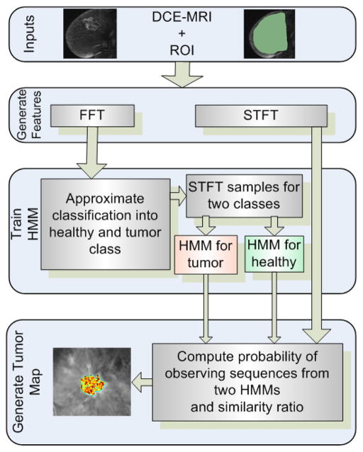
Key techniques used in SLATS include the Fast Fourier transform (FFT), Short-time Fourier Transform (STFT), the k-means clustering algorithm and the Hidden Markov Model (HMM). The flow chart of the algorithm is shown in Figure 1. Our algorithm is based on modeling the transition of each voxel in time and segmenting the voxel into healthy and tumor classes. First, a region of interest (ROI) is delineated by a human operator on the dynamic image data. The time-intensity profile of each voxel in the ROI is provided to the FFT algorithm, and the frequency components of the time-intensity profiles are computed. The voxels are approximately clustered based on the magnitude of the FFT into “tissue type” classes using the k-means clustering algorithm. A small sample of points from the two classes of voxels are then provided to train two discrete HMMs corresponding to healthy (normal parenchyma) (λ₁) and tumor (λ₂) classes. For the remaining pixels, the probability of observing the discrete sequence is computed from HMM λ₁ and HMM λ₂. A similarity ratio χ is then evaluated to determine the similarity to the healthy or tumor class. The ratio χ is then converted to a color scale and overlaid with the original images to determine the position of the tumor. We now go over each component of the pipeline in more depth.

Fig. 1.

SLATS

Short-time Fourier Transform

The observation sequence to train the discrete HMM is created from the interpolated time intensity curves. First, the time-domain curves are converted into the corresponding Fourier transforms to extract the information from the enhancement curves. The Fourier transform preserves the information in the signals and can be computed efficiently. However, the Fourier transforms lack the temporal localization of the frequencies. Therefore, we use the Short-Time Fourier Transform (STFT) in short time periods and obtain a feature vector corresponding to each time window [15]. The STFT is computed as,

$${\mathit{STFT}}_x^{\gamma }={\int }_{\tau }[x(\tau )\gamma (\tau -t^{\prime })]e^{-j2\pi \tau }d\tau$$ (1)

where γ(τ − t′) is the sampling window of the trajectory. The Fourier transform in each sampling window is computed by the Fast Fourier Transform (FFT) algorithm. Information loss is minimized by overlapping the STFT windows. In each sampling window, the STFT consists of the magnitude of N discrete frequency contributions. Multiplication of the signal by the relatively short window effectively suppresses the signal outside the analysis time point, thereby acting as a bandpass filter.

Vector Quantization

Since the HMM structure considered in this paper is discrete, we convert the N tuple vector in each time interval into a single discrete observation symbol using the k-means clustering algorithm [16]. The k-means algorithm partitions the p vectors at different time intervals into L = 16 sets so as to minimize the within-cluster sum of squares. The discrete observation symbol is the index of the codebook vector closest to the given N tuple vector, i.e., the cluster in which the vector belongs.

Hidden Markov Model

Our HMM analysis is based on the approach and notation of Rabiner [17]. The parameters of the HMM model are defined as follows:

• The HMM is assumed to have N (= 4) states. The transition probability between state i to j is given by

  $$a_{ij}=P(q_{t+1}=S_j\mid q_t=S_i)\text{and}A=\{a_{ij}\}$$ (2)
• Each state also has M (= 16) possible observation symbols O_t. The probability of observing a particular symbol O_t in state j is

  $$b_j=P(O_t\mid q_t=S_j)\text{and}B=\{b_j\}$$ (3)

• Also a state prior π_i is defined, which is initial probability of beginning in S_i

In short the HMM can be represented as λ = (A,B, π). The model λ is trained according to the time-intensity curves obtained from a sample of points from each class.

HMM Training

Having generated the discrete observation symbols, the observation sequence is provided to the HMM network to obtain the updated model λ̂. The parameters of the models are estimated by maximizing the auxiliary function

$$Q(\lambda ,\overline{\lambda })=\sum _{Q}P(Q\mid O,\lambda )log[P(O,Q\mid \overline{\lambda })]$$ (4)

This optimization problem is solved iteratively by the Baum-Welch method [17]. Two HMMs are trained correspoding to the “Healthy” (λ₁) and “Tumor” (λ₂) class.

HMM Prediction

Once the HMMs have been trained, the next step is to measure whether the HMM classifies the nature of the time-intensity curves. That is, we evaluate the likelihood that a particular HMM describes the observation sequence. The probability of predicting the observation sequence given the HMM model is computed inductively using the forward-backward algorithm:

$$P(O\mid \lambda )=\sum _{i=1}^N{\alpha }_T(i)$$ (5)

where α_T (i) = P(O₁O₂…O_T, q_t = S_i|λ) is the forward variable. The reader is referred to [17] for greater details.

Similarity Ratio

A similarity ratio χ_j is computed to evaluate if a particular point j belongs to the tumor or healthy class and is converted to a scalar color map. The measure is defined as

$${\chi }_j=log(P(O_j\mid {\lambda }_1))/log(P(O_j\mid {\lambda }_2))$$ (6)

III. Results

Ten breast examinations of women diagnosed with node negative and estrogen receptor positive breast cancer were analyzed under a protocol approved by the Institutional Review Board and compliant with Health Insurance Portability and Accountability Act (HIPAA). The average age of the patients was 55 years. The women were imaged prone in a 1.5T scanner (GE LX echo, GE Healthcare, or Siemens Sonata, Siemens); matrix size: 512 × 512; slice thickness: 2.4–4.4 mm; flip angle: 25° or 30°. The DCE-MRI consisted of 4 data points. For each breast examination, an expert radiologist delineated the primary node of the tumor using the DCE-MRI run in a movie format. A visual inspection of brightly enhanced portions of the DCE-MRI was utilized for delineating the tumor boundaries. The radiologist focused on delineating only the dominant mass-like portion of the malignancy and not on any associated non-mass like or smaller components, for the purposes of a study focusing on mass characterization by DCE-MRI. This segmentation was considered as the reference for SLATS. Although, this segmentation mask cannot be considered as a gold standard, this provides a good reference for SLATS to verify if the algorithm can perform as good or better than a radiologist.

The 4D images were loaded in 3D Slicer, an open-source image processing and navigation software (www.slicer.org). A region of interest was delineated on the DCE-MRI using the expert radiologist’s segmentation as a reference. The time-intensity curve for each voxel was logged and provided to SLATS, which was run on MATLAB. The workflow of a typical case is shown in Figure 2.

Fig. 2.

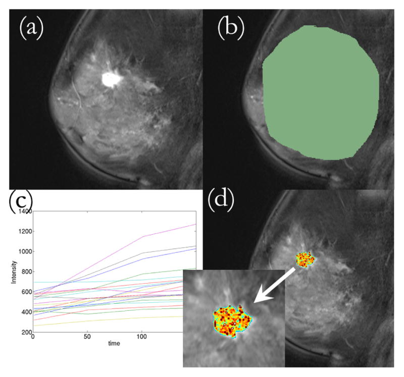
Workflow of the SLATS algorithm. (a) DCE-MRI loaded into 3D Slicer (b) ROI delineated (c) Time-intensity curves obtained from all voxels under ROI and provided to SLATS (d) Tumor map is generated

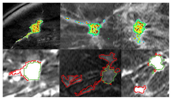
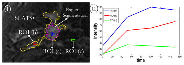
The result for SLATS compared to the radiologist’s finding is shown in Figure 3. All the tumor foci delineated by the expert radiologist were detected by SLATS resulting in a sensitivity of 100%. For three cases an additional focus of tumor was also detected, resulting in an accuracy of 77%. As mentioned earlier, the radiologist only focussed on the dominant tumor mass, for the purposes of a study focusing on mass characterization by DCE-MRI. This additional focus could either be spurious noise detected by SLATS or could be a true positive. In the absence of biopsy results, the only way to characterize the additional mass is by observing the type of enhancement in the additional mass and compare the enhancement to the time-intensity curves in the primary mass and a known normal parenchyma region. Figure 4(ii) shows the time-intensity curve at three locations shown in Figure 4(i). As seen in Figure 4(i), ROI (a) corresponds to the primary mass, ROI (b) to the secondary mass and ROI (c) to normal parenchyma tissue. Figure 4(ii) shows that the enhancement curve for ROI(b) more closely resembles that of ROI(a) than ROI(c), thereby implying that the secondary mass is more likely to correspond to tumor than normal parenchyma tissue. This was also independently confirmed in a blinded study conducted by a second radiologist.

Fig. 3.

Results of SLATS for 6 cases. (Top row) SLATS tumor map with segmentation outline by an expert radiologist shown in green (Bottom row) Overlap between SLATS and expert segmentation shown in green. Excess region segmented by SLATS shown in red.

Fig. 4.

(i) DCE-MRI with SLATS and expert segmentation showing three ROI. ROI(a): within the mass detected by SLATS and Experts, ROI(b): within the mass detected by SLATS only, ROI(c): outside SLATS and Expert segmentation region (ii) Time-intensity curves corresponding to the three ROIs

The Dice Similarity Coefficient (DSC), which measures the amount of overlap between SLATS detected tumor and manually outlined tumor, is 0.72 ± 0.2. Considering only the primary mass, the DSC is measured to be 0.81 ± 0.08, thereby showing a good correlation between the SLATS detected tumor region and the manually segmented region. In order to test the stability of the algorithm, the DCE-MRI and the associated tumor map T_t was translated by an arbitrary amount, which in this case was RAS (−20, 37, 16) mm. The ROI was chosen again and the time-intensity profiles were logged and provided to the SLATS algorithm based on which the tumor map T was obtained. The DSC computed between T_t and T was 0.99, thereby showing a robust stability to translational disturbances. In addition, random noise was also added to the DCE-MRI to evaluate the noise disturbance rejection capability. The DSC between the tumor map generated from the noisy DCE-MRI and original map was 0.995, showing excellent noise rejection capability. The SLATS result was also compared to the tumor maps generated from CADstream, a commercially available software from GE Healthcare Systems, for three patients. The DSC computed between the SLATS and CADstream generated tumor map is 0.85. The result, shown for two patient cases in Figure 5, illustrates differences in the tumor maps generated from SLATS and CADstream. A detailed validation in a larger study is required to confirm the differences in the two tumor maps.

Fig. 5.

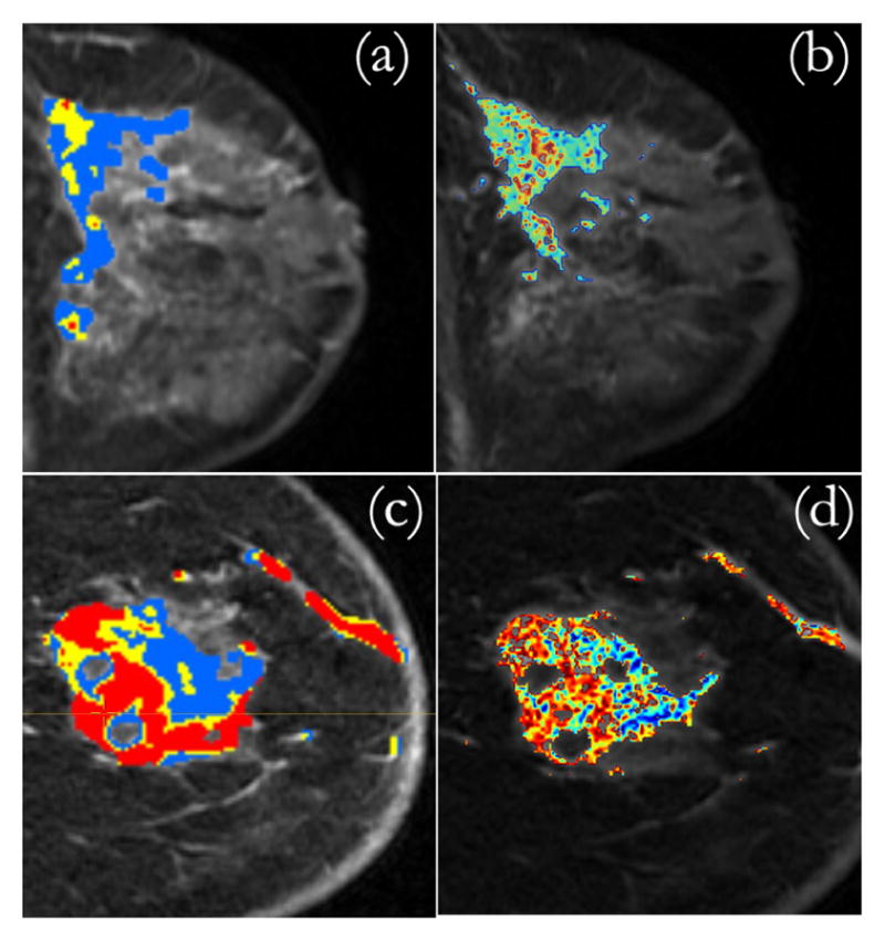
(a) CADstream map (b) SLATS tumor map generated for Patient 1. (c) CADstream map (d) SLATS tumor map generated for Patient 2.

IV. Conclusion

In this paper, we describe a novel algorithm to segment regions of tumor. SLATS uses the frequency components of the time-intensity curves, thereby making the algorithm invariant to absolute intensities, MR bias or choice of pulse sequence. The algorithm is robust to noise and translational disturbances. However, deformation of the breast during imaging needs to be addressed using non-linear deformable registration algorithms. SLATS shows very high sensitivity and accuracy when compared to an expert radiologist’s finding. Further validation of the algorithm using biopsy samples obtained under image-guidance is currently underway.

References

- 1.Eliat P-A, et al. Magnetic resonance imaging contrast-enhanced relaxometry of breast tumors: an MRI multicenter investigation concerning 100 patients. Magnetic Resonance Imaging. 2004;22(4):475– 481. doi: 10.1016/j.mri.2004.01.024. [DOI] [PubMed] [Google Scholar]
- 2.Radjenovic A, Dall BJ, Ridgway JP, Smith MA. Measurement of pharmacokinetic parameters in histologically graded invasive breast tumours using dynamic contrast-enhanced MRI. Br J Radiol. 2008;81(962):120–128. doi: 10.1259/bjr/98435332. [DOI] [PubMed] [Google Scholar]
- 3.Pickles MD, Manton DJ, Lowry M, Turnbull LW. Prognostic value of pre-treatment DCE-MRI parameters in predicting disease free and overall survival for breast cancer patients undergoing neoadjuvant chemotherapy. European Journal of Radiology. 2009;71(3):498– 505. doi: 10.1016/j.ejrad.2008.05.007. [DOI] [PubMed] [Google Scholar]
- 4.Tuncbilek N, Tokatli F, Altaner S, Sezer A, Tre M, Omurlu IK, Temizoz O. Prognostic value DCE-MRI parameters in predicting factor disease free survival and overall survival for breast cancer patients. European Journal of Radiology. 2011;71(3):498– 505. doi: 10.1016/j.ejrad.2011.02.021. [DOI] [PubMed] [Google Scholar]
- 5.Bhooshan N, Giger ML, Jansen SA, Li H, Lan L, Newstead GM. Cancerous breast lesions on dynamic contrast-enhanced MR images: Computerized characterization for image-based prognostic markers. Radiology. 2010;254(3):680–690. doi: 10.1148/radiol.09090838. [DOI] [PMC free article] [PubMed] [Google Scholar]
- 6.Hylton N. Dynamic contrast-enhanced magnetic resonance imaging as an imaging biomarker. Journal of Clinical Oncology. 2006;24(20):3293–3298. doi: 10.1200/JCO.2006.06.8080. [DOI] [PubMed] [Google Scholar]
- 7.El Khouli Riham H, Macura Katarzyna J, Jacobs Michael A, Khalil Tarek H, Kamel Ihab R, Dwyer Andrew, Bluemke David A. Dynamic contrast-enhanced MRI of the breast: Quantitative method for kinetic curve type assessment. American Journal of Roentgenology. 2009;193(4):W295–W300. doi: 10.2214/AJR.09.2483. [DOI] [PMC free article] [PubMed] [Google Scholar]
- 8.Leach MO, et al. The assessment of antiangiogenic and antivascular therapies in early-stage clinical trials using magnetic resonance imaging: issues and recommendations. British Journal of Cancer. 2005;92:15991610. doi: 10.1038/sj.bjc.6602550. [DOI] [PMC free article] [PubMed] [Google Scholar]
- 9.Kety SS. The theory and applications of the exchange of inert gas at the lungs and tissues. Pharmacological Reviews. 1951;3(1):1–41. [PubMed] [Google Scholar]
- 10.Tofts PS, Kermode AG. Measurement of the blood-brain barrier permeability and leakage space using dynamic MR imaging. 1. fundamental concepts. Magnetic Resonance in Medicine. 1991;17(2):357–367. doi: 10.1002/mrm.1910170208. [DOI] [PubMed] [Google Scholar]
- 11.St Lawrence KS, Lee T-Y. An adiabatic approximation to the tissue homogeneity model for water exchange in the brain: I. theoretical derivation. Journal of Cerebral Blood Flow & Metabolism. 1998;18:1365–1377. doi: 10.1097/00004647-199812000-00011. [DOI] [PubMed] [Google Scholar]
- 12.Sourbron SP, Buckley DL. On the scope and interpretation of the tofts models for DCE-MRI. Magnetic Resonance in Medicine. 2011;66(3):735–745. doi: 10.1002/mrm.22861. [DOI] [PubMed] [Google Scholar]
- 13.Chen W, Giger ML, Bick U. A Fuzzy C-Means (FCM)-based approach for computerized segmentation of breast lesions in dynamic contrast-enhanced MR images. Academic Radiology. 2006;13(1):63– 72. doi: 10.1016/j.acra.2005.08.035. [DOI] [PubMed] [Google Scholar]
- 14.Shafer CM, Seewaldt VL, Lo JY. Validation of a 3D Hidden-Markov model for breast tissue segmentation and density estimation from MR and tomosynthesis images. Biomedical Sciences and Engineering Conference (BSEC) 2011:1–4. [Google Scholar]
- 15.Hlawatsch F, Bordeaux-Bartles D. Linear and quadratic time-frequency signal representation. IEEE Signal Process. 1992;9:21–67. [Google Scholar]
- 16.Likas A, Vlassisb N, Verbeekb JJ. The global k-means clustering algorithm. Pattern Recognition. 2003;36:451–461. [Google Scholar]
- 17.Rabiner LR. A tutorial on Hidden Markov models and selected applications in speech recognition. Proceeding of the IEEE. 1989;77:257–286. [Google Scholar]