Spatiotemporal trends in teen birth rates in the USA, 2003–2012

Summary

The objective of this analysis was to explore temporal and spatial variation in teen birth rates TBRs across counties in the USA, from 2003 to 2012, by using hierarchical Bayesian models. Prior examination of spatiotemporal variation in TBRs has been limited by the reliance on large-scale geographies such as states, because of the potential instability in TBRs at smaller geographical scales such as counties. We implemented hierarchical Bayesian models with space–time interaction terms and spatially structured and unstructured random effects to produce smoothed county level TBR estimates, allowing for examination of spatiotemporal patterns and trends in TBRs at a smaller geographic scale across the USA. The results may help to highlight US counties where TBRs are higher or lower and to inform efforts to reduce birth rates to adolescents in the USA further.

1. Introduction

Teen birth rates (TBRs) have declined over the past several years across nearly every state in the USA (Hamilton and Ventura, 2012). In 2013, there were 26.5 births for every 1000 adolescent females (15–19 years of age), representing a decline of 57% from TBRs in 1991 (Martin et al., 2015). The 1991 TBR, 61.8 births per 1000 women aged 15–19 years, marks both a recent high and the start of the nearly continuous downward trend.

TBRs vary by state, with higher values seen across the south and south-western regions of the country and lower TBRs observed in the north-east (Ventura et al., 2014). Moreover, the declines in TBRs evidenced over the past several years have varied by state, with steeper declines in the Southeast, Mountain, Pacific and upper Midwest areas of the USA (Ventura et al., 2014). However, county level variation in TBRs and corresponding trends over time have not been explored. County level analyses have largely not been undertaken because of the potential instability of the direct estimates at this level, which is a greater problem for counties that are sparsely populated. Direct estimates for TBRs are typically suppressed in counties with fewer than 20 births because of concerns about the stability and reliability of the estimates. To address these problems, we employed hierarchical Bayesian models with space–time interaction terms as well as spatially structured and unstructured random effects to produce stable county level estimates of TBRs from 2003 to 2012.

Past studies have looked at the risk factors affecting teen pregnancies (Chang et al., 1998; Dennison, 2004; Kirby, 2005; National Latino Research Center, 2005a,b; Kearney and Levine, 2012; Kuang and Williams, 2013; National Campaign to Prevent Teen and Unplanned Pregnancy, 2013) and reported that poverty, lower levels of education, unemployment and smoking, drug and alcohol abuse issues are associated with elevated TBRs. Generally, reduced socio-economic opportunity has been associated with higher TBRs (Kost et al., 2010; Kearney and Levine, 2011, 2012; Kost and Henshaw, 2012; Penman-Aguilar et al., 2013; Population Reference Bureau, 2012; Shoff and Yang, 2012). However, most prior studies have focused on TBRs at the national level or state level. It is important to note that these factors also vary within states and over time.

The objective of this analysis was to explore temporal and spatial variation in TBRs across 3138 counties in the USA, from 2003 to 2012. Bayesian hierarchical space–time interaction models (Besag et al., 1991; Besag and Kooperberg, 1995; Knorr-Held and Besag, 1998; Lagazio et al., 2001) were used to predict TBRs at the county level. These county level TBR estimates were mapped to examine geographic and temporal variation in TBRs across the USA. Results may help to highlight US counties where TBRs are significantly higher or lower than a selected target.

The plan of this paper is as follows. Section 2 contains information on data and methods. In Section 3, we discuss methods for evaluating model fit, comparisons of the models proposed and residual analysis. Sections 4 and 5 discuss results and findings. Finally, in Section 6, we discuss conclusions and future research directions.

The programs that were used to analyse the data can be obtained from http://wileyonlinelibrary.com/journal/rss-datasets

2. Methods

2.1. Description of data and sources

Data on the number of live births for women aged 15–19 years were extracted from the national vital statistics birth data files for the years 2003–2012 (e.g. National Center for Health Statistics (2012)). These data were then aggregated to the county level to provide a teen birth count for each county per year. The denominators to calculate TBRs were obtained from intercensal and post-censal population estimates of the number of females aged 15–19 years residing within each county over the same time period. These population denominators were extracted from the files containing intercensal and post-censal bridged race population estimates provided by the National Center for Health Statistics. For each year, the July population estimates were used with the exception of the year of the decennial census, 2010, for which the April estimates were used. Using these two sources of data, annual TBRs were calculated at the county level.

During the decade of interest, county borders in Alaska changed such that new counties were formed and others were merged. These changes were reflected in the population files but not in the natality files. For this reason, two counties in Alaska had to be collapsed so that the birth and population counts were comparable. Additionally, Kalawao County, which is a remote island county in Hawaii, recorded no births and the census estimates indicated a denominator of 0 (i.e. zero females between the ages of 15 and 19 years residing in the county from 2003 to 2012). Hence, Kalawao County was removed from the analysis and the final analysis was conducted on 3138 counties in the USA.

County level covariates including various socio-economic indicators (e.g. per capita income, percentage of the county in poverty and the unemployment rate) and demographic variables (e.g. racial composition, proportion of foreign-born residents and level of education) were obtained from the area resource file (Health Resources and Services Administration, 2012). These variables were included in a principal component analysis that is described later in Section 4.1. In addition to these covariates, the number of family planning and Title X clinics by county, based on data provided by the Guttmacher Institute (2010), were initially included in the models but subsequently removed because of the lack of statistical association with TBRs at the county level.

The broad scale trends in TBRs were examined by census regions (Midwest, Northeast, South, and West), census divisions (East North Central, East South, Mid-Atlantic, Mountain, New England, Pacific, South Atlantic, West North Central and West South Central) and urban–rural designations as classified by the National Center for Health Statistics (https://www.census.gov/geo/reference/gtc_census_divreg.html) (Ingram, 2012). Census divisions are groupings of states and the District of Columbia that are subdivisions of the four census regions. The urban–rural classification scheme identifies large central counties with 1 million or more residents that contain an entire population of the largest principal city or are completely contained within the largest principal city, or contain at least 250 000 residents of a principal city of the metropolitan statistical area. Counties in metropolitan statistical areas of 1 million or more residents that do not meet criteria for being large central (e.g. suburbs) qualify as large fringe. Medium metro are counties with a population between 250 000 and 999 999 and small metro counties have a population less than 250 000. Micropolitan counties are those consisting of an urban cluster of 10 000 to fewer than 50 000 residents. Counties outside core-based statistical areas are classified as non-core or rural.

For a list of the variables that were used in the final analysis refer to Table 1.

Table 1.

Variables included in the principal component analysis

Variable	Principal component analysis component
	1	2	3
% white population 2010	−30	2	89†
% non-Hispanic white population 2010	−25	11	92†
Median household income 2011	−78†	43†	−17
% persons in poverty 2011	89†	−28	−26
% persons in poverty 2010	89†	−29	−26
% persons in poverty 2009	91†	−27	−22
% persons in poverty 2008	91†	−30	−22
% persons in poverty 2007	90†	−29	−24
% persons in poverty 2006	89†	−30	−25
% persons in poverty 2005	89†	−29	−26
% persons in poverty 2000	84†	−35	−27
% persons age 0–17 years in poverty 2011	84†	−37	−20
% persons below poverty level 2006–2010	87†	−27	−25
% families below poverty level 2006–2010	81†	−35	−29
% persons age ≥ 25 years with less than High School Diploma 2006–2010	42†	−82†	−30
% persons age ≥ 25 years with High School Diploma or more 2006–2010	−42†	82†	30
% persons age ≥ 25 years with ≥ 4 years college 2006–2010	−32	81†	−23
Unemployment rate, ≥ 16 years, 2005	52†	−29	−21

^†Significant positive (or negative) contribution to the component score.

2.2. Models

We fit a hierarchical Bayesian model by using methods similar to those established by Xia (1997), Wall (2004) and Lawson (2013) (chapter 12) for epidemiological studies and disease mapping. Let y_it be the counts of teen births in county i and year t, and n_it the counts of teen population in county i and year t. Then, y_it ~ binomial(n_it, p_it ), i = 1, . . . , m counties and t = 1, . . . , T years, where p_it is the probability of teen births in county i at time t.

The general space–time model structure for modelling p_it that was laid down by Böhning et al. (2000), Lagazio et al. (2001), Lawson (2013) (chapter 12), Knorr-Held and Besag (1998) and Rao and Yu (1994) is

$$\text{logit}(p_{it})={\alpha }_0+A_i+B_t+C_{it},$$

where A_i is the spatial group, B_t is the temporal group and C_it is the space–time interaction group.

Several models were implemented following this general space–time modelling framework. The two best competing models are presented here, representing two special cases of the general space–time model. One case follows the approach of Besag et al. (1991) and employs spatially structured random effects to account for spatial auto-correlation in TBRs; this model is referred to as the convolution model. The alternative approach also employs random effects following the approach of Carlin and Louis (2009), but these terms are not spatially structured in nature. These two alternative model specifications are described below.

2.2.1. Besag–York–Mollié model

The raw county level TBRs exhibited strong spatial auto-correlation as indicated by a Moran’s I -test for spatial auto-correlation. Some of the spatial auto-correlation can be modelled by including spatially patterned covariates, but residual spatial auto-correlation often remains due to unmeasured confounders, aggregation effects or neighbouring effects (Lawson (2013) (chapter 5) and Lee (2013)). Thus, a priori, we expected that models accounting for such autocorrelation might be necessary. A common approach to tackle spatial auto-correlation is to introduce spatially structured random effects into the model. These random effects are specified by conditional auto-regressive priors via the adjacency matrix of the counties (Besag et al., 1991). Hence, we implemented the convolution model (Besag et al., 1991) to account for this potential spatial auto-correlation in TBRs (Besag et al., 1991). The convolution model is

$$\text{logit}(p_{it})={\alpha }_0+a_{1i}\ast {\text{year}}_t+{X_i}^{\prime }\mathit{\gamma }+u_i+v_i+{\psi }_{it}.$$

The convolution model includes

1. a logit link function log{p_it /(1 − p_it )},

2. α₀, an intercept,

3. a time trend term a_1i * year_t,

4. X_i′γ, where X_i is the ith row of the covariates matrix and γ is a vector of regression parameters,

5. spatial random effects u_i by county to model strong spatial auto-correlation, i = 1, . . . , m counties,

6. non-spatial random effects v_i by county to model residual spatial auto-correlations that were not dealt with by our spatial random effects, u_i, i = 1, . . . , m counties, and

7. a space–time interaction term ψ_it , a random effect where ψ_it is a function of its past values, ψ_i,t−1, plus an error term.

Parameters under (e) are modelled via normal conditional auto-regressive priors (Besag et al., 1991). Parameters under (f) are modelled via normal conditional priors. Parameters under (g) are modelled via type II random-walk interactions (Knorr-Held and Rasser, 2000), which are included to account for any residual spatiotemporal dependence or variation that is not captured by the spatial or temporal main effects. The values for a given county in a given year depend on the values that were observed for that county in the previous year plus a residual (Knorr-Held and Rasser (2000) and Lawson (2013) (chapter 12)).

2.2.2. Basic model

To discern whether spatially structured random effects offer major improvements in model fit, a basic model without spatially structured random effects was also examined. The basic model is

$$\text{logit}(p_{it})={\beta }_{1i}+{\beta }_{2i}{\text{year}}_t+{X_i}^{\prime }\mathit{\gamma }+{\psi }_{it}.$$

The basic model includes (Carlin and Louis (2009) (chapter 2))

1. a logit link function log{p_it /(1 − p_it )},

2. β_1i, the intercept,

3. the time trend term β_2i* year_t.

4. X_i′γ, where X_i is the ith row of the covariates matrix and γ is a vector of regression parameters, and

5. ψ_it, a random effect where ψ_it is a function of its past values, ψ_i,t−1, plus an error term.

Parameters under (d) and (e) are modelled as in the convolution model that was described above. Specifically, ψ_it is modelled via a type II random-walk interaction (Knorr-Held and Rasser, 2000). Additionally, the random intercept (b) can be thought of as the combination of two terms from the convolution model, α₀ + v_i. Thus, the basic model differs from the convolution model in that the basic model does not include the spatially structured random-effect term that appears in the convolution model.

Several other models were implemented in WinBUGS, including simpler versions of the two models that were described above. Because of poor convergence or fit of these other models, we present results for only the two best performing models (see Section 4.2).

2.2.3. Prior distribution assumptions

Since the conditional auto-regressive normal prior is assigned for the spatial random effects u_i in the Besag–York–Mollié (BYM) model, with sum-to-zero constraints on the spatial random-effect term (Lunn et al., 2013), a flat prior is assumed on the intercept α₀. For the basic model, the county-specific intercepts β_1i and time trend terms β_2i are modelled to arise from a multivariate normal prior distribution with mean μ and a precision matrix ϒ which is assigned a Wishart (R,2) prior distribution, where R is set to be a diagonal matrix (Carlin and Louis, 2009) (chapter 2)). Specifically,

1. β_i = (β_1i, β_2i)′ and

2. β_i ~ ^IIDN(μ, ϒ).

The hyperprior of μ is chosen to be very vague by choosing the precision matrix to be very small. The hyperprior of ϒ is also made vague by setting the degrees of freedom equal to 2, the lowest for which the Wishart prior is proper, and using an approximate value for the precision matrix (Carlin and Louis, 2009).

Sensitivity analyses were conducted with different prior values on the precisions with a choice of parameters leading to priors with most of the probability mass around the expected values of the variance parameters (Griffin and Brown, 2010; Furrer and Sain, 2010). The choice of inverse gamma priors IG(0.01, 0.01) (Gelman, 2006) resulted in the lowest deviance information criterion (DIC) in model comparisons (the DIC is described in detail in Section 3.4), though the posterior estimates were unaffected by the choice of the priors. The time trend term a_1i in the basic model, the non-spatial random effects v_i in the BYM model and the fixed effects γ_i in both the BYM and the basic model are assumed to be independent zero-mean Gaussian distributions with inverse gamma priors IG(0.01, 0.01) on the precisions for all the components. The precisions on the spatial random effects u_i in the BYM model and the random effect ψ_it in both the BYM and the basic model are also assigned inverse gamma priors IG(0.01, 0.01). More detailed information on the statistical formulation of models and priors can be seen in Appendix A.

2.3. Markov chain Monte Carlo sampling

Analyses were implemented via Markov chain Monte Carlo (MCMC) simulations using the WinBUGS freeware (Lawson, 2013; Ntzoufras, 2009; Spiegelhalter et al., 2003) in the software R (Ntzoufras, 2009) via the library R2WinBUGS. We used the Brooks–Gelman–Rubin diagnostic tool, density, auto-correlation and history plots to confirm convergence, keeping every 40th value after a burn-in period of 50 000 for 100 000 iterations. We based inference on an additional 100 000 iterations after convergence. In the converged sample we compared the models by using the DIC (Spiegelhalter et al., 2002), Bayesian p-values and Gelfand and Ghosh (1998) statistics. Maps were produced by using R and the geographical information system ArcGIS (Environmental Systems Research Institute, 2011).

2.4. Exceedance probabilities

The posterior probabilities p_it that were derived from the best model were used to detect areas with elevated TBRs (Lawson, 2013). The exceedance probability is defined as the probability that the posterior probability p_it exceeds some threshold c. If the posterior sampled values are $p_{it}^1,\dots ,p_{it}^n$, where n is the number of samples, the exceedance probability can be calculated as

$$\widehat{Pr}(p_{it}>c)=\sum _{i=1}^{n}I(p_{it}^i>c)/n$$ (1)

where I(a) is an indicator function.

The raw county level TBRs ranged from 0 to 133 per 1000 in 2012, with a mean of 36 per 1000 (median, 34 per 1000; interquartile range, 21–48 per 1000). By contrast, in 2003, the raw county level TBRs ranged from 0 to 147 per 1000 with a mean of 44 per 1000 (median, 42 per 1000; interquartile range, 28–58 per 1000). The threshold for the exceedance probability c was therefore chosen to reflect a TBR of 36 per 1000, which coincides with the mean raw TBR across all included counties for the year 2012. These exceedance probabilities were mapped, grouping counties into those with high likelihood of exceeding the threshold and counties with low likelihood of exceeding the threshold.

3. Model check and selection

3.1. Model check: Bayesian p-value

The structural assumptions of the fitted model can be ascertained by the use of posterior predictive model checks (Ntzoufras, 2009; Gelman et al., 1995). The evaluation of the posterior distribution of the Bayesian model is done by comparing the observed data y^obs with the posterior predictive distribution or replicates y^rep. We generated replicate data sets y^rep for each posterior draw of the model parameters and then calculated a test quantity T(y_it, θ) (where θ is the vector of unknown parameters) representing an omnibus goodness-of-fit measure, defined as

$$T(y_{it},\theta )=\sum _{i,t}\frac{{\{y_{it}-E(y_{it}\mid \theta )\}}^2}{\text{variance}(y_{it}\mid \theta )}$$ (2)

(Gelman et al. (1995) (page 172)), where the summation is over all sampled observations. Bayesian p-values associated with the test quantity were computed; values close to 0 or 1 (Gelman et al., 1995) suggest that the model might not be a good fit.

3.2. Model check: comparison with direct estimates of state teen birth rates

The posterior probabilities that are produced by each model for each county and year were summed by state and weighted by county population size as a proportion of state population size to create state model-based estimates of the TBR for each year. These model-based estimates were compared with the direct estimates of the TBR for each state and year to ascertain whether one of the models performed better or worse than another in terms of matching the state direct estimates.

3.3. Model selection: Gelfand and Ghosh statistic

Models were also evaluated by using the Gelfand and Ghosh statistic, which compares observed data y^obs with the replicates y^rep. This approach minimizes the posterior predictive loss over all possible predictions of future observations y^rep (Ando, 2010; Gelfand and Ghosh, 1998). The replicated data set is used to compute the posterior predictive mean and variance for each observation. A goodness-of-fit measure G, which is the error sum of squares of the difference between the data and its posterior predictive mean, is computed. It is calculated as

$$G=\sum _{i,t}{\{y_{it}-E(y_{it}\mid \theta )\}}^2$$ (3)

(where θ is the vector of unknown parameters). We calculate P, which is the sum over all observations of the posterior predictive variances. It is defined as

$$P=\sum _{i,t}\text{variance}(y_{it}\mid \theta ).$$ (4)

With the increasing complexity in models, G will decrease but P will begin to increase (Gelfand and Ghosh, 1998). The statistic D is calculated as G + P, which is a combination of goodness of fit and variability (Barker et al., 2013). Models with smaller D-values are selected.

3.4. Deviance information criterion for model comparison

Models can be compared by using a criterion utilizing a trade-off between the fit of the data and the corresponding complexity of the model. The DIC was proposed by Spiegelhalter et al. (2002) and is widely used in Bayesian modelling for comparing hierarchical models (Lawson, 2013; Ntzoufras, 2009; Spiegelhalter et al., 2002, 2003). A model fit can be summarized with deviance. We define deviance as

$$D(\theta )=-2log\{L(y_{it}\mid \theta )\},$$ (5)

where y_it are the data, θ is the vector of unknown parameters of the model and L(y_it |θ) is the likelihood function. But deviance does not take into account the complexity of the model. A way to estimate the complexity is by measuring the effective number of parameters in a model (Spiegelhalter et al., 2002), pD, defined as

$$\text{pD}=E_{\theta \mid y}(D)-D\{E_{\theta \mid y}(D)\}=\overline{D}-D(\overline{\theta }),$$ (6)

where D̄ = E_θ|y (D) is the posterior mean deviance and D(θ̄) = D{E_θ|y (D)} is the deviance evaluated at the posterior mean of the parameters. The DIC is then defined as

$$\text{DIC}=D(\overline{\theta })+2p_D=\overline{D}+p_D.$$ (7)

Models with smaller DIC are preferred.

3.5. Residual analysis

We employed further model checks by analysing the residuals from each model. Residuals were defined as the difference between the model-based and direct estimates of the TBR for each county and year. The distribution of the residuals was inspected for deviations from normality. Residuals were also examined in relation to county size and year to determine whether there were potential non-linear patterns in TBRs that were not accounted for by the model.

4. Results

4.1. Principal component analysis

Including covariates can enhance small area predictions. On the basis of the past research on risk factors affecting teen pregnancies at the state and national level (Chang et al., 1998; Dennison, 2004; Kearney and Levine, 2011, 2012; Kuang and Williams, 2013; Penman-Aguilar et al., 2013; Population Reference Bureau, 2012) 91 county level covariates were initially considered as potential predictors and, of these, 18 had an absolute Spearman rank correlation greater than 0.4 with the TBRs for the majority of the years. County level covariates included various socio-economic indicators (e.g. per capita income, percentage of the county in poverty and the unemployment rate) and demographic variables (e.g. racial composition, proportion of foreign-born residents and education level), measured at different time points, and were obtained from area resource files (Health Resources and Services Administration, 2012). The aggregated covariates were also examined in addition to the individual year covariates. Collinearity within this reduced set of predictors was suspected and thus, to reduce and transform data in the presence of multicollinearity, a principal component analysis was conducted. A probabilistic version of principal component analysis (Tipping and Bishop, 1999) was also investigated. Both of the approaches provided nearly identical results. Hence, the orthogonal component scores derived from the simpler principal component analysis were included.

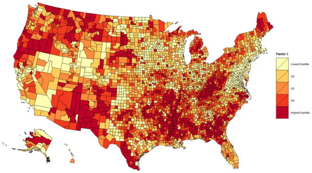
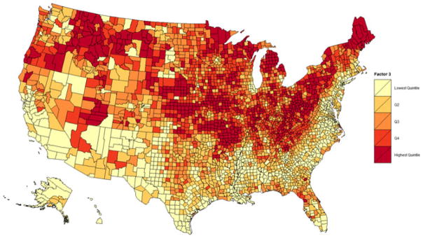
The principal component analysis, using a varimax rotation, indicated that three components were sufficient as they accounted for 88% of the total variation. The variables loading on each of the three components are described in Table 1; the three components largely reflected county level income and poverty, education and percentage non-Hispanic white. The three principal components exhibited substantial geographic variation; these patterns can be seen in the figures. The first factor, corresponding to high levels of poverty and low income (Fig. 1), was highest in the South, Appalachia, New Mexico and parts of the North West and Alaska. The second factor, which is related to higher levels of education (Fig. 2), was highest in the North East and North Central USA, and lowest in the South and west part of Texas. The third factor, percentage white (Fig. 3), was highest in the northern half of the USA, suggesting that the South, the East Coast, South West, Alaska and Hawaii have larger racial or ethnic minority populations.

Fig. 1.

Principal component analysis: construct 1—high poverty and low income (higher TBRs occur in areas where poverty is high and income is low (darker areas))

Fig. 2.

Principal component analysis: construct 2—educational level (higher TBRs occur in low education areas (lighter areas))

Fig. 3.

Principal component analysis: construct 3—race or ethnicity, percentage white (higher TBRs occur in areas where the percentage of the population is predominantly non-white (lighter areas))

4.2. Estimates

Several models were implemented in WinBUGS. The best competing convolution and basic models are described in this analysis. These models were selected on the basis of the DIC, Gelfand and Ghosh statistic and the Bayesian p-values (Table 2). Additionally, convergence was monitored via auto-correlation plots, density plots and history or trace plots. Gelman–Rubin diagnostic plots were also monitored for convergence. Although models without covariates were explored, when the orthogonal component scores were not included, the variance parameters had lumpy history plots or trace plots and high degrees of auto-correlation. After adding the orthogonal component scores, the residual variance distributions were cleaner and the density plots were more normally distributed and had substantially less auto-correlation, suggesting that the inclusion of the orthogonal component scores facilitated model convergence for the random effects, perhaps by accounting for some of the spatial dependence. The Gelman–Rubin diagnostic tool also indicated convergence. Thus, despite not contributing to a major reduction in the DIC, the inclusion of the three orthogonal component scores aided model convergence. Moreover, the MCMC output in Table 3 shows that all the three scores are significantly associated with TBRs (the 95% Bayesian credible intervals exclude 0). The three principal component scores, exceedance probabilities by county and year, and the posterior estimates of the TBRs by county and year were mapped.

Table 2.

Model selection and fit based on the Gelfand and Ghosh statistic, Bayesian p-value and DIC

Model	G	P	D	p-value	DIC
Convolution	6271059417	6076027.018	6277135444	0.5717	210493
Basic	6274389428	6135753.038	6280525182	0.5632	210553

Table 3.

Parameter estimates for the convolution model: orthogonal scores coefficients γ and standard deviation sd of ψ

Node	Mean	sd	Monte Carlo error	2.5 percentile	Median	97.5 percentile
γ1	0.2008	0.006403	2.58×10−4	0.1881	0.2009	0.2131
γ2	−0.2815	0.006194	2.84×10−4	−0.2931	−0.2816	−0.269
γ3	−0.1809	0.006711	4.13×10−4	−0.1936	−0.181	−0.1677
sd(ψ)	0.00706	1.98×10−4	8.27×10−6	0.006681	0.007059	0.007457

4.3. Comparison of models

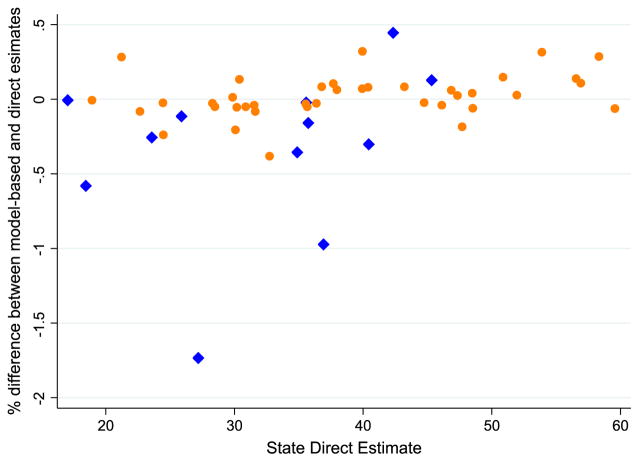
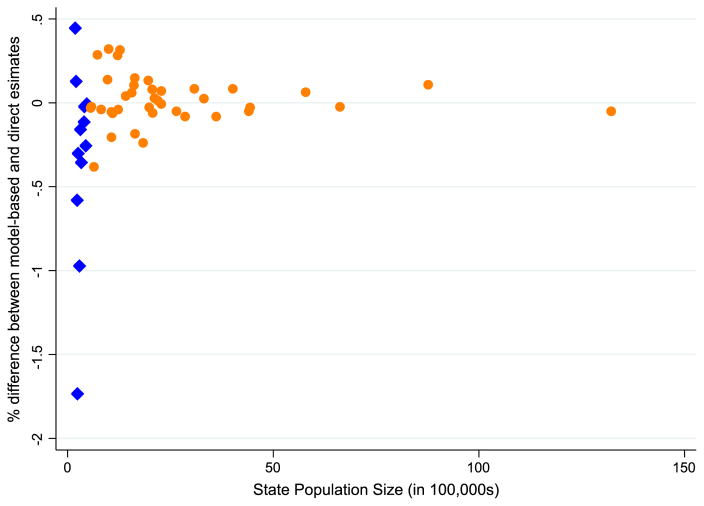
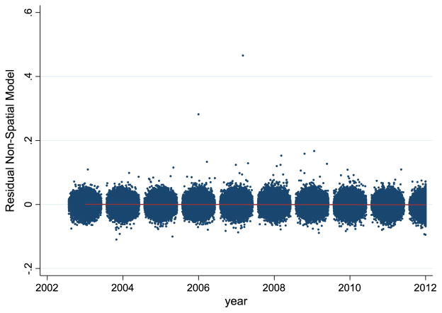
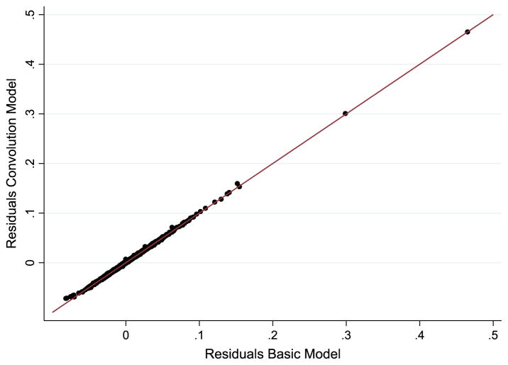
The basic and the BYM models performed similarly in terms of the comparison of model-based and direct estimates of state TBRs. Both models produced state level TBR estimates that were within 1% of the direct estimates for all states except for North Dakota, for which the difference between the model-based and direct estimates was less than 2% (Fig. 4). These differences were larger for states with smaller populations (e.g. North and South Dakota and Wyoming) and smaller for states with larger populations (e.g. Texas, New York, California and Florida) (Fig. 5). At the county level, the residuals did not exhibit any apparent non-linear patterns or major deviations from normality (Fig. 6). Similarly to the comparisons of model-based and direct estimates at the state level, residuals at the county level were generally larger for counties with smaller populations. Both models exhibited similar patterns in the analysis of the residuals; when the residuals from each model were plotted against each other (shown here for the year 2012), they fell along a line of equality (Fig. 7).

Fig. 4.

Differences between state model-based (from the convolution model) and direct estimates: , states with population sizes less than 500000; , states with larger populations

Fig. 5.

Differences between state model-based (from the convolution model) and direct estimates by state population size: , states with population sizes less than 500000; , states with larger populations

Fig. 6.

Residuals from the convolution model by year: the few outlying points reflect counties with very small population denominators, typically n < 20

Fig. 7.

Convolution model and basic model residuals for the year 2012 exhibit similar patterns as they fall on the line of equality

4.4. Model results

The BYM and basic models performed similarly in terms of convergence and residual analysis. In comparisons of model fit, the BYM model provided a better fit with lower DIC and Gelfand and Ghosh statistics (see Table 2). The DIC difference of 10 is considered significant (Spiegelhalter et al., 2002). Hence the convolution model was chosen and is presented below, though it was comparatively computationally intensive. The Bayesian p-values indicated good fit for both the BYM and the basic models.

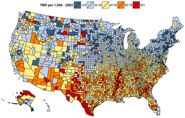
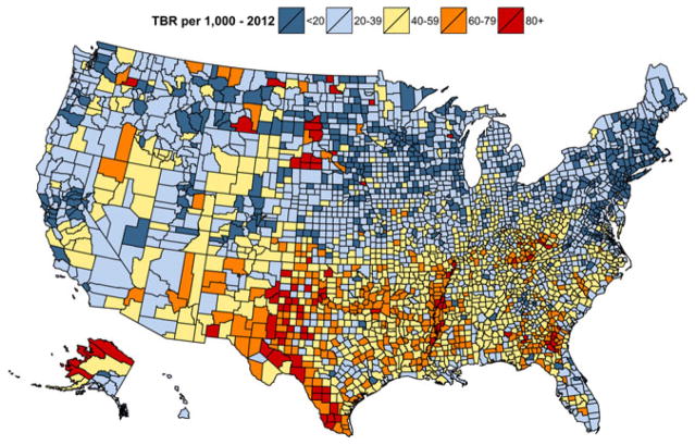
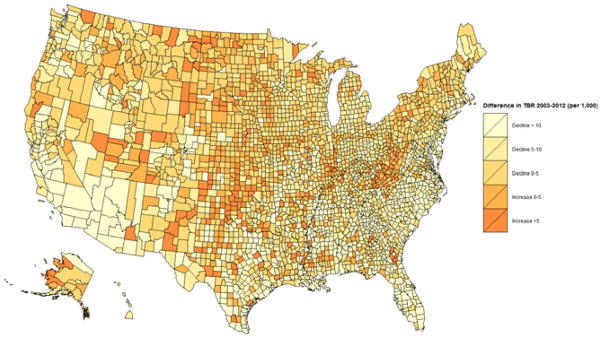
The maps (Figs 8 and 9) show the considerable spatiotemporal variation in county level TBRs from 2003 through to 2012. TBRs ranged from 5.99 to 124.00 in 2003 and 3.56 to 125.70 in 2012, with rates declining in the majority of counties (2489) between those years, increasing in only 648 counties, and essentially unchanged in the remaining county. Among the counties with declining rates, births to teens decreased by 12.52% on average from 2002 to 2012, with declines as great as 79.31% seen. For 413 counties, the TBRs declined from in excess of the exceedance threshold (36 births per 1000) in 2003 to either lower than or not significantly different from the threshold in 2012. In general, birth rates were higher in the southern and south-western regions of the USA (Ventura et al., 2014). However, within those regions and states of high TBR, rates by county show considerable variability among themselves, with rates for several counties across west Texas, along the Mississippi River, as well as parts of Georgia and Alaska, exceeding 80 births per 1000 women aged 15–19 years. Fig. 10 shows the difference in the predicted TBRs (per thousand) for years 2003–2012.

Fig. 8.

Predicted TBRs (per thousand) from the convolution model for year 2003

Fig. 9.

Predicted TBRs (per thousand) from the convolution model for year 2012

Fig. 10.

Difference in predicted TBRs (per thousand) from the convolution model for years 2003–2012

TBRs were highest across the entire study period in the South, and lowest in the Northeast. In 2003, there were bands of particularly higher TBRs (greater than 80 births per 1000 teens) across west Texas and other states in the South along the Mississippi River (e.g. Mississippi, Tennessee and Arkansas), as well as pockets in Alaska, Florida, Georgia, South Carolina, New Mexico and Oklahoma (see Fig. 8). The lowest TBRs in 2003 were in New England (e.g. New Hampshire, Vermont, Massachusetts, Rhode Island and New York), Minnesota, Wisconsin, Illinois and Iowa. In 2012, the geographic patterns were largely similar in terms of areas with the highest and lowest TBRs, but there were fewer counties with TBRs in excess of 80 births per 1000 adolescent females (see Fig. 9). Areas of elevated TBRs remained in parts of Alaska, west Texas, Oklahoma, along the Mississippi River and Georgia.

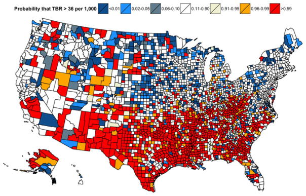
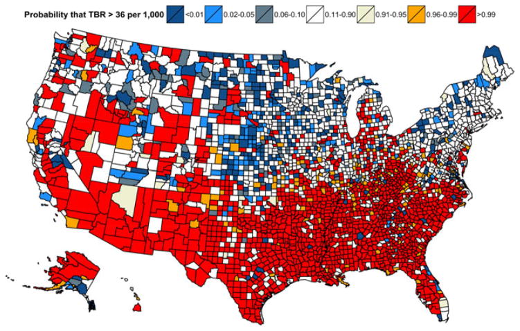
In 2012, most of the counties across the southern states had very high probabilities (p > 0.95) of exceeding the threshold of 36 per 1000 (Fig. 11). In contrast, most of the counties in New England and the states around the Great Lakes had very low probabilities of exceeding this threshold (p < 0.05). In 2003 (Fig. 12), 49.1% of counties exceeded the threshold with very high probabilities (p > 0.95), whereas in 2012 (see Fig. 11) this number declined to 37.2%. In 2003, 27% had TBRs below the exceedance threshold (p < 0.05), whereas in 2012 this number increased to 36%.

Fig. 11.

Exceedance probabilities from the convolution model for year 2012 illustrate where the TBRs exceed 36 per 1000 with high or low probabilities

Fig. 12.

Exceedance probabilities from the convolution model for year 2003 illustrate where the TBRs exceed 36 per 1000 with high or low probabilities

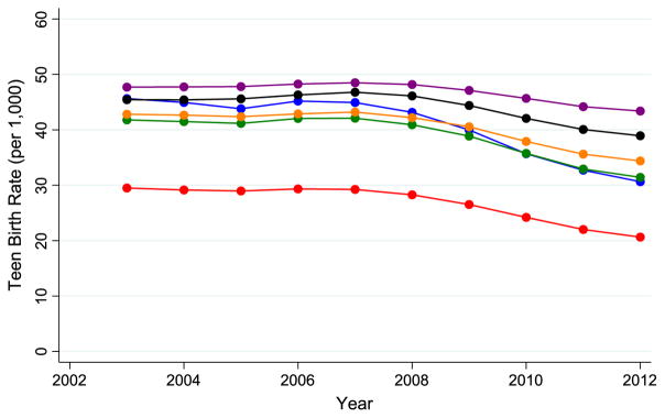
Looking at the declines in TBRs by census region, the South had the highest TBRs over the study period and the Northeast had the lowest. In 2003, the West had slightly higher TBRs than the Midwest (both in the middle between the South and Northeast) but TBRs converged for these two regions over the study period such that they were the same in 2012 (Fig. 13). Looking at the declines by urban–rural category, the lowest TBRs were observed for the large fringe counties and the highest for the non-core or rural counties throughout the study period (Fig. 14). The largest declines appeared for large central cities, from 2006 to 2012 (Fig. 15).

Fig. 13.

Trends in the predicted TBRs (per thousand) from the convolution model over time by census region: , Midwest; , Northeast; , South; , West

Fig. 14.

Trends in predicted TBRs (per thousand) from the convolution model over time by urban–rural classification: , large central; , large fringe; , medium metro; , small metro; •, micropolitan; , non-core

Fig. 15.

Trends in predicted TBRs (per thousand) from the convolution model over time by division: , East North Central; , East South; , Mid-Atlantic; , Mountain; •, New England; , Pacific; , South Atlantic; , West North Central; , West South Central

5. Discussion

Consistent with prior research, we found higher TBRs across counties in the southern USA and lower TBRs in New England counties during the study period, 2003–2012. Whereas TBRs declined across all regions of the country from 2003 to 2012, TBRs remained in excess of 80 births per 1000 adolescent females in several counties across west Texas and along the Mississippi River, as well as parts of Georgia and Alaska. In 2012, 50.1% of counties had TBRs in excess of 36 births per 1000 adolescent females (p > 0.95): our chosen exceedance threshold. Studies by Kearney and Levine (2011, 2012), National Campaign to Prevent Teen and Unplanned Pregnancy (2013) and Ventura et al. (2014) show similar geographic patterns and changes in state level TBRs, with birth rates higher in the southern and south-western regions of the USA and declining for all states over several recent decades. Prior studies such as Kuang and Williams (2013) and Chang et al. (1998) have identified risk factors that are associated with teen pregnancy such as lower income, unemployment, parents with low levels of education and smoking, drug and alcohol abuse issues. Our analysis also found that socio-economic and demographic characteristics were associated with TBRs at the county level, and that the inclusion of these factors in the models accounted for some of the spatial auto-correlation that is observed in TBRs. The geographic variation in teen births was consistent with what has been published by the Division of Vital Statistics at the National Center for Health Statistics at the state level (Hamilton and Ventura, 2012; Mathews et al., 2010; Ventura et al., 2014). Also lending credibility to the model estimates is the finding that the state level direct estimates of TBRs corresponded very closely to the model-based estimates of state TBRs. Generally, the model-based estimates were within 1% of the direct state estimates.

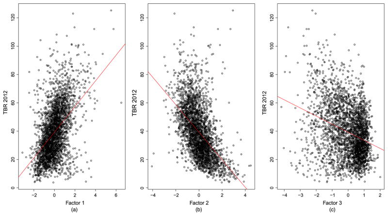
The posterior MCMC output from WinBUGS for the parameter estimates from the basic model is shown in Table 3, which shows that all the three orthogonal components were significantly associated with TBRs. The correlation of TBRs for the year 2012 with the three factors are also shown in Fig. 16. The γ-coefficients correspond to the three orthogonal component scores from the principal component analysis. Although the orthogonal component scores did not substantially improve the model fit in terms of the DIC, they did facilitate model convergence, improved the posterior distributions of the variance parameters in terms of smoothed density plots, lowered auto-correlation and were found to be significantly associated with TBRs. The uncertainty around the component scores, however, was not explicitly accounted for in the model. Incorporating this uncertainty may have an influence on the posterior predictions, parameter estimates and 95% Bayesian credible intervals; further methodological work on how best to propagate this uncertainty from the principal component analysis throughout the hierarchical Bayesian models and the corresponding effect on results would be instructive. Higher TBRs in 2003 (see Fig. 8) and in 2012 (see Fig. 9) occur in areas where poverty is high and income is low (see Fig. 1 (darker areas)), areas with low education (see Fig. 3 (lighter areas)) and a lower percentage of the population being white (see Fig. 2 (lighter areas)).

Fig. 16.

Scatter plot of TBRs with the three orthogonal component scores and the scatter plot for the three orthogonal component scores with each other: (a) R = 0.496; (b) R = −0.631; (c) R = −0.313

The limitations of this analysis are as follows. Although several models were implemented and evaluated, ranging in complexity, it is possible that alternative models incorporating different covariates or using different specifications would have improved model fit or prediction. The MCMC simulations were extremely computationally intensive, requiring an average of 6 weeks to run on a 150-Gbyte machine, which is a major limiting factor in exploring alternative models. Additionally, the exceedance probabilities are sensitive to the threshold that is selected, and alternative thresholds might be of interest. The threshold that we selected is somewhat arbitrary, but our objective was to demonstrate how this method could be used to examine county level variation in meeting specified public health objectives. Finally, there may be variation in TBRs at the subcounty level, but this variation cannot currently be explored by using data from the national vital statistics system.

The strengths of this analysis include the combination of a detailed geographic focus (at the county level), over a substantive period of time, accounting for selected factors that affect teen births, including level of education, income, poverty and race distribution. To date, most of the work on estimating TBRs and assessing geographic variation has been done at the state level (Hamilton et al., 2016; Ventura et al., 2014). County level analyses have largely not been undertaken because of the potential instability of the direct estimates at this level, which are a greater problem for counties that are sparsely populated. This study is the first to address county level variation in TBRs over time by using the BYM model to obtain smoothed, reliable estimates. The BYM model accounted for spatial and temporal dependence along with space–time interaction terms in generating county level estimates. The BYM model was enhanced by the inclusion of the three principal component scores—income and poverty, education and race or ethnicity—which were significantly associated with TBRs at the county level. In substantive terms, these findings can provide important insight into the trends and changing patterns of teen childbearing in the USA which are not afforded by an examination of national or state rates and not possible with an examination of the direct county level birth rates. Areas were identified in this paper where the estimated TBR was shown to be significantly higher than that of surrounding areas over time. Moreover, these areas were found not only within a state but across borders between states. Results from this study may aid policy makers and researchers in targeting teen pregnancy prevention programmes to areas in greatest need. This paper contributes to the existing literature by applying an existing methodology, the BYM model, to shed light on small-scale geographic variation in birth rates. This method could be applied to a variety of outcomes of public health or demographic significance for small geographic areas taking into account the spatial auto-correlation and time and space effects.

6. Conclusions and future research

The Bayesian space–time interaction models that were employed here allow the estimation of county level TBRs and an examination of how geographic patterns have changed over time. Results of this analysis suggest that 37% of counties evidenced TBRs in excess of 36 births per 1000 adolescent females in 2012 (p > 0.95). In contrast, TBRs declined for 80% of counties over the study period, with 36% of counties achieving TBRs lower than the exceedance threshold of 36 births per 1000 adolescents (p < 0.05). This approach may be valuable to monitor spatiotemporal trends in TBRs and related public health issues, as well as to evaluate whether counties have met or exceeded the national average or other targets.

Results may inform future research seeking to understand spatiotemporal patterns in teen births better and to target efforts to reduce TBRs in areas where they remain high. Given differences in TBRs across racial or ethnic subpopulations and specific age ranges such as 15–17 and 18–19 years, further examination of spatiotemporal patterns for these specific subgroups may be of interest. Work is under way to examine hot and cold spots in TBRs as well as spatial outliers (Khan et al., 2015), methods which can provide additional insight about geographic patterns and how they may have changed over time. Future work will include additional data years 2013 and 2014. Future studies on how best to propagate the uncertainty in covariates throughout the models and how findings may or may not be robust to alternative model specifications, as well as how results from these models compare with other less computationally intensive methods, may be valuable in informing future work. Together, this line of research can help to highlight areas of the country where teen births remain elevated or areas that have shown evidence of success in reducing teen births.

Appendix A: Prior assumptions: spatial model

1. α₀ is assigned an improper flat prior

   $${\alpha }_0~\text{dflat}(·).$$ (8)
2. The prior for a₁ is

   $$a_1~N(0,{\tau }_{a_1})$$ (9)
   where

   $${\tau }_{a_1}~\text{IG}(0.01,0.01).$$ (10)
3. $${\psi }_{i,t}~N({\psi }_{i,t-1},{\tau }_{\psi }),$$ (11)
   where

   $${\psi }_{i,1}~N(0,{\tau }_{\psi }),$$ (12)
   and

   $${\tau }_{\psi }~\text{IG}(0.01,0.01).$$ (13)

   The prior for type II random-walk interaction is defined above and can be regarded as a form of residual (Lawson (2013) (chapter 12) and Knorr-Held and Rasser (2000)).

4. $$\gamma ~N(0,{\tau }_{\gamma }),$$ (14)
   where

   $${\tau }_{\gamma }~\text{IG}(0.01,0.01).$$ (15)
5. The intrinsic conditionally auto-regressive prior for u_i|u_−i is

   $$u_i\mid u_{-i}~N({\overline{u}}_i,{\tau }_u/n_{{\delta }_i})$$ (16)
   and is termed correlated heterogeneity (variability), where

   $$\begin{array}{c}{u}_{-i}=(u_1,u_2,\dots ,u_{i-1},u_{i+1},\dots ,u_m),\\ {\overline{u}}_i=\sum _{j=1}^m{\omega }_{ij}{u}_j/\sum _{j=1}^m{\omega }_{ij},\end{array}$$ (17)
   δ_i is the neighbourhood of the ith region, nδ_i is the number of neighbours, ${\sum }_{j=1}^m{\omega }_{ij}$ and ω_ij equals 1 for counties i and j that are deemed neighbours and otherwise 0. We used the K -nearest-neighbours approach to define the spatial relationships between counties. The eight closest neighbours to the target county were assigned weights ω_ij = 1; all other counties are assigned weights ω_ij = 0. τ_u is the variance:

   $${\tau }_u~\text{IG}(0.01,0.01).$$ (18)
6. The prior for v_i is

   $$v_i~N(0,{\tau }_v)$$ (19)
   and is termed uncorrelated heterogeneity (variability), where τ_v is the variance and τ_v is assigned the prior

   $${\tau }_v~\text{IG}(0.01,0.01).$$ (20)
   Prior assumptions: for the non-spatial model

   $${\mathit{\beta }}_i=({\beta }_{1i},{{\beta }_{2i})}^{\prime },$$ (21)

   $${\mathit{\beta }}_i\stackrel{\text{IID}}{\sim }N(\mathbf{\mu },\mathbf{\Upsilon }).$$ (22)
   The hyperprior for μ is assumed to be distributed as

   $$N\left\{\left(\begin{array}{c}0\\ 0\end{array}\right),\left(\begin{array}{cc}{10}^{-6}& 0\\ 0& {10}^{-6}\end{array}\right)\right\}.$$ (23)
   The inverse of ϒ is assigned a Wishart prior with R as a diagonal matrix and degrees of freedom 2:

   $$\text{Wish}\left\{\left(\begin{array}{cc}0.1& 0\\ 0& 0.1\end{array}\right),2\right\}.$$ (24)

References

- Ando T. Bayesian Model Selection and Statistical Modeling. New York: Chapman and Hall; 2010. [Google Scholar]
- Barker LE, Thompson TJ, Kirtland KA, Boyle JP, Geiss LS, McCauley MM, Albright AL. Bayesian small area estimates of diabetes incidence by United States county, 2009. J Data Sci. 2013;11:249–267. [PMC free article] [PubMed] [Google Scholar]
- Besag J, Kooperberg C. On conditional and intrinsic autoregressions. Biometrika. 1995;82:733–746. [Google Scholar]
- Besag J, York J, Mollié A. Bayesian image restoration, with two applications in spatial statistics. Ann Inst Statist Math. 1991;43:1–20. [Google Scholar]
- Bivand R, Altman M, Anselin L. Package spdep. 2014. [Google Scholar]
- Böhning D, Dietz E, Schlattmann P. Space-time mixture modelling of public health data. Statist Med. 2000;19:2333–2344. doi: 10.1002/1097-0258(20000915/30)19:17/18<2333::aid-sim573>3.0.co;2-q. [DOI] [PubMed] [Google Scholar]
- Brown P, Zhou L. MCMC for generalized linear mixed models with glmmbugs. R J. 2010;2:13–17. [Google Scholar]
- Carlin BP, Louis TA. Bayesian Methods for Data Analysis. New York: Chapman and Hall; 2009. [Google Scholar]
- Chang P, Chisholm R, Bennett N, McViem M. National Initiative on Teenage Pregnancy. American Medical Student Association; Reston: 1998. [Google Scholar]
- Curtin SC, Joyce AM, Ventura SJ, Henshaw SK. Data Brief. National Center for Health Statistics; Hyattsville: 2013. Pregnancy rates for U.S. women continue to drop; p. 136. (Available from http://www.cdc.gov/nchs/data/databriefs/db136.pdf.) [PubMed] [Google Scholar]
- Dennison C. Teenage pregnancy: an overview of the research evidence. Health Development Agency; Wetherby: 2004. (Available from http://www.gserve.nice.org.uk/nicemedia/documents/teenpreg_evidence_overview.pdf.) [Google Scholar]
- Environmental Systems Research Institute. ArcGIS Desktop: Release 10. Redlands: Environmental Systems Research Institute; 2011. [Google Scholar]
- Furrer R, Sain SR. SPAM: a sparse matrix R package with emphasis on MCMC methods for Gaussian Markov random fields. J Statist Softwr. 2010;36:1–25. [Google Scholar]
- Gelfand AE, Ghosh SK. Model choice: a minimum posterior predictive loss approach. Biometrika. 1998;1:1–11. [Google Scholar]
- Gelman A. Prior distributions for variance parameters in hierarchical models (comment on article by Browne and Draper) Baysn Anal. 2006;1:515–533. [Google Scholar]
- Gelman A, Carlin JB, Stern SH, Rubin DB. Bayesian Data Analysis. New York: Chapman and Hall; 1995. [Google Scholar]
- Griffin JE, Brown PJ. Inference with normal-gamma prior distributions in regression problems. Baysn Anal. 2010;5:171–188. [Google Scholar]
- Guttmacher Institute. Needs & services, US county tables. Guttmacher Institute; New York: 2010. [Google Scholar]
- Hamilton BE, Martin JA, Osterman MJK. Births: preliminary data for 2015. Natn Vitl Statist Rep. 2016;65(3) [PubMed] [Google Scholar]
- Hamilton BE, Ventura SJ. Data Brief 89. National Center for Health Statistics; Hyattsville: 2012. Birth rates for US teenagers reach historic lows for all age and ethnic groups. [PubMed] [Google Scholar]
- Health Resources and Services Administration. Area health resources file. Health Resources and Services Administration; Rockville: 2012. (Available from http://ahrf.hrsa.gov/download.htm.) [Google Scholar]
- Ingram DD, Franco SJ. NCHS urban-rural classification scheme for counties. Vitl Hlth Statist. 2012;2:1–65. [PubMed] [Google Scholar]
- Kearney MS, Levine PB. Working Paper 17157. National Bureau of Economic Research; Cambridge: 2011. Income inequality and early nonmarital childbearing: an economic exploration of the culture of despair. [Google Scholar]
- Kearney MS, Levine PB. Working Paper 17964. National Bureau of Economic Research; Cambridge: 2012. Explaining recent trends in the U.S. teen birth rate. [Google Scholar]
- Khan D, Rossen LM, Dienes E, He Y, Hamilton BE, Wei R. Working Paper. National Center for Health Statistics; Hyattsville: 2015. Hot spots, cluster detection and outlier analysis of teen birth rates in the U.S., 2003–2012. [Google Scholar]
- Kirby D, Lepore G, Ryan J. Sexual risk and protective factors: factors affecting teen sexual behavior, pregnancy, childbearing, and sexually transmitted disease: which are important?; which can you change? Washington DC: National Campaign to Prevent Teen and Unplanned Pregnancy; 2005. (Available from https://thenationalcampaign.org/sites/default/files/resource-primary-download/protective_factors_full.pdf.) [Google Scholar]
- Knorr-Held L, Besag J. Modelling risk from a disease in time and space. Statist Med. 1998;17:2045–2060. doi: 10.1002/(sici)1097-0258(19980930)17:18<2045::aid-sim943>3.0.co;2-p. [DOI] [PubMed] [Google Scholar]
- Knorr-Held L, Rasser G. Bayesian detection of clusters and discontinuities in disease maps. Biometrics. 2000;56:13–21. doi: 10.1111/j.0006-341x.2000.00013.x. [DOI] [PubMed] [Google Scholar]
- Kost K, Henshaw S. U.S. Teenage Pregnancies, Births and Abortions, 2008: National Trends by Age, Race and Ethnicity. New York: Guttmacher Institute; 2012. (Available from http://www.guttmacher.org/pubs/USTPtrends08.pdf.) [Google Scholar]
- Kost K, Henshaw S, Carlin L. U.S. Teenage Pregnancies, Births and Abortions: National and State Trends and Trends by Race and Ethnicity. New York: Guttmacher Institute; 2010. (Available from http://www.guttmacher.org/pubs/USTPtrends.pdf.) [Google Scholar]
- Kuang C, Williams K. Investigating risk factors affecting teenage pregnancy rates in the United States. Eur Int J Sci Technol. 2013;2(2) [Google Scholar]
- Lagazio C, Dreassi E, Biggeri A. A hierarchical Bayesian model for space-time variation of disease risk. Statist Modllng. 2001;1:17–29. [Google Scholar]
- Lawson A. Bayesian Disease Mapping: Hierarchical Modeling in Spatial Epidemiology. Boca Raton: Chapman and Hall–CRC; 2013. [Google Scholar]
- Lee D. CARBayes: an R package for Bayesian spatial modeling with conditional autoregressive priors. J Statist Softwr. 2013;55(13):1–24. [Google Scholar]
- Lunn D, Jackson C, Best N, Thomas A, Spiegelhalter D. The BUGS Book: a Practical Introduction to Bayesian Analysis. Boca Raton: Chapman and Hall–CRC; 2013. [Google Scholar]
- Martin JA, Hamilton BE, Osterman MJ, Ventura SJ, Mathews T. Births: final data for 2011. Natn Vitl Statist Rep. 2015;62:1–90. [PubMed] [Google Scholar]
- Mathews TJ, Sutton PD, Hamilton BE, Ventura SJ. Data Brief 46. National Center for Health Statistics; Hyattsville: 2010. State disparities in teenage birth rates in the United States. [PubMed] [Google Scholar]
- National Campaign to Prevent Teen and Unplanned Pregnancy. Counting it up: the public costs of teen childbearing: key data. National Campaign to Prevent Teen and Unplanned Pregnancy; Washington DC: 2013. (Available from https://thenationalcampaign.org/resource/counting-it-key-data-2013.) [Google Scholar]
- National Center for Health Statistics. Bridged-race intercensal population estimates. National Center for Health Statistics; Hyattsville: 2012. (Available from http://www.cdc.gov/nchs/nvss/bridged_race/data_documentation.htm#july2009.) [Google Scholar]
- National Latino Research Center. Prevent teen and unplanned pregnancy: the National Campaign to Prevent Teen and Unplanned Pregnancy; counting it up; the public costs of teen childbearing; key data. National Latino Research Center; 2005a. (Available from http://thenationalcampaign.org/sites/default/files/resource-primary-download/what-policymakers-can-do.pdf.) [Google Scholar]
- National Latino Research Center. Teen pregnancy among latinas in San Diego County: contraceptive and abortion attitudes and behavior. National Latino Research Center; 2005b. (Available from http://www.csusm.edu/nlrc/documents/Fact_Sheet_Teen_Pregnancy.pdf.) [Google Scholar]
- Ntzoufras I. Bayesian Modeling using Winbugs. Hoboken: Wiley; 2009. [Google Scholar]
- Penman-Aguilar A, Carter M, Snead MC, Kourtis AP. Socioeconomic disadvantage as a social determinant of teen childbearing in the U.S. Publ Hlth Rep. 2013;128:5–22. doi: 10.1177/00333549131282S102. [DOI] [PMC free article] [PubMed] [Google Scholar]
- Population Reference Bureau. U.S. teen birth rate correlates with state income inequality. Population Reference Bureau; Washington DC: 2012. (Available from http://www.prb.org/Publications/Articles/2012/us-teen-birthrate-income.aspx.) [Google Scholar]
- Rao J, Yu M. Small-area estimation by combining time-series and cross-sectional data. Can J Statist. 1994;22:511–528. [Google Scholar]
- Shoff C, Yang T. Spatially varying predictors of teenage birth rates among counties in the United States. Demogr Res. 2012;27:377–418. doi: 10.4054/DemRes.2012.27.14. [DOI] [PMC free article] [PubMed] [Google Scholar]
- Spiegelhalter DJ, Best NG, Carlin BP, van der Linde A. Bayesian measures of model complexity and fit (with discussion) J R Statist Soc B. 2002;64:583–639. [Google Scholar]
- Spiegelhalter D, Thomas A, Best N, Lunn D. Winbugs User Manual. Cambridge: Medical Research Council Biostatistics Unit; 2003. [Google Scholar]
- Tipping ME, Bishop CM. Probabilistic principal component analysis. J R Statist Soc B. 1999;61:611–622. [Google Scholar]
- Ventura SJ, Hamilton BE, Mathews TJ. National and state patterns of teen births in the United States, 1940–2013. Natn Vitl Statist Rep. 2014;63(4) [PubMed] [Google Scholar]
- Wall MM. A close look at the spatial structure implied by the CAR and SAR models. J Statist Planng Inf. 2004;121:311–324. [Google Scholar]
- Xia H, Carlin BP, Waller LA. Hierarchical models for mapping Ohio lung cancer rates. Environmetrics. 1997;8:107–120. [Google Scholar]
Associated Data
This section collects any data citations, data availability statements, or supplementary materials included in this article.