The mechanism of force transmission at bacterial focal adhesion complexes

Summary

Various rod-shaped bacteria mysteriously glide on surfaces in the absence of appendages such as flagella or pili. In the deltaproteobacterium Myxococcus xanthus, a putative gliding motility machinery (Agl–Glt) localizes to so-called Focal Adhesion sites (FA) that form stationary contact points with the underlying surface. We discovered that the Agl–Glt machinery contains an inner-membrane motor complex that moves intracellularly along a right-handed helical path, and when it becomes stationary at FA sites, it powers a left-handed rotation of the cell around its long axis. At FA sites, force transmission requires cyclic interactions between the molecular motor and adhesion proteins of the outer membrane via a periplasmic interaction platform, which presumably involves a contractile activity of motor components and possible interactions with the peptidoglycan. This work provides the first molecular model for bacterial gliding motility.

Introduction

Certain rod-shape bacteria move along their long axis in the absence of extracellular appendages, such as flagella or pili, in a process called gliding motility¹. In Myxococcus xanthus gliding is mediated by bacterial Focal Adhesion sites (FA). During gliding motility, FA sites assemble at the leading cell pole and retain a fixed position relative to the surface until they disassemble at the lagging cell pole¹. FA sites contain a molecular machinery, named Agl-Glt, containing more than fourteen proteins^2–4. Genetic analysis suggested that this machinery is formed by two membrane-associated machineries: (i), a putative three protein TolQR-like Proton Motive Force (PMF)-driven channel (AglR,Q,S) –the suspected energy producing system^3,5,6; and (ii), a putative eleven-protein integral envelope-associated complex (GltA-K) that interacts with the Agl system^2–4. These machineries are further connected to a cytosolic protein complex formed by the AglZ protein, the Ras-like G-protein MglA and the MreB actin cytoskeleton (hereafter MreB complex⁷, Figure 1a). This MreB complex recruits, and promotes the assembly of the Agl-Glt machineries (Figure 1a). Directional Agl-Glt movements from the leading towards the lagging cell pole were suggested to propel the cell forward^3,8, but how these movements may be transduced into cell movement remains unknown^5,9. Here, we reveal the functional architecture of the Agl-Glt complex and establish how its activity is transduced to the contact surface across the highly structured layers of the cell envelope.

Figure 1. The Myxococcus motility complex moves directionally along a helical path.

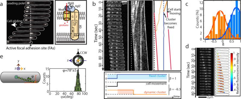
(a) Spatial regulation of the Myxococcus motility complex. A motile AglZ-YFP expressing cell showing a complete assembly cycle is shown at 30 s time intervals. A current view of an Agl (blue)-Glt (yellow) complex at a focal adhesion site (FA) is shown^2,7,19. Assembly occurs at the leading cell pole following interactions between MglA-GTP, MreB and AglZ (right panel, blue,⁸). The position of the Glt proteins is drawn based on published works^2–5,7,20.

(b) Immobilization of AglZ-YFP clusters correlates with cell movement. TIRFM of AglZ-YFP in a cell that shifts to motility on a chitosan-treated surface. Images were acquired every 0.5 s. Selected time frames and the corresponding high-resolution kymograph are shown. Two dynamic (orange) clusters are shown. Note that cell movement (indicated by the dashed line showing the initial cell position) is only observed when a cluster becomes stationary (see orange/blue cluster). Scale bar = 2 μm. Lower panel: calculation of the correlation coefficient (ß) between the presence of a cluster and cell movement. The fixed cluster (blue) is highly correlated with cell movement (ß=1), whilst the dynamic cluster (orange) is partially anti-correlated (ß=−0.3).

(c) Distribution of the correlation coefficient ß for fixed (blue) and dynamic clusters (orange), n=95 (6 biological replicates).

(d) AglZ-YFP clusters move along helical trajectories. TIRFM selected time frames of a dynamic AglZ-YFP cluster in a non-motile cell are shown. Scale bar = 2 μm.

(e) Measurement of the trajectory angle (φ_A) from n= 54 (8 biological replicates) single trajectories of dynamic AglZ-YFP clusters (top panels). Histogram of φ_Aand Gaussian fit (grey line) are in the panel below. The mean angle is shown with a dashed vertical line and corresponds to counterclockwise trajectories.

Results

We quantitatively characterized the dynamic behavior of FA sites by analyzing the motions of AglZ-YFP-containing complexes using Total Internal Reflection Fluorescence Microscopy (TIRFM). Cells attached to a chitosan-coated surface alternated between motile and non-motile states. In these conditions, we were able to capture the movement of AglZ-YFP clusters over extended periods of time with high temporal resolution. Two main AglZ-YFP cluster populations were observed: static and dynamic (Figure 1b, blue and orange, respectively). Motile cells on chitosan exhibited at least one AglZ-YFP static cluster, indicating that a single static cluster is necessary and sufficient for cell propulsion. We also observed dynamic AglZ-YFP clusters. These clusters tended to form at the cell pole and migrate directionally towards the opposite pole (Figure 1b, Extended Figure 1a). On average, clusters formed every minute and moved at constant velocity (3.2 ± 0.9 μm/min, n=227) over distances of 1.5 ± 1 μm (n=203), often becoming dissociated upon reaching the opposite pole. Cluster speeds varied within and between cells (Extended Figure 1b), possibly due to varying numbers of motor units in a cluster (see below) and varying PMF levels between cells^3,6. Dynamic clusters likely represent unattached motility complexes because: (i) in motile cells, they were only detected if a fixed cluster was also present and (ii), in most cells the transition from a non-motile to a motile state coincided with cluster immobilization (>85%, n=34, Figure 1b, orange-blue cluster). To quantitatively characterize this behavior, we measured the correlation ß between cell movement and presence of static and dynamic clusters (Figure 1b, lower panel). Importantly, presence of static -but not dynamic-clusters was highly correlated with cell movement (Figure 1c, n=95).

Close examination of dynamic clusters by TIRF revealed that they not only move between poles but they also move across the cell width following a helical path (Figure 1d). The helicity, characterized by φ_A, the angle representing the pitch of a helix when projected on a plane (Figure 1e), was constant between cells (78°±5, n=54, Figure 1e). In most cases (92%, n=54), the direction of rotation of AglZ-YFP clusters relative to the direction of movement was counterclockwise (CCW), denoting a right-handed helical path. Treating the cells with A22, a drug that inhibits MreB polymerization¹⁰, decreased the number of dynamic clusters per cell (Extended Figure 1c–d) but notably not their helical movement and directionality (Extended Figure 1e).

We reasoned that if propulsion was linked to the counterclockwise trafficking of AglZ-YFP-containing motility complexes, then a gliding cell body should rotate along a similar helical path but of opposite handedness (i.e. clockwise or CW, Figure 2a). To test this, we followed the dynamics of fiducial markers (artificial fluorescent D-Amino Acids, or TADA) fixed to the cell periphery during cell movement (Extended Data Figure 2a–d). In motile cells, TADA clusters moved from one side to the opposite side of the cell with angular velocities proportional to the speed of motility (Figure 2b, Extended Data Figure 2e), consistent with TADA clusters reporting on the overall rigid-body rotational movement of the cell during propulsion.

Figure 2. Myxococcus cells rotate during motility.

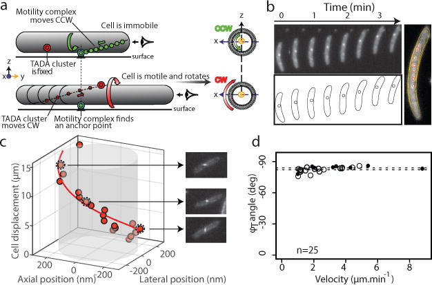
(a) The helical movement of intracellular motors predicts rotation of the cell during movement.

(b) Rotation of a TADA-bright cluster in a motile cell (30s intervals) and in a sum-type projection (right). The cartoon representation shows the position of the centroid of the cluster relative to the cell outline.

(c) 3D positions of a TADA-bright cluster measured by astigmatism (orange dots) illustrating the clockwise rotation of the motile cell (n=8 ; 5 biological replicates). Snapshots of the cell are displayed, illustrating the deformation of the PSF as a function of the axial position.

(d) Rotation angle of TADA-bright clusters (φ_T) as a function of cell velocity from astigmatism (filled circles, 83.9° ± 2.5 n=8 ; 5 biological replicates) and intensity variations (open circles 82.0° ± 2.6 n=17 ; 3 technical replicates).

To determine the direction of rotation, we directly tracked the 3D position of TADA clusters during cell movement by inducing astigmatism into the optical detection path¹¹ (Methods). In agreement with our predictions, TADA clusters rotated in the clockwise direction during cell propulsion (Figure 2c, Extended Data Figure 2f, n=8). These observations were confirmed by monitoring fluorescence intensity fluctuations with respect to the imaging focal plane during cell movement (Methods, Extended Data Figure 2g, n=17). The rotation angle for TADA clusters (φ_T) was constant between cells (82.6 ± 2.7 ° n=25, as measured by both methods, Figure 2d) and closely matched the angle of rotation (φ_A) measured for AglZ-YFP clusters (78°±5). Interestingly, φ_T did not vary significantly with cell speed (Figure 2d). Altogether, these findings suggest that anchoring of dynamic AglZ-YFP containing complexes leads to the clockwise rotation of the cell and its forward propulsion.

To gain further insight into the molecular mechanism of motility, we genetically dissected the functional groups composing the Agl-Glt machinery (Figure 1a). Notably, mutations in agl and glt genes led to aberrant localization patterns and perturbation of AglZ-YFP cluster dynamics (Figure 3a, Extended Data Figure 3a). The global effect of each mutant in the localization pattern of AglZ-YFP was evaluated by measuring four observables: the proportion of cells exhibiting clusters, the mean number of AglZ-YFP clusters, and their longitudinal and radial distributions for wild-type and mutant cells (Figure 3a, Extended Data Figure 3b). Principal component analysis (PCA) was used to quantitatively characterize the effect of each mutant in the assembly of AglZ-YFP clusters (Methods). This statistical method allowed us to convert the set of correlated observables into a set of linearly uncorrelated principal components (PCs).

Figure 3. Functional architecture of the Agl-Glt machinery.

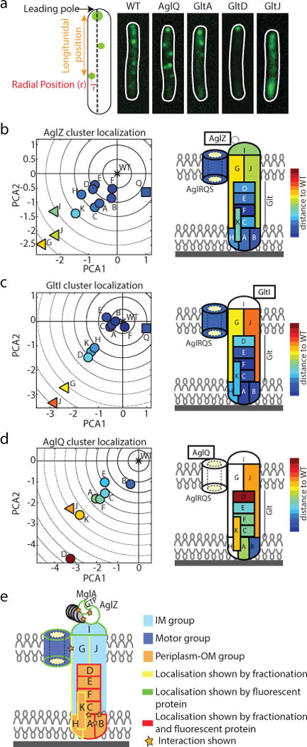
(a) The localization of AglZ-YFP is affected to different extents in agl-glt mutants. The number and position (longitudinal and radial) of clusters was determined in each mutant background and their effect analyzed by PCA (see Methods). Scale bar = 1 μm.

(b–d) The effect of mutations in assembly dynamics of AglZ-YFP, GltI-YFP and AglQ-mCherry plotted in PC coordinates. Triangles represent IM group proteins, squares motor components and circles the rest (periplasm-OM). Right panels show schematic representations of the projections of the defined gene groups with respect to their predicted/shown localization from^2–5,7,20. Color code represents distance to the WT in PC space. Letters represent each protein subunit of the Agl/Glt complex.

(e) The compilation of PCA (panels b-d) superimposed to available data^2–5,7,20 suggests that the motility machinery consists of a molecular motor (dark blue), an IM-cytosolic group (light blue) and a large periplasm-OM group (orange).

The first three PCs described >87% of the variance (Extended Data Figure 4a–d). PC1 represented a linear combination of the number of AglZ-YFP clusters, longitudinal cluster position, and proportion of cells with clusters. PC2 mostly represented the average number of clusters detected per cell, while PC3 was essentially dominated by the mean radial cluster position (Extended Data Figures 4a–d). A synthetic representation of results can be obtained by plotting the mean position of each mutant in a PC space where the wild-type (WT) is arbitrarily positioned at the origin (Figure 3b; for clarity only PC1 and PC2 are shown but the analysis is computed from PC1-3, Extended Data Figure 4e). Therefore, for each mutant, the distance to the origin and the direction represent the relative effect of a mutation on the number and distribution of AglZ-YFP clusters. Predicted inner membrane (IM) components (IGJ) exhibited the largest perturbation in the assembly dynamics of AglZ-YFP clusters, while periplasmic-outer-membrane (OM) group proteins (ACDEHK) displayed the lowest effect (Figure 3b). Interestingly, AglQ (motor) affected AglZ-YFP cluster formation in a qualitatively different manner, represented by a direction in PC space orthogonal to that observed for other mutants.

We refined the functional connections between agl-glt genes by further investigating the impact of gene deletions in the formation of GltI-YFP⁷ and AglQ-mCherry^3,7 clusters, putative cytosolic and motor components of the gliding machine. The overall effect of gene deletions in the number and distribution of GltI-YFP clusters was similar to that observed for AglZ-YFP, consistent with GltI and AglZ belonging to the same functional group (Figure 3c). GltJ and GltG, two predicted IM proteins² and thus possibly in direct contact with GltI, had a large effect on GltI-YFP assembly (Figure 3c). Interestingly, GltD, GltH and GltK exhibited a larger impact than other proteins in their subgroup (e.g. A,B,C,E), suggesting that direct protein-protein interactions between these proteins and factors of the GltI subgroup may be needed for GltI-YFP localization (Figure 3c). Finally, we analysed the effect of deletions in the assembly of motor components (AglQ). Strikingly, deletion of factors in all subgroups led to severe perturbations in the formation of AglQ-mCherry fluorescent clusters (Figure 3d), suggesting that the motor may require several contacts with different Glt proteins to form functional clusters. However, specific components exhibited differential roles: GltJ, D and K displayed the largest effects, while GltB barely affected formation of AglQ clusters (Figure 3d). Overall, this data indicate that the motility complex is divided into several distinct functional groups (Figure 3e).

To determine the sequence of events leading to the assembly of propulsive complexes, we imaged the dynamic localization of AglZ-YFP (cytosolic-IM group) simultaneously with that of proteins belonging to each of the other functional subgroups: AglQ (motor), GltD (periplasmic), or GltC-mCherry (peri-OM complex) (Figures 4a, 4c, 4e). By conventional epifluorescence microscopy, cytosolic (AglZ) and motor components (AglQ) in motile cells (1.5% agar) displayed a strong ability to form clusters, in contrast to the dispersed localization of periplasmic and OM complex components (GltC,D) to the cell periphery (Extended Data Figure 5a). Thus, we used TIRFM to image the dynamic localization of these factors in motile cells adhered to chitosan-coated glass. AglQ-mCherry and AglZ-YFP co-localized in both stationary and mobile clusters, indicating that these proteins form a stable complex in the bacterial IM (Figure 4a, see also Methods and Extended Data Figure 5b–c, 6). To analyze whether clusters containing both AglZ and AglQ were linked to cell motility, we calculated for each cell the correlation between cell movement and co-localization and computed the distributions for both stationary and mobile clusters (Figure 4b, see Methods and Extended data Figure 7). Interestingly, stationary clusters were highly correlated to cell movement while mobile clusters were not, consistent with AglZ and AglQ being part of the trafficking internal complex (Figure 4b). In contrast, GltD- and GltC-mCherry co-localized with AglZ-YFP only in stationary clusters (Figures 4c, e and Extended Data Figures 5b–c) and co-localization of stationary AglZ-GltC/D clusters was highly correlated to cell movement (Figures 4d, f). These data strongly suggest that cytosolic-IM and motor complexes assemble together in a mobile unit that requires a physical connection to periplasmic and OM components to form stationary clusters that impart cell movement.

Figure 4. Dynamic interactions between the intracellular and outer-membrane complexes generate propulsion.

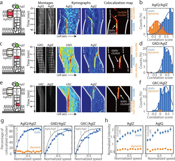
(a) Simultaneous dynamics of AglZ-YFP and AglQ-mCherry and correlation to the motility phases. TIRFM images of a time lapse and corresponding kymographs are shown for individual fluorescent fusions and in a heat map showing the computed co-localization scores.

(b) AglZ and AglQ co-localize in the IM trafficking complex (n=156 cells ; 2 biological replicates). Correlations scores reflect the correlation between cell movement and static co-localized clusters.

(c–d) Simultaneous dynamics of AglZ-YFP and GltD-mCherry and correlation to the motility phase (n=121 cells ; 7 biological replicates). Legend reads as in a–b.

(e–f) Simultaneous dynamics of AglZ-YFP and GltC-mCherry and correlation to the motility phase (n=100 cells ; 3 biological replicates). Legend reads as in a–b.

(g) Correlation between cell velocity and number of active complexes. For a given value of the cell speed (V), the percentage of co-localized clusters represents the proportion of events where a cell was moving at speed V and an active cluster containing both AglZ and AglQ/GltD/GltC was detected. The percentage of co-localization is shown as a function of normalized cell speed (where 1 is the maximum cell speed).

(h) Correlation between cell velocity and intensity of AglZ and AglQ clusters. Intensity was normalized with respect to the average intensity measured for dynamic clusters and shown as a function of normalized cell speed. Error bars represents the standard error of the mean and was calculated according to the total number of cells analyzed (n=114 cells for AglZ, n=100 for AglQ).

To further investigate this hypothesis, we determined the correlation between cell speed and the proportion of clusters containing both AglZ and AglQ/GltC/GltD (Figure 4g). Dynamic clusters containing AglZ and AglQ were observed in motile cells, however their number was independent of cell speed, indicating that they are not propulsive by themselves (Figure 4g). On the contrary, the proportion of AglZ/AglQ clusters being stationary rapidly increased with cell speed (Figure 4g). Interestingly, the number of AglZ/AglQ clusters reached a maximum at ∼50% of the cell maximum speed (V_1/2), suggesting that this number is not a limiting factor (Figure 4g). In fact, the recruitment of GltD and GltC to FA sites could be a limiting step because a significant number of static AglZ clusters lack GltD and especially, GltC (Extended Data Figure 5b–c). Consistent with this, the number of stationary AglZ/GltD and AglZ/GltC clusters was only ~60% of the maximum at V_1/2 and full speed was only reached when the percentage of GltD/GltC stationary clusters recruited to FA sites saturated (Figure 4g). Thus, the recruitment of GltD and GltC to FA sites is required for propulsion likely because these proteins belong to complexes that link the motor to the external surface.

To further test whether the stoichiometry of Agl-Glt components regulates the activity of FA sites, we measured how the mean fluorescence intensity of stationary and mobile clusters changed with normalized cell speed (Figure 4h, see Methods). Cell speed increased with the number of AglZ and AglQ subunits accumulating in stationary clusters while their proportion in mobile clusters was systematically lower (Figure 4h). All in all, these results show that stationary FA complexes form due to the transient recruitment of periplasmic and OM proteins by the mobile PMF-driven IM complex. Importantly, the activity of stationary complexes is regulated at two levels: by the number of Agl motor units (force generation) and by the number of local contacts with periplasmic-OM components (transmission).

A clear prediction of this model is that the motility complex should require direct adhesive contacts with the underlying surface to propulse the cell. Consistent with this, Reflection Interference Contrast Microscopy (RICM) revealed that motile cells are uniformly in contact with the substratum while high RICM densities are correlated with the position of AglZ-YFP clusters (Extended Figure 5d). Interestingly, we observed that vesicles only containing OM-materials and specific OM Glt proteins (GltC-mCherry) were deposited at sites coinciding with the position of FA complexes in the wake of motile cells (Figure 5a, Extended Data Figure 5e–f) Overall, this data suggest that adhesions involve strong intimate contacts between the surface and the periplasm-OM complex.

Figure 5. Cyclic contacts between the IM motor and OM adhesins drive propulsion.

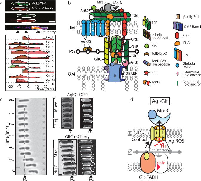
(a) GltC-mCherry, is released by gliding cells at FA complexes. Upper panel - TIRFM snapshots are shown for a representative cell expressing both GltC-mCherry (red) and AglZ-YFP (green). The position of the GltC clusters on the surface coincides with position of FA complexes (white asterisk). Time frames: 15s. Scale bar = 2μm. Lower panel - variation of intensity for GltC-mcherry (red) and AglZ-YFP (green) as a function of time before (negative time) and after (positive time) the cell moved away from the FA position, shown for n=10 (2 technical replicates).

(b) Predicted domain architecture of the Agl-Glt machinery based on bioinformatics prediction, sequence analysis and previous literature. The different proteins of the complex are represented based on their domain structures from bioinformatics predictions (Supplementary Table S1). Each protein is represented as a single copy in the complex.

(c) A fixed contractile (FC) zone is observed in motile sporulating cells where peptidoglycan is profoundly remodeled. Motile cells in the early phases of sporulation are shown at 1 min intervals. AglQ-sfGFP and GltC-mCherry are specifically enriched at the constriction site. Representative cells are shown for WT (n=10), AglQ-sfGFP (n=2) and GltC-mCherry (n=4) each obtained from 2 biological replicates.

(d) Possible mechanism of propulsion. The structure of the Agl-Glt machinery is simplified to its core components for clarity. The proton flow through a PG-bound TolQR-type channel (yellow) is proposed to energize cyclic interactions between a flexible IM-anchored periplasmic protein (GltG/J, black-yellow) and TonB-box proteins in the OM (orange). Combined with the rigid anchoring to PG and link with MreB, this activity would push the OM protein laterally (red arrow) because PG counteracts the exerted traction force (grey arrow). The protein stoichiometries are not known and it is possible that the complex contains several coordinated legs, facilitating the processivity and directionality of the movements.

To gain molecular insight into the mechanisms involved in force generation and surface adhesion, we predicted a protein-domain structure of the motility complex using bioinformatics approaches (Figure 5b, Extended Data Figures 8–9). Remarkably, both AglQ and AglS contain predicted TolR-like PG-binding motifs¹² and AglR, a TolQ homolog interacts with GltG² a TolA/TonB-like protein (Extended Data Figure 8a–b). GltG and GltJ are similar modular proteins, specifically sharing a single transmembrane helix, a periplasmic helical domain, and TonBC motifs¹³. Interactions of GltGJ with OM components could occur between their TonBC domains and potential TonB-box-carrying proteins -GltF in the periplasm (Extended Data Figure 8a) and GltAB, two predicted porin-like β-barrel proteins in the OM (Extended Data Figure 9a–b).

Thus, PG-anchored Agl motor units may act as stators pushing against adhesive OM complexes through PG to generate propulsive forces. We reasoned that these dynamic interactions might be revealed under conditions where the rigidity of the cell envelope is reduced, for example in cells undergoing sporulation where rapid PG remodeling leads to the formation of round cells¹⁴. Indeed, inducing sporulation rapidly led to the formation of balloon-shaped cells (Figure 5c). Remarkably, a small fraction of cells (<1%) entering sporulation are still motile and form conspicuous constrictions that, similar to FA complexes, remained fixed relative to the surface (Figure 5c). These constrictions likely result from the activity of the Agl-Glt machinery because i), they only formed in motile sporulating cells (less than 1% of the sporulating cell population) and ii), both AglQ-sfGFP (inner membrane, or IM) and GltC-mCherry (outer membrane, or OM) were enriched at constriction sites (Figure 5c). Thus, in sporulating cells where the structure of peptidoglycan is different (PG is not detected in mature spores¹⁵) dynamic Agl-Glt-driven physical contacts between the OM and the IM are unmasked.

Discussion

Based on our results,we propose that the Agl motor and associated IM proteins move directionally by cyclic interactions with factors in the periplasmic-OM complex (Figure 5d). Analogous to Tol/Exb systems^13,16, these steps would occur by pmf-driven conformational changes in the Glt TolA/TonB-like proteins (GltG and/or GltJ, Figure 5b), the flexible-domain of which might extend and retract through the PG layer (Figure 5d). PG itself could act both as a transient anchor point, as it becomes bound by AglQ/S via the possible TolR-like PG-binding motif, and a guiding factor, opposing contractions and favoring lateral movements (Figure 5d).

The current study does not resolve the relative stoichiometries of the Agl-Glt proteins at FAs, however the data shows that the activity of FA complexes is subject to regulation, and contains variable stoichiometries of Agl motor components and connections with the underlying surface. Thus, it is possible that several “legs” operate coordinately at these sites. The directionality of motility complexes is remarkably robust between cells, suggesting a role of a core cellular structure; PG is an attractive candidate because the glycan strands are proposed to have a global right-handed helical ordering and could serve as track to guide the motility complex¹⁷. At FAs, the interaction with the surface appears to be strong, implying the existence of a specific adhesion(s) and consequently, a relief mechanism like in gliding parasites where the major adhesion is removed from the motility complex by specific proteolysis¹⁸. Excitingly, the model makes several important predictions that will help future studies, specifically guiding the exploration of protein interactions in the system, the next step towards a molecular understanding of the motility mechanism.

Methods

Bacterial Strains, Plasmids, and Growth

Strains, primers, and plasmids are listed in Extended Data Tables S2 and S3. See Extended Data Tables S2 and S4 for strains and their mode of construction. M. xanthus strains were grown at 32°C in CYE rich media as previously described¹. Plasmids were introduced in M. xanthus by electroporation. Mutants and transformants were obtained by homologous recombination based on a previously reported method¹. All fusions were expressed by gene replacement at the endogenous loci allowing expression from the natural promoters. Q-PCR experiments confirmed that expression is similar to WT levels (expression ratios varied between 1 and 2 compared to WT levels). Three types of AglQ fusions were used throughout the study, TIRF experiments used AglQ-mCherry expressed from the endogenous locus in place of the WT gene. For technical reasons, the PCA analysis and expression of AgQ-sfGFP and, used fusions expressed after ectopic integration of the gene of interest at the Mx8-phage attachment site in a ΔaglQ deletion backgrounds (Extended Data Table S4). All three strains were indistinguishable in terms of motility and expression patterns. E. coli cells were grown under standard laboratory conditions in Luria-Bertani broth supplemented with antibiotics, if necessary.

Motility assays on agar surfaces

For standard phase-contrast and fluorescence microscopy, cells from exponentially growing cultures were transferred to a 1.5% agar pad with TPM buffer (10 mM Tris-HCl, pH 7.6, 8 mM MgSO₄, and 1 mM KH₂PO₄) on a glass slide and covered with a coverslip. Imaging was performed in a temperature adjusted microscope chamber at 32°C. To test the function of peptidoglycan during motility, sporulation was induced by adding 5% glycerol directly into the agar pads as previously described². This treatment induces rapid and controlled degradation of the Myxococcus peptidoglycan leading to the formation of viable spheroplasts². Cells were imaged 15 min after deposition on a glycerol-pad in order to image their motility while converting to spheroplasts.

Microfluidics on chitosan-coated glass slides

M. xanthus cells were immobilized on a chitosan-coated surface, as described previously³. In brief, custom-built polydimethylsiloxane microfluidic glass chambers were coated with chitosan solution and washed after 30 min. Chambers were further rinsed with 1 ml TPM buffer (10 mM Tris-HCl, pH 7.6, 8 mM MgSO4, 1 mM KH2PO4). Subsequently, 1 ml of an exponentially growing culture was injected into the chamber and left for 30 min without flow. Unattached cells were removed by rinsing with 1 ml TPM by manual injection and time-lapse microscopy on attached cells was performed. When needed, A22 (Merck Millipore) was injected manually at indicated concentrations a few minutes after the cells were confirmed to be motile.

Labelling cells with fluorescent D-Amino Acids

Lyophilized TADA (MW = 381,2g/mol) powder was re-suspended in DMSO at 150mM and conserved at −20°C. The labeling was performed, for 2h at 32°C, using 2μl of the TADA solution for 1ml of cells culture (OD₆₀₀ 0.5) in presence of 1M NaCl for a duration time of 2H. The sample was then washed four times with 1ml of TPM and finally resuspended at OD₆₀₀ 5 before being transferred to an agar pad.

Bioinformatics analyses

Iterative sequence profile searches were performed using the PSI-BLAST⁴ and JACKHMMER⁵ programs run against the non-redundant (NR) protein database of National Center for Biotechnology Information (NCBI). Similarity-based clustering for both classification and culling of nearly identical sequences was performed using the BLASTCLUST program (ftp://ftp.ncbi.nih.gov/blast/documents/blastclust.html). The HHpred program was used for profile-profile comparisons⁶. Structure similarity searches were performed using the DaliLite program⁷. Multiple sequence alignments were built by the Kalign and PCMA programs^8,9, followed by manual adjustments on the basis of profile-profile and structural alignments. Secondary structures were predicted using the JPred program¹⁰. For previously known domains, the Pfam database was used as a guide¹¹, and the profiles were augmented by addition of newly detected divergent members that were not detected by the Pfam models. Clustering with BLASTCLUST followed by multiple sequence alignment and further sequence profile searches were used to identify other domains that were not present in the Pfam database. Signal peptides and transmembrane segments were detected using the TMHMM and Phobius programs^12,13. Contextual information from prokaryotic gene neighborhoods was retrieved using custom Perl scripts that extract the upstream and downstream genes of the query gene, along with their orientation, from GenBank files. A combination BLASTCLUST and sequence profile searches were then used to cluster the proteins to identify conserved gene-neighborhoods. Structural visualization and manipulations were performed using the PyMol (http//www.pymol.org) program. The in-house TASS package, which comprises a collection of Perl scripts, was used to automate aspects of large-scale analysis of sequences, structures and genome context.

Microscopy

Epifluorescence

For regular epifluorescence, GFP or mCherry fluorochromes were visualized at 32°C using a temperature-controlled TE2000-E-PFS microscope (Nikon) with a 100× NA 1.3 (PhC) objective and a CoolSNAP HQ2 camera (Photometrics). All fluorescence images were acquired with appropriate filters with a minimal exposure time to minimize bleaching and phototoxicity effects. Images were recorded with Metamorph software (Molecular Devices)

TIRFM

TIRFM was performed with an inverted microscope (Axio Observer A1, Zeiss, Germany) equipped with a 100× Plan-Achromat oil-immersion objective (NA=1.46) mounted on a closed-loop piezoelectric stage (PIFOC, Physik Instrumente, Germany). Two lasers with excitation wavelengths of 488nm (OBIS 488LS, Coherent USA) and 561nm (Sapphire 561LP, Coherent USA) were used for YFP and mCherry imaging, respectively (Coherent Inc, USA). Laser beams were combined and collimated by a series of dichroic mirrors and achromatic lenses, individually controlled by an acousto-optic tunable filter (AOTF, AA Opto-electronic, France) and focused onto the back focal plane of the objective through the rear port of the microscope. A translation stage was used to shift the position of the two beams with respect to the objective, enabling an easy permutation between Epi and TIRF imaging (Applied Scientific Instrumentation, USA). The fluorescence emission signal was collected by the objective lens, separated from the excitation wavelengths through a four-band dichroic mirror and filtered using bandpass filters inserted in a high-speed motorized filter wheel (Chroma Technology, USA). The filtered emission signal was then imaged onto an emCCD camera (Andor Ixon 897, Ireland) through relay lenses allowing for an effective pixel size of 105nm. Along a separate path, a 785nm IR laser beam was focused on the back focal plane of the objective and reached the glass/sample interface in Total Internal Reflection conditions. The reflected IR beam was imaged by a CMOS camera (Thorlabs Inc, USA) and its position calculated during live acquisition. The information was fed-back to a z-positioning piezo stage through a PID software to correct for any change in the objective/sample distance. This active autofocus system locks the focal plane position with a precision of +/− 20nm over hours. All acquisition software controlling lasers, filter wheel, translation stages and cameras were homemade using LabView 2012 (National Instruments, France). For time-lapse imaging, a high-speed motorized filter wheel was used to sequentially image YFP and mCherry channels with a switching time of less than 200ms. Typically, 5–10 images were acquired at 20Hz for each channel and the process was repeated 45–50 times every 15–30s, depending on the cell speed. For real-time imaging, 500 images were taken at 20Hz in the YFP channel. Laser intensity was optimized to get the best signal to noise ratio while limiting photobleaching and phototoxicity. In order to compensate for chromatic aberrations, each channel was assigned a specific setpoint for the autofocus depending on the position of the focal planes for YFP and mCherry fluorescence signals.

Astigmatism for 3D time-lapse experiments

First, analysis of TADA-bright clusters by epifluorescence showed that they are diffraction limited and circular in shape making their 3D tracking by astigmatism possible. 3D-imaging was performed as previously described¹⁴. Briefly, to obtain 3D imaging conditions, a corrective MicAO 3D-SR system (Imagine Optic™, France) was inserted into the emission pathway between a modified Nikon Eclipse Ti-S inverted microscope and an EMCCD camera (Andor Ixon 897, Ireland). The MicAO 3D-SR adaptive optics device was used to correct the microscope point spread function (PSF) from optical aberrations introduced in the imaging path and optimized the photon budget. For 3D detection, subtle changes in astigmatism are further added in order to break the axial symmetry of the PSF and allow for an estimation of the axial position of diffraction-limited fluorescent objects. Time-lapse imaging of TADA clusters was performed after transferring to an agar pad freshly labelled cells mixed with 100nm fluorescent beads (TetraSpeck™, Thermo scientific USA), used as fiducial and calibration markers. Every 15–30s, two series of 5–10 successive images were simultaneously acquired at 20Hz : one under continuous epifluorescence illumination with a 561nm read-out laser to detect the fluorescence of the TADA clusters (Sapphire 561LP, 150mW, Coherent USA) and the second using a brightfield illumination to get an image of the cells. Then, a calibration was performed on the same field of view by imaging single fluorescent beads while scanning the sample along the optical axis (z) by steps of 50nm.

Detection and quantification of TADA clusters is described in section ‘Analysis of TADA clusters by astigmatism’ below. In total, data from eight cells were successfully analyzed (five biological replicates). However, the behaviour described was clearly observed on numerous occurrences (n=10), though the data was not of high enough quality (low SNR, cell to cell contact, cell moving too quickly or out of the observation field, etc) to obtain long trajectories.

RICM

For label-free imaging of the underside of cells in contact with the substratum, a modified form of reflection imaging for bacteria was employed¹⁵. RICM was performed on chitosan coated microfluidic chambers. Channels were seeded with ΔpilA cells expressing AglZ-YFP resuspended in TPM buffer with 1 mM CaCl₂ (OD₆₀₀ 0.5) for 10 min, then washed with the same buffer. Images were obtained at 32 °C on a Zeiss axiovert 200 inverted microscope with adjustable aperture and field stops. For imaging, an RICM objective (Zeiss Neofluar 63/1.25 antiflex) and a differential interference contrast objective (Plan-Apochromat 63×1.40 oil) were used for crossed-polarized light and fluorescence images, respectively. For RICM, cells were illuminated through a 546 nm ± 12 nm narrow bandpass filter with a mercury lamp (X-cite 120Q lamp) for 20 ms. For fluorescence, samples were excited with a laser at 488 nm for 1000 ms. Images were captured at 10s intervals and combined in ImageJ.

Fluorescence Recovery after photobleaching (FRAP)

FRAP was performed with a 488 nm laser mounted directly on the TE2000-E-PFS microscope (Nikon), allowing to focus a micrometer-radius laser beam with micrometer precision. FRAP acquisitions were performed with a home-developed macro under Metamorph.

Image analysis

Cluster analysis

Trajectories of fluorescent clusters were obtained from the coordinates calculated in a cylindrical reference system based on the shape of the cell. This step was performed automatically and verified manually using the MicrobeJ plugin (http://www.indiana.edu/~microbej/) in FIJI/ImageJ¹⁶. These coordinates were used to calculate angle, speeds, mean square displacements and angles using the R software. To calculate the slope of helicoidal trajectories, the unwrapped coordinates were fitted with a linear regression model and φ angles were determined as the arctangent of the line coefficient (Extended Data Figure 2e). In TIRFM, due to the narrow depth of focus, different fluorescents objects (AglZ-YFP) were treated as if they were in the same plane. This simplified the method to calculate the trajectory angles. A z-stack projection of maxima was applied (FIJI). Some cells in the projection image showed clear linear alignments of clusters crossing the cell body. The angle between the linear clusters trajectory and the major axis of the cell was manually measured with the angle tool of the FIJI software.

Principal Component Analysis

The number of clusters and the relative positions of AglZ-YFP, GltI-YFP and AglQ-mCherry in agl/glt mutant backgrounds were obtained by combining the mask of cells obtained from phase contrast images and the fast Fourier transform (FFT)-filtered fluorescent image (FIJI, Extended Data Figure 3b). In brief, the phase-contrast image of rod-shaped cells provides a mask of cell bodies and yields morphological parameters and definition of the longitudinal axis. Following a straightening operation, this axis can be used as a reference frame for cluster localization. Because the internal clusters are of weak intensity, the images were denoised by applying a neutral density filter and background subtraction. The presence of fluorescent clusters was systematically verified on unprocessed images to ensure that the procedures did not generate artifactual signals. The following list provides the number of cells analysed for each condition resulting from 6 technical replicates. For the AglZ-YFP reporter: WT: 67; ΔgltA: 146, ΔgltB: 407, ΔgltC: 224, ΔgltD: 139, ΔgltE: 168, ΔgltF: 136, ΔgltG: 323, ΔgltH: 114, ΔgltI: 193, ΔgltJ: 174, ΔgltK: 194, ΔgltQ: 407. For the GltI-YFP reporter: WT: 187; ΔgltA: 688, ΔgltB: 292, ΔgltC: 321, ΔgltD: 133, ΔgltE: 296, ΔgltF: 114, ΔgltG: 64, ΔgltH: 261, ΔgltJ: 359, ΔgltK: 694, ΔgltQ: 187. For the AglQ-mcherry reporter: WT: 163; ΔgltA: 124, ΔgltB: 723, ΔgltC: 266, ΔgltD: 201, ΔgltE: 399, ΔgltF: 196, ΔgltG: 189, ΔgltJ: 511, ΔgltK: 197.

Two-color TIRFM

Image analysis was performed using Matlab 2015 (The MathWorks, Inc. For each experiment, only cells displaying gliding displacement were analyzed. For each selected bacterium, a temporal RGB image was calculated using mCherry fluorescence images and the cell trajectory path manually drawn (Extended Data Figure 6a). A montage and its associated kymograph was then calculated for both YFP and mCherry channels by straightening and re-slicing each time-lapse image along that path (Extended Data Figure 6b). For the kymograph, the best contrast was obtained by averaging the intensity of the three brightest pixels (over a total of 13 pixels) for each slice. To further improve the contrast of the kymographs and highlight the presence of fluorescent clusters, a denoising algorithm (modified from¹⁷) was applied (Extended Data Figure 6c). Photobleaching was also quantified for each channel based on the variation of non-specific fluorescence signal measured in the cells over time. A single exponential model was used to fit the variation of intensity and correct the kymograph intensity accordingly. Small shifts induced by chromatic aberrations between the two channels were corrected as well by realigning the two kymographs using an image cross-correlation algorithm (precision of 1 pixel, 105nm). Finally, for the co-localization calculation, the intensity of both images were standardized in order to compare the fluorescent signals from both YFP and mCherry channels.

Cell tracking in kymographs

In order to calculate the cell displacement over time, the kymograph displaying the best contrast was first interpolated: the number of pixels was increased by two-fold in each dimension and the intensity of each pixel recalculated using a cubic interpolation algorithm. An iterative edge-detection algorithm based on the Canny method was then applied to the interpolated image¹⁸. Typical values for the standard deviation were between 3 and 5 pixels. By iteratively changing the Canny detection threshold, the algorithm converged toward two different edges highlighting the movement of both cell poles during the time-lapse. Errors in the edge calculation were sometimes observed when the lagging pole of the cell was not properly attached to the chitosan-treated surface and/or when other bacteria were in contact with the selected cell. In that case, a manual correction was performed in order to remove inconsistent points and rectify the position of the edges.

Often, the two edges were not exactly identical due to imprecision in the localization of poles. Indeed, we could observe that the leading pole of the cell was usually very well defined (highest fluorescence intensity) resulting in a very precise calculation of its localization over time. On the contrary, the lagging pole was often poorly defined due to lower fluorescence intensity and/or weaker adhesion to the chitosan treated surface. Therefore, in order to quantify the cell displacement during the time-lapse, the edge defined with the highest precision was selected. The speed was also estimated from the first-derivative of the displacement and analyzed in order to automatically identify when the cell was mobile (gliding) during the time-lapse acquisition. To do so, for each experiment, a velocity threshold was empirically estimated by analyzing the movement of a small subset of cells. Then, for each time-point, bacteria were classified as either mobile or immobile depending on whether their velocity surpassed the velocity threshold. Typical values for the threshold lay between 0.05 and 0.2 μm/min, depending on experimental drift and noise (Extended Data Figure 6d). In average, cell speed on Chitosan coated surface was 0.5 +/ −0.5 μm/min.

Colocalization

Co-localization between YFP-tagged and mCherry-tagged proteins was calculated in three steps (Extended Data Figure 7a). First, the two montages were separately analyzed in order to localize the fluorescent clusters in each channel. For each montage, its normalized cross-correlation with a Gaussian spot (standard deviation of 1 pixel) was computed. Fluorescent aggregates were then delimited by thresholding the image (typical value between 0.55 and 0.75) and grouping the selected pixels in separate clusters based on their connectivity. Clusters composed of less than 4 pixels were systematically discarded.

In a single cell, many different fluorescent clusters C_n=1,2,… could be simultaneously detected, each with a different trajectory. Since the same fluorescent cluster C_n could be detected in several successive images, localizations were grouped by manually stitching together its detections (C_n^ti, C_n^ti+1, … C_n^ti+k) on the montage. Therefore, each cluster C_n=1,2,… was now defined by all its localizations during the time-lapse acquisition. By analyzing their positions over time, each observation of the same cluster was labeled as either stationary or dynamic. Finally, it is important to point out that clusters detected at the poles were not taken into account for the analysis. The pixel size in our experiments was 105nm, thus the precision of detection of the maximum of intensity of clusters from kymographs was approximately ~100nm.

Next, for each montage, the localizations of the clusters were projected onto the associated normalized kymograph. A protein detection map was then calculated by keeping only the intensity of the pixels that were part of a cluster (Extended Data Figure 7b). The intensity of all other pixels was set to zero. By superimposing the trajectories of the two cell poles, it was then possible to study how the detection of protein clusters was correlated with cell displacement. Each row of the map corresponded to a snapshot of the protein localization and intensity within the cell at a given time of the experiment. Finally, the co-localization map was calculated by multiplying the two detection maps together (Extended Data Figure 7c). From the distinction performed earlier between stationary and dynamic clusters, we could measure how the co-localization intensity varied over time for both types of clusters. Two curves were therefore calculated by summing along each row the intensity of the pixels associated to either dynamic or stationary clusters. In the end, the total co-localization signal was obtained by summing together the two curves.

Correlation between cell movement and co-localization

For each cell, correlation between movement and protein colocalization was calculated, taking static and dynamic clusters into account separately (Extended Data Figure 7d–e). For each time-point, the correlation was set to 1 when the cell was mobile and co-localization was detected or when the cell was immobile and no co-localization was measured. In all the other cases, the correlation was set to −1 (Extended Data Figure 7f). Then, a correlation score was attributed to each cell and each type of cluster (stationary or dynamic) by calculating the mean of all the values over time.

To further estimate the connection between cell movement and protein co-localization, a more quantitative analysis was performed. For each cell, speeds were first renormalized between 0 (no movement) and 1 (maximum velocity) and segmented into 15 equally spaced bins. Next, for each bin, we selected all the occurrences associated to a moving cell and verified whether static or dynamic co-localized clusters were detected. By repeating this analysis on all cells, we could therefore estimate for each bin the percentage of events where co-localization was detected. Finally, the percentage of co-localization was plotted separately for static and dynamic clusters as a function of the normalized cell speed.

Correlation between cell movement and cluster fluorescence intensity

In order to investigate the connection between cell movement and protein recruitment at FA complexes, we analyzed how the intensity of AglZ and AglQ clusters changed with cell speed. Due to cell-to-cell variability in the measured fluorescence signal, the intensity of static clusters was renormalized for each cell. For the cells displaying at least one dynamic cluster, the maximum intensity of dynamic clusters was calculated and used as an internal reference to normalize the intensity of all detected clusters within the cell. Behind this normalization procedure, we make the assumption that dynamic clusters have in average the same stoichiometry/composition from cell-to-cell. This assumption was verified since, after analyzing >100 cells for AglZ and AglQ proteins, the intensity measured after normalization for the dynamic clusters showed a very small dispersion (mean intensity of 1+/−0.15 for AglZ and AglQ) while the dispersion for the static clusters was ~3 times higher (mean intensity of 1.38+/−0.5 for AglZ and 1.4 +/−0.43 for AglQ). Then, as already described for the correlation between cell movement and co-localization, we plotted the intensity of both static and dynamic clusters as a function of the normalized cell speed.

Note that this analysis could only be performed for AglZ and AglQ, as in this case the proportion of cells displaying both dynamic and static clusters was large enough to obtain a statistically-relevant sample size (59% for AglZ and 64% for AglQ). For GltC and GltD, however, very few dynamic clusters were detected and these proportions dropped to 5% and 8%, respectively, which was insufficient for performing a similar analysis.

Analysis of TADA clusters by astigmatism

Detection of beads from the calibration were analyzed using RapidSTORM¹⁹. For each axial position (z) of the sample, the PSF of a single fluorescent bead was fitted with an elliptical Gaussian function and the x-y widths (w_x and w_y) were calculated in order to produce the calibration curves w_x(z) and w_y(z).

Only gliding cells displaying a bright and well-defined TADA cluster were selected for the analysis. First, the calibration curves were used to infer the axial positions of the clusters using RapidSTORM. Then, the cell outline was calculated on each image using the bright-field images. The cell outline was used to reconstruct the complete trajectory of the cell during the time-lapse and infer the lateral position of the TADA cluster. From the trajectory, we precisely determined for each image the total distance travelled by the cell since the beginning of the acquisition. Finally, the 3D position of the TADA clusters was plotted as a function of the distance travelled by the cell.

Principal component analysis and statistical tests

The PCA analysis was performed using Matlab 2014 and the Statistics and Machine Learning Toolbox. We started by defining a data matrix C_i for each mutant (WT, dA, dB, dC, …) and reporter (AglZ, AglQ and GltI). For example, in the case of AglZ as a reporter, we defined one array C_WT for the wild-type strain and twelve others (C_dA,C_dB,C_dC,…) for each mutant. Each row of an array C_i corresponded to a single observation of a cluster measured by fluorescence microscopy. The columns corresponded to the variables used to describe the properties of the clusters and of the associated strain: (i) Longitudinal position of the cluster (0 at the leading pole, 1 at the lagging pole); (ii) Lateral position (0 at the center, 1 on the edge); (iii) Total number of clusters detected simultaneously in the same cell; and (iv) Proportion of cells containing at least one cluster for the selected strain and reporter.

For each reporter, the PCA calculation was performed by combining all the data collected (wild type and mutated strains). Therefore, a single set of principal components were defined and subsequently used to illustrate the differences between the wild type and the mutated strains. The analysis was performed in three steps. First, all the data-matrix C_i were concatenated in a single matrix C_all and the values of each column were centered (mean was equal to 0) and standardized using the inverse variance. Then, the PCA analysis was performed and returned the coefficients of the Principal Components (PC, Extended Data Figure 4a–c) as well as the amount of variance accounted by each of them (Extended Data Figure 4d). Independently of the nature of the reporter, we observed that the three first components accounted for more than 87% of the total variance (>68% for the two first components). Therefore, the clusterization calculation were performed later using only the three first PCs.

In a second step, the values of the PCs were used to calculate the representations C_i^PC of each data-matrix C_i in the principal component space. Using a system of axis defined by the three first PCs, we could represent each array C_i^PC by a scatter plot where each point represented the properties/localization of one single cluster in the PC space (Extended Figure data 4e). To improve the readability of the plots, we only represented the median position of each scatter plot (Extended Data Figure 4e). We also used the standard deviation to illustrate the dispersion of the data along each PCs. Finally, in order to make the comparison between wild type and mutated strains easier, we arbitrarily placed the wild type at the origin.

Statistics and replicates

By default we used the Wilcoxon (two-sided) test to significantly separate the different samples. For each experiment, the number of times it was independently replicated in the laboratory (biological replicate) is indicated either in the figure legend or in the corresponding Methods section. All errors calculated on values are determined using the deviation standard formula.

Data and code Availability

Code used for two-colour TIRF and astigmatism experiments was written using Matlab 2015. Scripts are available upon request. The data that support the findings of this study are available from the corresponding author upon request.

Extended Data

Extended Data Figure 1. Dynamic AglZ-YFP clusters in non-motile cells.

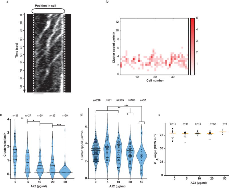
(a) Dynamic AglZ-YFP clusters in a non-motile cell observed by TIRFM. Kymograph representation of cluster movement captured every 0.5 s. Note that the clusters form at the cell pole and move directionally towards the opposite cell pole where they are dispersed. Scale bar = 2 μm. (b) Distribution of cluster speeds between and within cells. Note that clusters can move at different speeds in a cell and that the speed between cells generally varies between 2–4 μm.min-1. (c) Number of AglZ–YFP clusters per cell per minute in WT and A22 treated cells (2 technical replicates). (d) AglZ–YFP cluster speed in WT and A22 treated cells (2 technical replicates). Statistics as in (c). (e) Trajectory angles in WT and A22 treated cells (2 technical replicates). Statistics Wilcoxon tests. *: p<0.1; **: p<0.01; ***: p<0.001. Statistics as in (c).

Extended Data Figure 2. Myxococcus cells rotate along their long axis during motility.

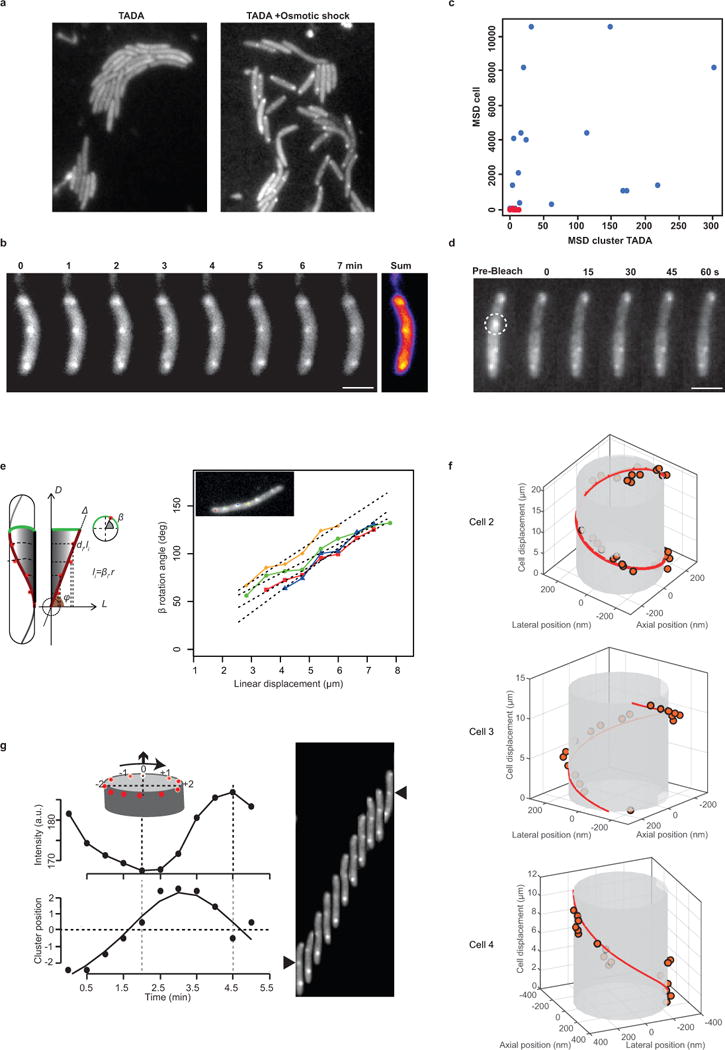
(a) TADA-bright clusters form in Myxococcus cells subjected to a brief osmotic shock. TADA is only incorporated in the Myxococcus cell envelope when the cells are subjected to NaCl treatment (see Methods).

(b–c) TADA-bright clusters are not dynamic in non-motile cells. TADA-bright cluster movements are not detectable in non-motile cells (c, red dots, n=14 ; 2 technical replicates) and only detectable in moving cells (c, blue dots, n=17 ; 2 technical replicates). MSD: Mean Square displacement. Scale bar = 2 μm.

(d) TADA-bright clusters are inert. Fluorescence Recovery After Photobleaching (FRAP) analysis reveals the absence of fluorescent molecule exchange in TADA-bright clusters (n=6 ; 1 technical experiment). Scale bar = 2 μm.

(e) TADA-bright cluster rotation reflects rotation of the cell during movement. A cell on which four TADA-bright clusters were tracked is shown. The radial velocity of each cluster calculated by projection of the 2D images on the model 3D cell cylinder (left panel, β angle) is plotted against the linear displacement of the cell. Each TADA cluster moved at the same radial speed and proportionally to the speed of the cell, indicating that TADA clusters are inert objects reporting on the rigid-body movement of the cell.

(f) 3D-trajectories of TADA-bright clusters reconstructed by astigmatism. We note that -in absence of astigmatism- the size of TADA clusters corresponds to the diffraction limit of light, and that they are circular (i.e. the size of the PSF is the same in perpendicular directions), making the astigmatic analysis of axial position possible.

(g) TADA-bright clusters rotate in the clockwise direction. Cluster intensity fluctuations and positions relative to the cell axis are shown over time (left) in a representative cell (right). The black arrow points to the analysed cluster. A representative cell is shown in the right panel which was isolated from others in the field with a black mask (n=10 ; 3 technical replicates).

Extended Data Figure 3. Analysis of AglZ-YFP, GltI-YFP and AglQ-mCherry in agl and glt mutant backgrounds.

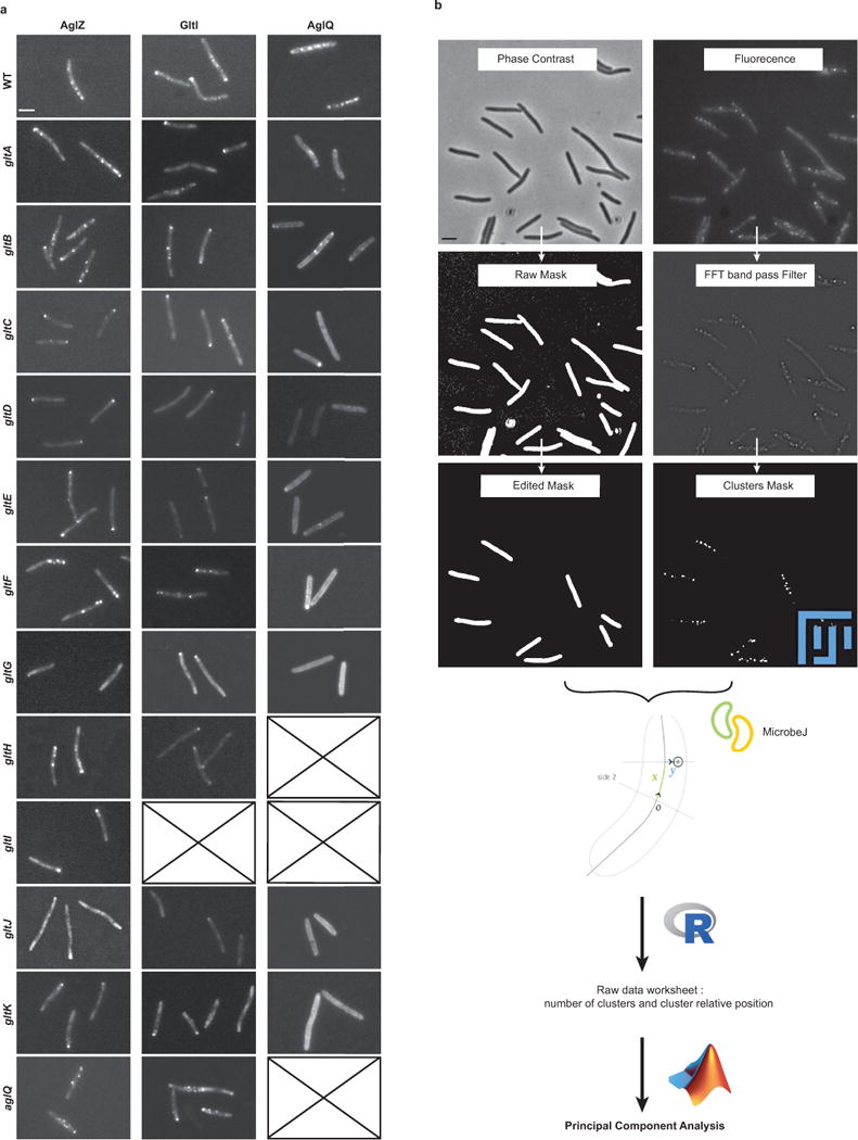
(a) Each fluorescent functional fusion was introduced in place of the WT gene in each genetic background shown. Typical examples are shown for each strain. Crossed boxes indicated genetic backgrounds that were not obtained for this study. Scale bar = 2 μm.

(b) Cluster detection and analysis chart. Phase contrast and fluorescence images were processed so as to respectively extract cell masks of isolated cells (compared edited mask to raw mask) and the position of fluorescence clusters following the application of a fluorescence bandpass filter. Note that the intensity of the fluorescence clusters was not exploited due to a lack of robustness and day-to-day fluctuations. The cluster coordinates were then defined relative to cell coordinates with the Microbe J plugin (http://www.indiana.edu/~microbej/) in Fiji, compiled in R sheets and further analyzed by Principal Component Analysis using custom-written code in Matlab.

Extended Data Figure 4. Principal Component Analysis (PCA) of AglZ-YFP, GltI-YFP and AglQ-mCherry in agl and glt mutant backgrounds.

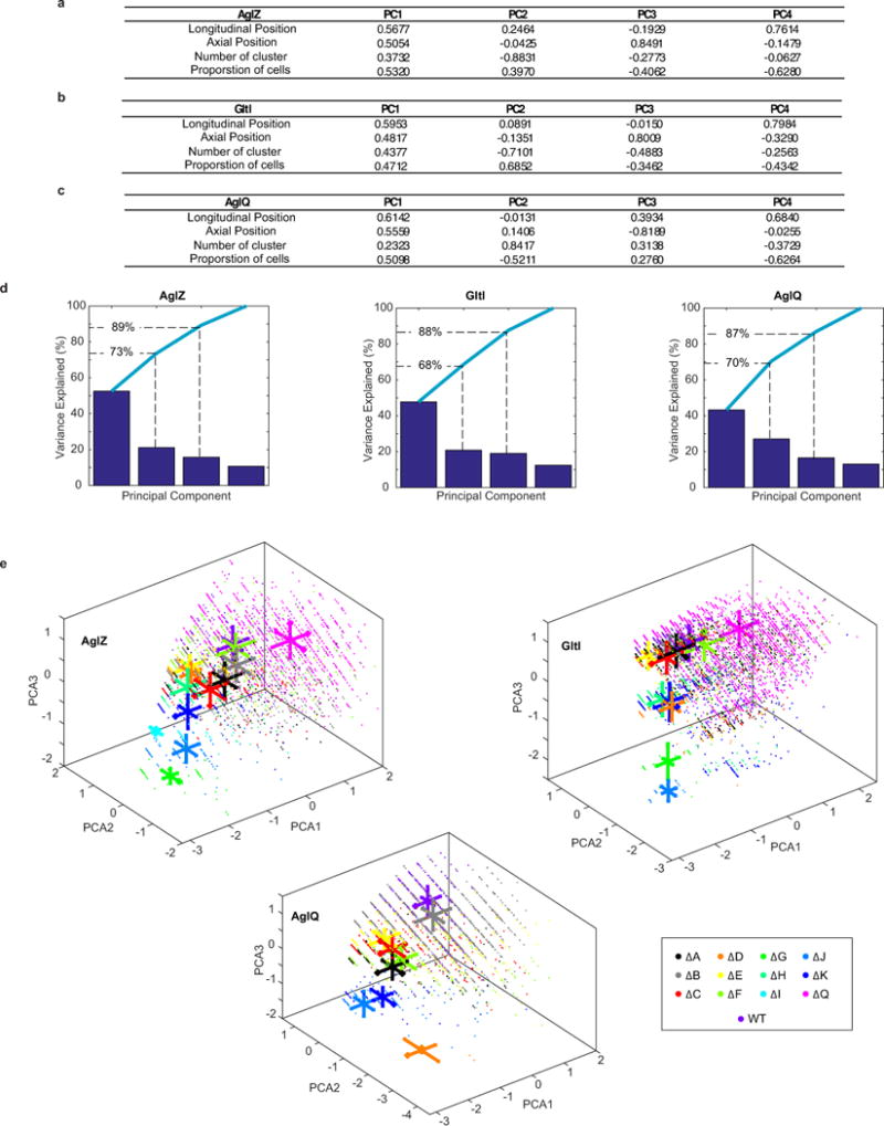
(a–c) Coefficients of the principal components (PC) for AglZ-YFP, GltI-YFP and AglQ-mCherry. PCs are the eigenvectors of the correlation matrix calculated from the four parameters indicated in the first column of the tables. Taken together, PCs form an orthogonal basis where the vectors are uncorrelated. PCs are sorted according to the amount of variability in the data they describe, PC1 having the largest effect (i.e. variance) and PC4 the least.

(d) Scree plots displaying the variance associated to each PC. Bar plot represents the variance associated to each PC for a given fusion (from left to right : AglZ-YFP, GltI-YFP and AglQ-mCherry). The cumulative variance is also plotted (light-blue line). Note that PC1-2 describe in average 70% of the total variance and PC1-3 more than 87%.

(e) Projection of the data in the space defined by the three first PCs. For each mutant, data are represented by a scatter plot of a specific colour (see inset for a detailed description of color code). For each direction and each mutant, the average and standard deviation of the data are symbolized by a single bold line : the center of the line represents the average and its length the standard deviation.

Extended Data Figure 5. Motility is propelled by cyclic interactions between the IM-localized motor and OM-localized adhesins of the motility complex.

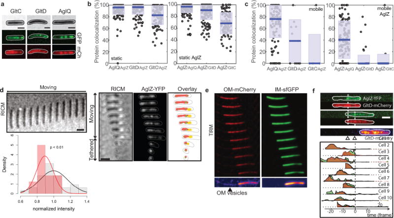
(a) Epifluorescence analysis of AglZ-YFP- AglQ/GltD/GltC-mCherry expressing representative cells. In each case, fluorescent functional fusions are expressed in place of the wild type gene. Note that while AglZ-YFP and AglQ-mCh clusters can be detected, GltC-mCh and GltD-mCh appear mostly diffuse around the cell envelope with these imaging conditions. 40 cells were imaged for AglZ-YFP/AglQ with 2 biological replicates; 232 cells were imaged for AglZ-YFP/AglD with 3 biological ; and 55 cells were imaged for AglZ-YFP/AglC with 3 biological. Scale bar = 2 μm.

(b) Protein co-localization in static clusters. For each cell analyzed, a percentage of colocalization is computed for proteins detected only in static clusters. Values range from 0 when no colocalization between the two proteins was detected in the cell to 100% when the two proteins were always detected together. For the left panel, the percentage of colocalization is represented for AglQ/GltD/GltI with respect to AglZ. Single data are represented by a scatter plot (o), the median colocalization value is symbolized by a blue line and the standard deviation by light-grey boxes. In average, 96% of AglQ clusters colocalized with AglZ (n=153 clusters ; 2 biological replicates), 96% for GltD (n=120 ; 7 biological replicates) and 83% for GltC (n=100 ; 3 biological replicates). Inversely, the right panel represents the percentage of colocalization of AglZ with respect to AglQ (97%, n=152 ; 2 biological replicates), GltD (91%, n=120 ; 7 biological replicates) and GltC (69%, n=100 ; 3 biological replicates), respectively.

(c) Protein co-localization in mobile clusters. Box-plots read as in (b) and describe the percentage of colocalization for proteins detected only in dynamic clusters. Left panel illustrates the colocalization of AglQ/GltD/GltI with respect to AglZ (76% n=106 ; 2 biological replicates, 39% n=11; 7 biological replicates and 0% n=4 respectively; 3biological replicates). Right panel describes the percentage of colocalization of AglZ with respect to AglQ (41%, n=125 ; 2 biological replicates), GltD (0%, n=72 ; 7 biological replicates) and GltC (0%, n=41 ; 3 biological replicates). Colocalization in dynamic clusters in only significative between AglZ and AglQ.

(d) AglZ-YFP clusters localize within adhesive contact zones. Left panel - RICM of a representative gliding cell (n=10 ; 2 biological replicates, 30 seconds time frames. Scale bar = 2 μm.) showing intimate connection with the chitosan-coated glass surface (dark zone). Right panel - Adhesions and AglZ-YFP cluster localization in detaching cells by RICM and combined epifluorescence microscopy (Time frames: 30 s. Scale bar = 2μm). The graph represents the distribution of RICM intensities at AglZ-YFP cluster positions (red line) compared to the average intensity along the whole cell body (black line). Data obtained for n=20 cells ; 2 biological replicates.

(e) Gliding Myxococcus cells deposit outer-membrane vesicles in their wake. TIRFM images of a motile cell expressing both an outer-membrane sfGFP and an inner membrane mCherry. OM vesicles are deposited suggesting that the cell is firmly adhered to the underlying surface. Shown is a representative cell (n=60 ; 12 technical replicates).

(f) GltD-mCherry, a periplasmic Glt protein, is not released by gliding cells at FA complexes Upper panel - TIRFM snapshots are shown for a representative cell expressing both GltD-mCherry (red) and AglZ-YFP (green). The position of the GltD clusters on the surface coincides with position of FA complexes (white asterisk). Time frames: 15s. Scale bar = 2μm. Lower panel - variation of intensity for GltD-mcherry (red) and AglZ-YFP (green) as a function of time before (negative time) and after (positive time) the cell moved away from the FA position, shown for n=10 cells (2 biological replicates).

Extended Data Figure 6. Image analysis for TIRFM experiments.

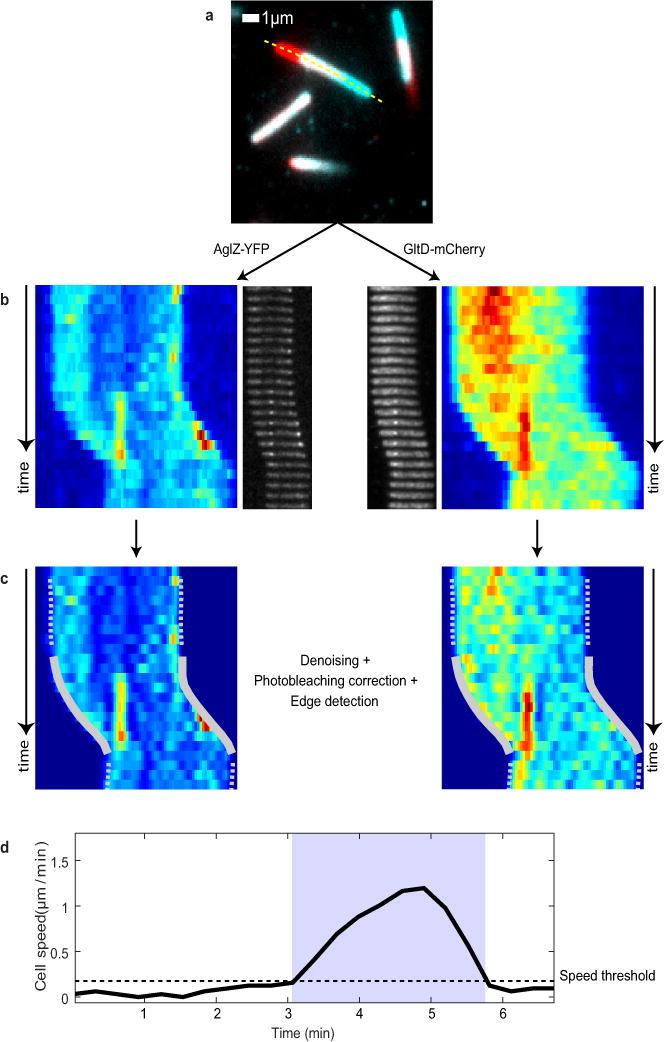
(a) Temporal RGB image computed from fluorescence images (mCherry for this example). Images were summed together and color coded from blue (first image) to red (last image). Immobile cells appeared uniformly white while moving cells showed colored extremities. Cell trajectory is represented by a yellow dotted line.

(b) For the two imaging channels (YFP and mCherry), a kymograph and a montage were calculated. Kymograph read from top (first image) to bottom (last image), each line representing the average fluorescent intensity computed along the cell trajectory. The montage showed for each acquisition an image of the cell after applying a straightening algorithm. Clusters of proteins (AglZ-YFP or AglQ/GltD/GltI-mCherry) appeared as bright spots at the center of the cell.

(c) Kymographs after applying a denoising algorithm. The cell outline was depicted by either a dotted white line when the cell was immobile or by a continuous white line when the cell was gliding on the surface.

(d) Cell speed as a function of acquisition time. For each cell, a threshold was defined that depended on the signal-to-noise ratio and the sample lateral stability during TIRFM acquisition. When the cell-speed was below this threshold (horizontal dotted line), the cell was considered immobile. Phases associated to cell movement are highlighted in blue.

Extended Data Figure 7. Colocalization estimation and correlation with cell movement.

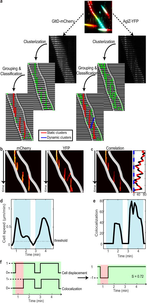
(a) Co-localization between YFP-tagged and mCherry-tagged proteins was calculated in three steps. For each channel (YFP and mCherry), a threshold was applied to the montage in order to detect protein clusters (clusterization). When the same cluster was observed in successive images, its localizations were stitched together manually and finally classified as either static (red) or dynamic/mobile (blue).

(b) For each channel, a protein-detection map was computed from the kymograph and the positions of the detected clusters. The cell outline was depicted by two white lines.

(c) The co-localization map was obtained by multiplying the two protein-detection maps. In the inset, the cumulative intensity associated to static (red) and dynamic (blue) clusters were plotted as a function of time.

(d) Cell-speed as a function of acquisition time. Blue boxes represent regions where cell speed is higher than the threshold.

(e) Cumulative co-localization intensity (static and dynamic) as a function of acquisition time. Blue boxes represent regions with high cell speed.

(f) Curves from (d) and (e) were binarized. For the cell-speed, the value was set to ‘0’ when the speed was below the threshold (immobilie cell) and to ‘1’ when it was above (gliding cell) (left panel). For the colocalization, the value was set to ‘1’ when co-localization was detected, ‘0’ otherwise (left panel). A correlation curve (right panel) was then computed by comparing the two curves. At each time-point, if the values of the two binarized curves were equal (1/1 or 0/0, green highlighted areas), the correlation was set to ‘1’. Else, it was set to ‘−1’ (red highlighted area). Finally, the correlation score was defined as the average of all the correlation values.

Extended Data Figure 8. Bionformatics analysis of AglQ/S and GltF.

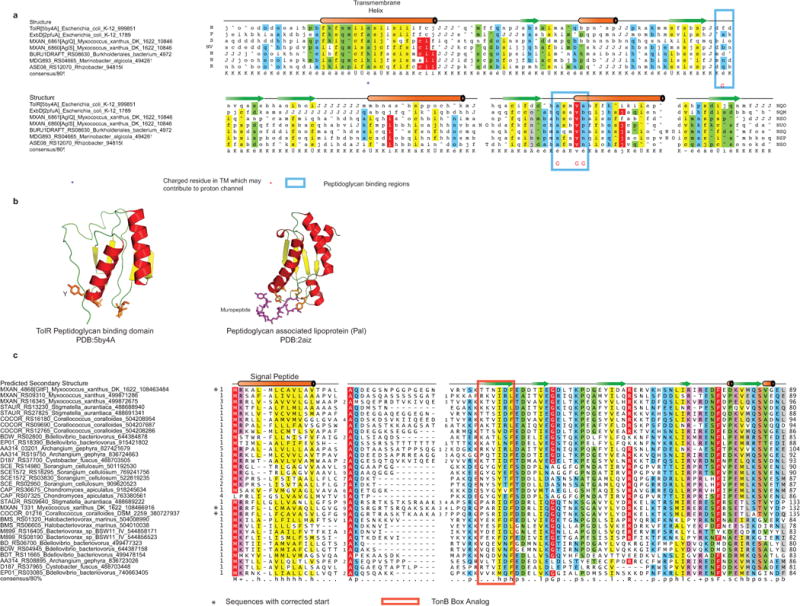
(a) AglQ and AglS carry a potential PG-binding site. Multiple Alignment of AglQ, AglS and their paralogs with TolR(5by4A) and ExbD (2pfuA). The gene name, organism name and GI are given. The structure is shown on top and the 80% consensus is shown below the alignment.

(b) Cartoon view of the structures are shown below with the residues known or predicted to bind peptidoglycan shown as sticks.

(c) The GltF family of proteins found in deltaproteobacteria. Multiple Alignment of the GltF family is shown and labeled using gene name, organism name and GI are given. The potential TonB box analog is indicated. The TonB box can be most generally defined as an extended region i.e. forming a beta strand-like structure that is not paired with other beta strands into a structural unit. The TonB-Box typically has two polar residues T/S and classically and acidic/amide residue. The GltF sequence profile analysis shows that GltF is related to the N-terminal region of certain OMP barrels that do contain a potential TonB-box like peptide.

Extended Data Figure 9. Bioinformatics analysis of the GltABH system.

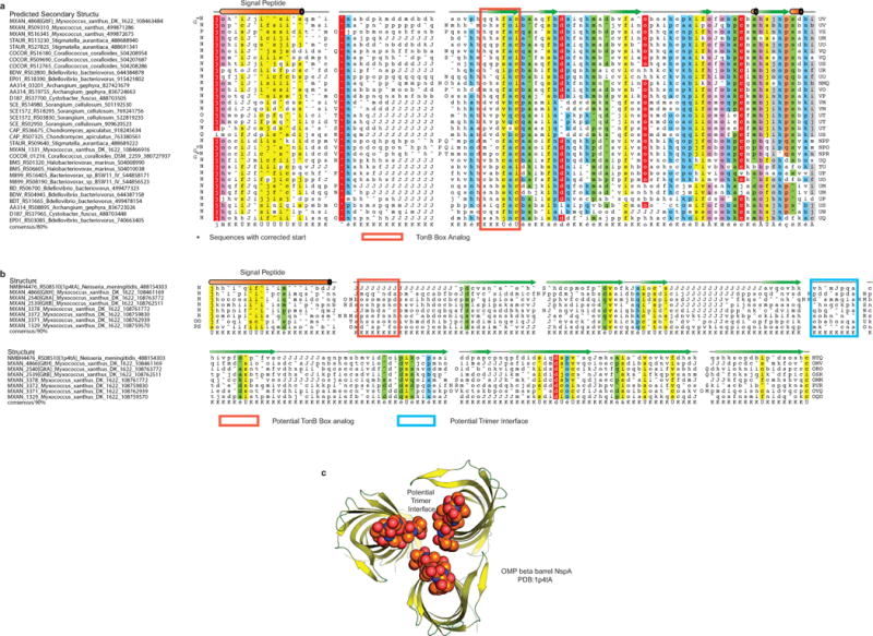
(a) Multiple alignment of the beta-barrel OMP proteins GltA, GltB and GltH and their paralogs with NspA (1p4tA). Note the presence of TonB-Box analogs in GltA and GltB but not in GltH.

(b) Cartoon view of the inferred trimer of beta barrels based on the NspA structure with the residues predicted to form a trimeric interaction interface shown in spheres.

References

- 1.Islam ST, Mignot T. The mysterious nature of bacterial surface (gliding) motility: A focal adhesion-based mechanism in Myxococcus xanthus. Semin Cell Dev Biol. 2015;46:143–154. doi: 10.1016/j.semcdb.2015.10.033. [DOI] [PubMed] [Google Scholar]
- 2.Luciano J, et al. Emergence and modular evolution of a novel motility machinery in bacteria. PLoS Genet. 2011;7:e1002268. doi: 10.1371/journal.pgen.1002268. [DOI] [PMC free article] [PubMed] [Google Scholar]
- 3.Sun M, Wartel M, Cascales E, Shaevitz JW, Mignot T. Motor-driven intracellular transport powers bacterial gliding motility. Proc Natl Acad Sci U S A. 2011;108:7559–7564. doi: 10.1073/pnas.1101101108. [DOI] [PMC free article] [PubMed] [Google Scholar]
- 4.Jakobczak B, Keilberg D, Wuichet K, Søgaard-Andersen L. Contact-and protein transfer-dependent stimulation of assembly of the gliding motility machinery in Myxococcus xanthus. PLoS Genet. 2015;11:e1005341. doi: 10.1371/journal.pgen.1005341. [DOI] [PMC free article] [PubMed] [Google Scholar]
- 5.Nan B, et al. Myxobacteria gliding motility requires cytoskeleton rotation powered by proton motive force. Proc Natl Acad Sci U S A. 2011;108:2498–2503. doi: 10.1073/pnas.1018556108. [DOI] [PMC free article] [PubMed] [Google Scholar]
- 6.Balagam R, et al. Myxococcus xanthus gliding motors are elastically coupled to the substrate as predicted by the focal adhesion model of gliding motility. PLoS Comput Biol. 2014;10:e1003619. doi: 10.1371/journal.pcbi.1003619. [DOI] [PMC free article] [PubMed] [Google Scholar]
- 7.Treuner-Lange A, et al. The small G-protein MglA connects to the MreB actin cytoskeleton at bacterial focal adhesions. J Cell Biol. 2015;210:243–256. doi: 10.1083/jcb.201412047. [DOI] [PMC free article] [PubMed] [Google Scholar]
- 8.Nan B, et al. Flagella stator homologs function as motors for myxobacterial gliding motility by moving in helical trajectories. Proc Natl Acad Sci U S A. 2013;110:E1508–13. doi: 10.1073/pnas.1219982110. [DOI] [PMC free article] [PubMed] [Google Scholar]
- 9.Kaiser D, Warrick H. Transmission of a signal that synchronizes cell movements in swarms of Myxococcus xanthus. Proc Natl Acad Sci U S A. 2014;111:13105–13110. doi: 10.1073/pnas.1411925111. [DOI] [PMC free article] [PubMed] [Google Scholar]
- 10.Bean GJ, et al. A22 disrupts the bacterial actin cytoskeleton by directly binding and inducing a low-affinity state in MreB. Biochemistry. 2009;48:4852–4857. doi: 10.1021/bi900014d. [DOI] [PMC free article] [PubMed] [Google Scholar]
- 11.Huang B, Wang W, Bates M, Zhuang X. Three-dimensional super-resolution imaging by stochastic optical reconstruction microscopy. Science. 2008;319:810–813. doi: 10.1126/science.1153529. [DOI] [PMC free article] [PubMed] [Google Scholar]
- 12.Wojdyla JA, et al. Structure and function of the Escherichia coli Tol-Pal stator protein TolR. J Biol Chem. 2015;290:26675–26687. doi: 10.1074/jbc.M115.671586. [DOI] [PMC free article] [PubMed] [Google Scholar]
- 13.Gresock MG, Kastead KA, Postle K. From Homodimer to Heterodimer and Back: Elucidating the TonB Energy Transduction Cycle. J Bacteriol. 2015;197:3433–3445. doi: 10.1128/JB.00484-15. [DOI] [PMC free article] [PubMed] [Google Scholar]
- 14.Wartel M, et al. A versatile class of cell surface directional motors gives rise to gliding motility and sporulation in Myxococcus xanthus. PLoS Biol. 2013;11:e1001728. doi: 10.1371/journal.pbio.1001728. [DOI] [PMC free article] [PubMed] [Google Scholar]
- 15.Bui NK, et al. The peptidoglycan sacculus of Myxococcus xanthus has unusual structural features and is degraded during glycerol-induced myxospore development. J Bacteriol. 2009;191:494–505. doi: 10.1128/JB.00608-08. [DOI] [PMC free article] [PubMed] [Google Scholar]
- 16.Cascales E, Gavioli M, Sturgis JN, Lloubès R. Proton motive force drives the interaction of the inner membrane TolA and outer membrane pal proteins in Escherichia coli. Mol Microbiol. 2000;38:904–915. doi: 10.1046/j.1365-2958.2000.02190.x. [DOI] [PubMed] [Google Scholar]
- 17.Wang S, Furchtgott L, Huang KC, Shaevitz JW. Helical insertion of peptidoglycan produces chiral ordering of the bacterial cell wall. Proc Natl Acad Sci U S A. 2012;109:E595–604. doi: 10.1073/pnas.1117132109. [DOI] [PMC free article] [PubMed] [Google Scholar]
- 18.Ejigiri I, et al. Shedding of TRAP by a rhomboid protease from the malaria sporozoite surface is essential for gliding motility and sporozoite infectivity. PLoS Pathog. 2012;8:e1002725. doi: 10.1371/journal.ppat.1002725. [DOI] [PMC free article] [PubMed] [Google Scholar]
- 19.den Blaauwen T, de Pedro MA, Nguyen-Distèche M, Ayala JA. Morphogenesis of rod-shaped sacculi. FEMS Microbiol Rev. 2008;32:321–344. doi: 10.1111/j.1574-6976.2007.00090.x. [DOI] [PubMed] [Google Scholar]
- 20.Nan B, Mauriello EMF, Sun IH, Wong A, Zusman DR. A multi-protein complex from Myxococcus xanthus required for bacterial gliding motility. Mol Microbiol. 2010;76:1539–1554. doi: 10.1111/j.1365-2958.2010.07184.x. [DOI] [PMC free article] [PubMed] [Google Scholar]
Methods References
- 1.Bustamante VH, Martínez-Flores I, Vlamakis HC, Zusman DR. Analysis of the Frz signal transduction system of Myxococcus xanthus shows the importance of the conserved C-terminal region of the cytoplasmic chemoreceptor FrzCD in sensing signals. Mol Microbiol. 2004;53:1501–1513. doi: 10.1111/j.1365-2958.2004.04221.x. [DOI] [PubMed] [Google Scholar]
- 2.Wartel M, et al. A versatile class of cell surface directional motors gives rise to gliding motility and sporulation in Myxococcus xanthus. PLoS Biol. 2013;11:e1001728. doi: 10.1371/journal.pbio.1001728. [DOI] [PMC free article] [PubMed] [Google Scholar]
- 3.Ducret A, Theodoly O, Mignot T. Single cell microfluidic studies of bacterial motility. Methods Mol Biol. 2013;966:97–107. doi: 10.1007/978-1-62703-245-2_6. [DOI] [PubMed] [Google Scholar]
- 4.Altschul SF, et al. Gapped BLAST and PSI-BLAST: a new generation of protein database search programs. Nucleic Acids Res. 1997;25:3389–3402. doi: 10.1093/nar/25.17.3389. [DOI] [PMC free article] [PubMed] [Google Scholar]
- 5.Johnson LS, Eddy SR, Portugaly E. Hidden Markov model speed heuristic and iterative HMM search procedure. BMC Bioinformatics. 2010;11:431. doi: 10.1186/1471-2105-11-431. [DOI] [PMC free article] [PubMed] [Google Scholar]
- 6.Söding J, Biegert A, Lupas AN. The HHpred interactive server for protein homology detection and structure prediction. Nucleic Acids Res. 2005;33:W244–8. doi: 10.1093/nar/gki408. [DOI] [PMC free article] [PubMed] [Google Scholar]
- 7.Holm L, Kääriäinen S, Rosenström P, Schenkel A. Searching protein structure databases with DaliLite v.3. Bioinformatics. 2008;24:2780–2781. doi: 10.1093/bioinformatics/btn507. [DOI] [PMC free article] [PubMed] [Google Scholar]
- 8.Lassmann T, Frings O, Sonnhammer ELL. Kalign2: high-performance multiple alignment of protein and nucleotide sequences allowing external features. Nucleic Acids Res. 2009;37:858–865. doi: 10.1093/nar/gkn1006. [DOI] [PMC free article] [PubMed] [Google Scholar]
- 9.Pei J, Sadreyev R, Grishin NV. PCMA: fast and accurate multiple sequence alignment based on profile consistency. Bioinformatics. 2003;19:427–428. doi: 10.1093/bioinformatics/btg008. [DOI] [PubMed] [Google Scholar]
- 10.Drozdetskiy A, Cole C, Procter J, Barton GJ. JPred4: a protein secondary structure prediction server. Nucleic Acids Res. 2015;43:W389–94. doi: 10.1093/nar/gkv332. [DOI] [PMC free article] [PubMed] [Google Scholar]
- 11.Finn RD, et al. Pfam: the protein families database. Nucleic Acids Res. 2014;42:D222–30. doi: 10.1093/nar/gkt1223. [DOI] [PMC free article] [PubMed] [Google Scholar]
- 12.Krogh A, Larsson B, von Heijne G, Sonnhammer EL. Predicting transmembrane protein topology with a hidden Markov model: application to complete genomes. J Mol Biol. 2001;305:567–580. doi: 10.1006/jmbi.2000.4315. [DOI] [PubMed] [Google Scholar]
- 13.Käll L, Krogh A, Sonnhammer ELL. A combined transmembrane topology and signal peptide prediction method. J Mol Biol. 2004;338:1027–1036. doi: 10.1016/j.jmb.2004.03.016. [DOI] [PubMed] [Google Scholar]
- 14.Marbouty M, et al. Condensin- and Replication-Mediated Bacterial Chromosome Folding and Origin Condensation Revealed by Hi-C and Super-resolution Imaging. Mol Cell. 2015;59:588–602. doi: 10.1016/j.molcel.2015.07.020. [DOI] [PubMed] [Google Scholar]
- 15.Ducret A, Valignat MP, Mouhamar F, Mignot T, Theodoly O. Wet-surface-enhanced ellipsometric contrast microscopy identifies slime as a major adhesion factor during bacterial surface motility. Proc Natl Acad Sci U S A. 2012;109:10036–10041. doi: 10.1073/pnas.1120979109. [DOI] [PMC free article] [PubMed] [Google Scholar]
- 16.Schindelin J, et al. Fiji: an open-source platform for biological-image analysis. Nat Methods. 2012;9:676–682. doi: 10.1038/nmeth.2019. [DOI] [PMC free article] [PubMed] [Google Scholar]
- 17.Arigovindan M, et al. High-resolution restoration of 3D structures from widefield images with extreme low signal-to-noise-ratio. Proc Natl Acad Sci U S A. 2013;110:17344–17349. doi: 10.1073/pnas.1315675110. [DOI] [PMC free article] [PubMed] [Google Scholar]
- 18.Marques O. Practical image and video processing using MATLAB. John Wiley & Sons; 2011. [Google Scholar]
- 19.Wolter S, et al. rapidSTORM: accurate, fast open-source software for localization microscopy. Nat Methods. 2012;9:1040–1041. doi: 10.1038/nmeth.2224. [DOI] [PubMed] [Google Scholar]
Associated Data
This section collects any data citations, data availability statements, or supplementary materials included in this article.
Supplementary Materials
Data Availability Statement