Nonuniform Moving Boundary Method for Computational Fluid Dynamics Simulation of Intrathecal Cerebrospinal Flow Distribution in a Cynomolgus Monkey

Abstract

A detailed quantification and understanding of cerebrospinal fluid (CSF) dynamics may improve detection and treatment of central nervous system (CNS) diseases and help optimize CSF system-based delivery of CNS therapeutics. This study presents a computational fluid dynamics (CFD) model that utilizes a nonuniform moving boundary approach to accurately reproduce the nonuniform distribution of CSF flow along the spinal subarachnoid space (SAS) of a single cynomolgus monkey. A magnetic resonance imaging (MRI) protocol was developed and applied to quantify subject-specific CSF space geometry and flow and define the CFD domain and boundary conditions. An algorithm was implemented to reproduce the axial distribution of unsteady CSF flow by nonuniform deformation of the dura surface. Results showed that maximum difference between the MRI measurements and CFD simulation of CSF flow rates was <3.6%. CSF flow along the entire spine was laminar with a peak Reynolds number of ∼150 and average Womersley number of ∼5.4. Maximum CSF flow rate was present at the C4-C5 vertebral level. Deformation of the dura ranged up to a maximum of 134 μm. Geometric analysis indicated that total spinal CSF space volume was ∼8.7 ml. Average hydraulic diameter, wetted perimeter, and SAS area were 2.9 mm, 37.3 mm and 27.24 mm², respectively. CSF pulse wave velocity (PWV) along the spine was quantified to be 1.2 m/s.

Introduction

Cerebrospinal fluid (CSF) plays a vital role in the immunological support, structural protection, and metabolic homeostasis of the CNS. A detailed understanding of CSF dynamics may improve treatment of several CNS diseases and help to optimize CSF system-based CNS therapeutics. The importance of CSF dynamics has been investigated in several CNS diseases that include syringomyelia [1], Alzheimer's disease [2], Chiari malformation [3], and hydrocephalus [4]. Recent studies have examined the possible role of CSF as a conduit for distribution of therapeutic molecules to neuronal and glial cells of CNS tissues [5,6]. Intrathecal-based CNS therapeutics for treatment of devastating CNS disorders such as Alzheimer's, amyotrophic lateral sclerosis, Parkinson's, and autism are under investigation. Researchers found that brain tissue is rapidly “washed out” with CSF during sleep in a mouse model [7]. Tracer studies showed that solutes within the CSF are transported into and out of the brain tissue via a leptomeningeal or perivascular pathway [8]. While many studies have shown increasing importance of the role of CSF in CNS system homeostasis, there is a paucity of information on CSF biofluid mechanics.

Cerebrospinal fluid-based brain therapeutics are gaining interest because they allow direct pharmaceutical targeting of the CNS that can help minimize some side effects associated with conventional oral and intravenous-based pharmacotherapies and allows delivery of larger molecule sizes to the CNS that may not normally be able to cross the blood–brain barrier. The CSF is a promising route with many potentially important roles for CNS therapeutics such as: (a) direct delivery of large drug molecules to the CNS tissue that is not possible via blood injection due to the blood brain barrier, (b) CSF filtration, termed neuropheresis, to remove unwanted toxins in diseases such as meningitis, and (c) CSF cooling, termed CSF hypothermia, to slow down traumatic brain and spinal cord (SC) injury following severe accidents. However, while CNS therapeutics have a great deal of potential, they require expensive and restricted nonhuman primate (NHP) studies to reach clinical use. This expense makes detailed testing and optimization of brain therapeutic systems and medications difficult.

There is a need to develop a CSF hydrodynamic simulator (flow model) with a realistic geometry and CSF flow distribution. Such a simulator will allow testing and optimization of CNS therapeutics. Since these therapies often require testing on NHPs, our approach was to develop a subject-specific numerical model of CSF hydrodynamics in a cynomolgus monkey, a commonly used species for these studies. The focus of this numerical model was accurate representation of the spinal SAS CSF flow rate and waveform distribution as intrathecal infusion is primarily conducted within the spine. Comparison of CSF dynamics within the numerical model and MRI flow measurements were made to understand its hydrodynamic similarity to in vivo.

Materials and Methods

Measured Data

Ethics Statement.

This study was submitted to and approved by the local governing Institutional Animal Care and Use Committee (IACUC). This study did not unnecessarily duplicate previous experiments, and alternatives to the use of live animals were considered. Procedures used in this study were designed with the consideration of the well-being of the animals.

Animal Selection.

A healthy 4 year old adult male cynomolgus monkey (Macaca fascicularis, origin Mauritius) from Charles River Research Models, Houston, TX with a weight of 4.39 kg was selected for the study. This animal was purpose-bred and experimentally naïve.

Pre-MRI NHP Preparation.

The NHP was positioned in the scanner in the supine orientation with natural breathing (no mechanical ventilation). During each scan, heart rate (HR) and respiration was monitored with ∼1 l/min of oxygen and 1–3% isoflurane anesthetic was administered via oral mask for sedation and intubation for the duration of the scanning procedures.

MRI Scan Protocols.

MRI measurements were collected at Northern Biomedical Research on a Philips 3T scanner (achieva, software V2.6.3.7, Best, The Netherlands). This NHP did not have prior administration of intrathecal drugs and/or catheter systems in the spine. Total scan time to quantify SAS geometry and flow, not including pre-MRI NHP preparation, was 1 h and 21 min.

Phase-Contrast MRI Protocol for CSF Flow Detection.

Phase-contrast MRI measurements were collected with retrospective electrocardiogram (ECG) gating and 24 heart phases were reconstructed over the cardiac cycle. In-plane resolution was reconstructed at 0.45 × 0.45 mm and slice thickness was 5.0 mm. Slice location for each scan was oriented perpendicular to the CSF flow direction with slice planes intersecting vertebral disks. These locations included the foramen magnum (FM) and vertebral disks located between the C2-C3, T4-T5, T10-T11 and L2-L3 vertebral levels (Fig. 1(a)). Velocity encoding value was 5 cm/s at the FM and L2-L3, and 10 cm/s at all other locations.

Fig. 1.

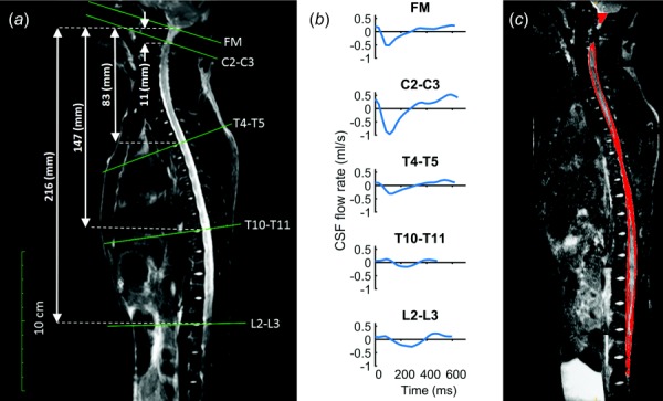
(a) T2-weighted MR image of the entire spine for the cynomolgus monkey analyzed. Axial location and slice orientation (solid lines) of the phase-contrast MRI scans obtained in the study. Slice axial distance from foramen magnum indicated by dotted lines. (b) The CSF flow rate based on in vivo PCMRI measurement at FM, C2-C3, T4-T5, T10-T11, and L2-L3. (c) Sagittal view of the SAS segmentation based on T2-weighted MRI.

MRI CSF Space Geometry Protocol.

A stack of 720 axial images were acquired using a volumetric isotropic T2w acquisition (VISTA) for complete coverage of the spinal SAS geometry (Fig. 1(a)). Scan time was 55 min with parameters indicated in Table 1. The anatomical region scanned was ∼31 cm in length and included the entire spinal SAS extending caudally to the filum terminale. Images had a 0.5 mm slice spacing and 0.38 mm isotropic in-plane resolution.

Table 1.

Anatomic and CSF flow MRI scan protocol parameters

Parameter	Anatomic (T2-VISTA)	CSF flow (phase-contrast MRI)
Acquisition contrast	T2	Flow encoded
Acquisition type	3D	2D
Slice thickness	1 mm	5
Slice spacing	0.5 mm	N/A
Pixel bandwidth	481	192
Pulse sequence	TSE	TFE
Transmit coil	15 ch. sense spine coil	15 ch. sense spine coil
Duration	55 min	4 min each (20 min total)
Number of slices	660	N/A
Image matrix	864 × 864	224 × 224
In-plane resolution	0.375 mm isotropic	0.446 mm isotropic
TR	2000	11.293
TE	120	6.774
Cardiac phases	N/A	24
R–R interval	N/A	482–644 ms
Encoding direction	N/A	Thru-plane
Plane orientation	Axial	Axial
Trigger	N/A	Retrospective ECG
Velocity encoding	N/A	5 cm/s at FM and L2-L310 cm/s at C2-C3, T4-T5, T10-T11

CSF Flow Quantification.

CSF flow was quantified for each of the axial locations shown in Fig. 1(b). As detailed in our previous studies [9,10], the CSF flow waveform, $Q_{(t)}$, was computed within matlab based on integration of the pixel velocities with $Q(t)=\sum A_{\text{pixel}}[V_{\text{pixel}}(t)]$, where A_pixel is the area of one MRI pixel, V_pixel is the velocity for the corresponding pixel, and $Q_{(t)}$ is the summation of the flow for each pixel of interest as in our previous studies.

MRI Geometry Postprocessing.

The high-resolution T2-weighted anatomic MRI images were semi-automatically segmented using the free open-source itk-snap software (Version 3.0.0, University of Pennsylvania, Philadelphia, PA). Details on the segmentation procedure are provided in our previous work [11]. SC nerve roots and denticulate ligaments were not included in the model as they were not possible to accurately quantify at the acquired MRI resolution. Individual SC nerves were quantified at the filum terminale. The final segmentation (Fig. 1(c)) was exported in stereolithography format (Fig. 2(a)). The initial geometry of the numerical model was based on the time-averaged geometry measured over the MRI acquisition period.

Fig. 2.

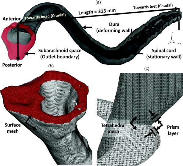
(a) Three-dimensional CFD model of the SAS, (b) zoom of the upper cervical spine mesh showing the model inlet (top), and (c) volumetric mesh visualization in the axial and sagittal planes within the cervical SAS

Flow Model.

Our overall flow model approach was to solve for the CSF flow field within the spinal SAS using CFD with a specified moving boundary motion based on the in vivo MRI measurements. The volume flow rate of the incompressible CSF flow along the spine was purely determined by the mass/volume conservation. Results were verified based on numerical independence studies, quantified in terms of geometry and hydrodynamics, and validated based on comparison of the in vivo measurements.

Nonuniform Mesh Deformation to Reproduce CSF Flow Along Spine.

The phase-contrast MRI measurements showed a complex nonuniform distribution of CSF flow along the spine. Thus, to reproduce the nonuniform flow, a nonuniform deformation of the computational mesh was implemented at each time step by a user-defined function (UDF) applied within ansys fluent (ANSYS^® Academic Research, Release 17.2). A spring-based smoothing algorithm was applied to the mesh based on the calculated deformation within each section, as described in the following steps (Flow chart with steps 1–7 indicated in Fig. 3(a)):

Fig. 3.

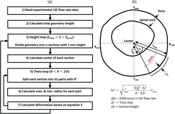
(a) Dynamic mesh motion flow chart used for the CFD simulation. Recursive arrows indicate repetition of steps. (b) A 2D axial cross section with relevant variables and key equation used to compute radial deformation of the dura.

Step 1. In vivo CSF flow rates along the spine were measured at five distinct locations (Fig. 1(b)). To generate a smooth CSF flow distribution along the spine within 1 mm sections, these five distinct flow rates were spatial-temporal filtered in matlab using the 2D “fit” function with fittype = “spline” configuration. Some HR variability was present between the phase-contrast magnetic resonance imaging (PCMRI) scans. Thus, the diastolic portion of the CSF flow waveforms with a shortened cardiac cycle was extended using methods previously developed by Schmidt-Daners and coworkers [12]. Maximum waveform extension was 180 ms at T10-T11. The smooth CSF flow distribution along the spine was then read into the mesh deformation algorithm (Fig. 3(a)).

Step 2. Maximum and minimum geometry height in the caudocranial direction (Z_max and Z_min) was calculated. Total model length was calculated as the difference of these values $(\text{Length}=Z_{\text{max}}-Z_{\min })$.

Step 3. To apply the nonuniform deformation on each spine node, the entire geometry was divided into “n” sections with 1 mm height (315 total sections with $\Delta h=1\hspace{0.17em}\text{mm}$). Total model length was 315 mm.

Step 4. The center of each section was defined based on the maximum and minimum location along the X- and Y-axis based on the below equation

$$\begin{array}{c}{X}_C=\frac{X_{\max }-X_{\min }}{2}+X_{\min }\\ Y_C=\frac{Y_{\max }-Y_{\min }}{2}+Y_{\min }\end{array}$$ (1)

where subscripts max, min, and C denote maximum, minimum, and center of each section, respectively (see Fig. 3(b) for diagram).

Step 5. To identify the dura and SC location, each section was divided into 32 parts each containing 11.25 deg (10,080 total parts for entire model). Further calculations of mesh deformation were repeated for each part.

Step 6. Our approach was to move the dura location and maintain the SC in a fixed position (SC compressibility is likely small). A limitation value (see Fig. 3(b)) was calculated based on the maximum and minimum radius of each part using the below equation

$$\mathrm{Limit}=r_{\min }+\frac{r_{\max }-r_{\min }}{2}$$ (2)

Each point with a greater radius than the limit value was allowed to move during the simulation and all others remained fixed in location.

Step 7. The time-course radial displacement for each node within each part was calculated based on the difference in CSF flow rate across each section ($\Delta Q$). This variation was assumed equal to the volume change of each section at each time step ($\Delta V=\Delta Q\cdot \Delta t$). Where $\Delta t$ denotes solver time-step size. Under the assumption of zero dura and SC axial motion along the Z-axis, deformation was only calculated within the XY-plane (Fig. 3(b)). Due to the relatively small angle within each part (11.25 deg), the outer boundary of each part (dura) was assumed as a circular arc. Thus, radial displacement of each node on the dura surface for each part, $\Delta r$, was computed based on area variation within that pseudo-circular part, where $\Delta A=\Delta V/\Delta h$, using the below equation

$$\Delta r=\sqrt{r_{\max }^2-\Delta A}-r_{\max }=\sqrt{r_{\max }^2-\frac{\Delta Q\cdot \Delta t}{\pi \cdot \Delta h}}-r_{\max }$$ (3)

Numerical Solver Settings.

The computational domain with nonuniform unstructured grid (Fig. 2(b)) was generated within ansys icem cfd software and consisted of approximately 11.2 million tetrahedral elements (Fig. 2(c)). The commercial finite volume CFD solver ansy fluent was used to solve the continuity (Eq. (4)) and Navier–Stokes (Eq. (5)) equations numerically using the finite volume method

$$\nabla \cdot (\rho u)=0$$ (4)

$$\rho (\frac{\partial u}{\partial t}+u\cdot \nabla u)=-\nabla P+\mu {\nabla }^{2}u$$ (5)

where ρ is the density, μ is the dynamic viscosity, and u and $p$ describe the velocity and pressure fields, respectively.

The laminar viscous model was used to simulate laminar incompressible Newtonian flow. CSF hydrodynamic characteristics were considered to be equivalent with water at body temperature [13,14] (density of ρ = 993.3 kg/m³ and dynamic viscosity of μ = 0.6913 mPa·s). A no-slip boundary condition was imposed at the walls. A pressure-outlet boundary condition with 0 Pa gauge pressure was defined at the model cranial opening. Flow at the model cranial opening was produced based on the nonuniform deformation of the model wall. The model was terminated at the caudal end and was only open at the cranial end (Fig. 2). Thus, it was unnecessary to prescribe an inlet velocity boundary condition. Deformation of the outlet boundary was set as a faceted wall. Second-order upwind numerical scheme was used for both momentum and pressure gradient solver settings. The utilized transient formulation was second-order implicit with default values for under-relaxation factors. The convergence criteria for continuity and velocity were set to 1 × 10⁻⁸. CFD simulation for each cycle required ∼14 h to complete in parallel mode with 141 GB RAM and 30 processors at a clock speed of 2.3 GHz. Total simulation time was 28 h for the two cycles simulated. Results are presented for the second cycle only.

Verification Studies.

To verify our numerical results, independence studies were carried out to determine the effect of cycle, mesh size, and time-step size on velocity results for a 6 cm model length located within the thoracic spine (Fig. 4(a), Table 2). Our focus was velocity since velocity was the parameter measured by the MRI measurements used to define the numerical model. A baseline simulation was conducted for a coarse tetrahedral mesh with wall prism layers containing a total of 0.6 million cells. Subsequent “medium” and “fine” simulations were carried out with mesh size and prism layer length halved for each case. Results were assessed at three axial slice locations separated by a 2 cm distance. For each slice, z-direction velocities, V_w, were quantified using a rake containing n = 1000 points along a straight line (Fig. 4(b)). Maximum error between each case was calculated at peak systolic flow using the following equation:

Fig. 4.

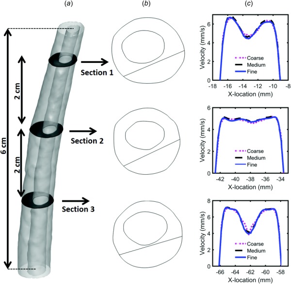
(a) Three-dimensional geometry of the independence study and axial plane positions, (b) line location along each plane, and (c) peak systolic w-velocity component visualized along each line for the three grids (coarse, medium, and fine)

Table 2.

Verification of results by numerical independence studies—values show the maximum relative error for velocity in the z-direction for the three axial planes analyzed (Fig. 4)

Independence study	Parameter to study	Constant parameters	Maximum error (%)
Grid size	MS = 0.5 mm, GS = 0.6 M	TS = CT/66	10.76
	PS = 0.05 mm, PN = 3
	MS = 0.25 mm, GS = 1.2 M	CN = 2	4.77
	PS = 0.025 mm PN = 5
	MS = 0.125 mm, GS = 7.5 M
PS = 0.0125 mm, PN = 8
Time step size	CT/33	GS = 1.2 M	10.34
	CT/66	CN = 2	2.06
CT/132
Period number	1	GS = 1.2 M	40.0
	2	TS = CT/66	1.59
3

Note: GS, grid size; PS, prism size; PN, prism number; MS, mesh size; CN, cycle number; M, million cells; CT, cycle time in seconds; TS, time step size.

$$\text{error}=\max \left(\left|\frac{V_{\text{wfine}(\text{tsys},n)}-V_{\text{wmedium}(\text{tsys},n)}}{\text{mean}\left(V_{\text{wfine}(\text{tysy},n)}\right)}\right|\right)\times 100$$ (6)

Maximum error for the medium versus fine grid was 4.7% and coarse versus medium grid was 10.76%. Thus, subsequent independence studies were carried out with the medium grid. Three time-step sizes were investigated through three flow cycles. Unsteady velocity was monitored at three different points within each of the slice locations and used to compute error (i.e., $V_{\text{wfine}(\text{tsys},n)}=V_{\text{wfine}(t)}$ in Eq. (4)). A time-step size of 0.01 s was selected for future studies having a maximum error of 2.1%. Similarly, cycle independence results for unsteady velocity showed that velocity variation after the first cycle was negligible (∼1.5%). Thus, results for the final CFD study were analyzed based on the second cycle with a medium grid and time-step size of 0.01 s.

Geometric Quantification.

Based on the 3D reconstruction and meshing, the following geometric parameters were calculated along the spine at 1 mm intervals similar to our previous studies [9]. Cross-sectional area of SAS, $A_{\mathit{c}\mathit{s}}=A_d-A_c$, was determined based on cross-sectional area of the SC, A_c, and dura, A_d. Hydraulic diameter for internal flow within a tube, $D_H=4A_{\mathit{c}\mathit{s}}/P_{\mathit{c}\mathit{s}}$, was determined based on the cross-sectional area and wetted perimeter, $P_{\mathit{c}\mathit{s}}=P_d+P_c$. Wetted perimeter was computed as the sum of the SC, P_c, and dura, P_d, perimeter. Each of these parameters was calculated within an UDF compiled in ansys fluent after the computational mesh was formed. The MRI-based time-averaged geometry, at baseline or zero deformation, was used to compute the above parameters.

Hydrodynamic Quantification.

The hydrodynamic environment at 1 mm slice intervals along the entire spine was assessed by Reynolds number based on peak flow rate, Re = ((Q_sysD_H)/(νA_cs)), and Womersley number based on hydraulic diameter. In this equation, Q_sys is the temporal maximum of the local flow at each axial location along the spine obtained by interpolation from the experimental data and ν is the kinematic viscosity of the fluid. CSF was assumed to have a viscosity of water at body temperature. Reynolds number at peak systole, or the ratio of steady inertial forces to viscous forces, was utilized as an indicator of the presence of laminar flow $(\mathrm{Re}<2300)$ along the spine. It should be noted that this formulation of Reynolds number is only an indicator of laminar flow for flow within a straight circular pipe. We provide this number for comparison to many previous studies in the field that have used it as an indicator of the flow type [11]. Womersley number, $\alpha =(D_h/2)\sqrt{\omega /\nu }$, was computed where ω is the angular velocity of the volume flow waveform with $\omega =2\pi /T$ and ν is the kinematic viscosity of CSF ($\nu =\mu /\rho$). Womersley number was used to quantify the ratio of unsteady inertial forces to viscous forces, which was found to be large for SAS CSF flow relative to viscous forces by Loth et al. [15]. A Womersley number greater than 5 indicates transition from parabolic to “m-shaped” peak-systolic velocity profiles for oscillatory flows [16]. CSF PWV was quantified as an indicator of CSF space stiffness. PWV was quantified based on the timing of peak systolic CSF flow rate along the spine using a method similar to Kalata et al. [17]. A linear fit was computed based on the peak systolic flow rate arrival time with the slope being equivalent to the PWV.

Validation of Numerical Simulation Flow Results.

Simulation results were compared to the in vivo measurements to help understand how well the simulation reproduced the in vivo CSF flow in terms of distribution and velocity profiles along the spine. Similar to studies previously conducted by our research group for humans [11], simulation results and in vivo measurements were compared at each PCMRI slice location (FM through L2–L3) in terms of unsteady CSF flow rate. Maximum percent difference in CSF flow rate, $Q_{\%\text{error}}$, was computed as the instantaneous difference in CSF flow in the CFD simulation and the MRI measurements, $Q_{\text{CFD}}(t)-Q_{\text{MRI}}(t)$, divided by the maximum of the absolute value of MRI-derived CSF flow over the cardiac cycle.

Peak flow patterns were also assessed visually to understand any differences in flow fields. Although the primary objective of this study was to simulate CSF flow rate distribution along the spine, we also compared the numerical results to in vivo MRI measurements in terms of the following parameters: peak systolic and diastolic velocity values (for any pixel in the plane of interest) and peak systolic velocity profiles.

Results

The relative axial location for each vertebral disk along the cynomolgus monkey spine with respect to the numerical model is shown in Table 3. Axial locations along the model are provided with respect to the SC center coordinate for a plane positioned parallel to each disk and intersecting the SC (orthogonal to CSF flow direction).

Table 3.

Reference chart for vertebral disk location with respect to axial distance from the foramen magnum

Vertebral level	Distance from foramen magnum (mm)
FM	0
C1-C2	4.0
C2-C3	11.5
C3-C4	16.1
C4-C5	30.2
C5-C6	36.6
C6-C7	43.9
C7-T1	50.7
T1-T2	58.4
T2-T3	66.0
T3-T4	74.9
T4-T5	83.0
T5-T6	92.1
T6-T7	101.8
T7-T8	111.7
T8-T9	122.3
T9-T10	134.0
T10-T11	147.1
T11-T12	162.6
T12-L1	178.9
L1-L2	197.2
L2-L3	215.8
L3-L4	236.2
L4-L5	256.9
L5-S1	279.7
S1-Co1	301.0
Caudal end	312.9

Note: FM, foramen magnum; C, cervical; T, thoracic; L, lumbar; S, sacrum; Co, coccygeal.

Geometric Parameters.

Total CSF volume within the SAS from the FM to spinal canal termination was 8.7 ml for the single cynomolgus monkey analyzed (Table 4). For that same region, the SC volume was 4.5 ml. Mean values of surface area were 41.5 and 14.2 mm² for the dura and SC, respectively. Mean values of perimeter were 22.7 and 14.5 mm for the dura and SC, respectively. As expected, maximum area and perimeter of the dura, SC, and SAS were located at the FM (Figs. 5(a) and 5(b)). A notable local increase in area and perimeter was present at ∼30 mm caudal to the FM. Hydraulic diameter, omitting the model termination region (caudal), had a minimum value of 1.74 mm occurring at a distance of 28 mm caudal to the FM within the cervical spine (Fig. 5(c)). Hydraulic diameter was larger at both the FM and within the intrathecal sac enlargement of the SAS than elsewhere.

Table 4.

Summary of hydrodynamic and geometric results from the numerical simulation. Average, maximum, and minimum values for each parameter are computed based on the full SAS length.

Parameter	Average	Maximum	Minimum
Pc (mm)	14.59	29.41	3.41
Pd (mm)	22.71	32.69	12.54
Psas (mm)	37.30	62.10	16.99
Ac (mm2)	14.29	41.66	1.75
Ad (mm2)	41.53	103.71	13.18
Asas (mm2)	27.24	62.06	8.91
Volumec (ml)	4.51	4.51	4.51
Volumed (ml)	13.25	13.28	13.22
Volumesas (ml)	8.74	8.77	8.71
DH (mm)	2.93	4.56	1.59
Re	53.51	149.90	2.47
α	5.42	8.45	2.95
Vpeak-sys (cm/s)	−3.08	−0.08	−9.30
Vpeak-dia (cm/s)	1.85	5.57	0.29
Vmean-sys (cm/s)	−1.47	−0.11	−5.50
Vmean-dia (cm/s)	0.94	3.02	0.10
Qpeak-sys (ml/s)	−0.36	−0.01	−1.04
Qpeak-dia (ml/s)	0.23	0.58	0.01
PWV (m/s)	1.19	N/A	N/A
$\Delta r$ (μm)	7.79	114.91	−134.03

Note: P_c, spinal cord perimeter; P_d, dura perimeter; P_sas, subarachnoid space perimeter; A_c, spinal cord area; A_d, dura area; A_sas, subarachnoid space area; D_H, hydraulic diameter; Re, Reynolds number; α, Womersley number; V, velocity; Q, CSF flow rate; peak-sys, systolic peak flow; peak-dia, diastolic peak flow; PWV, pulse wave velocity; Δr, radial deformation.

Fig. 5.

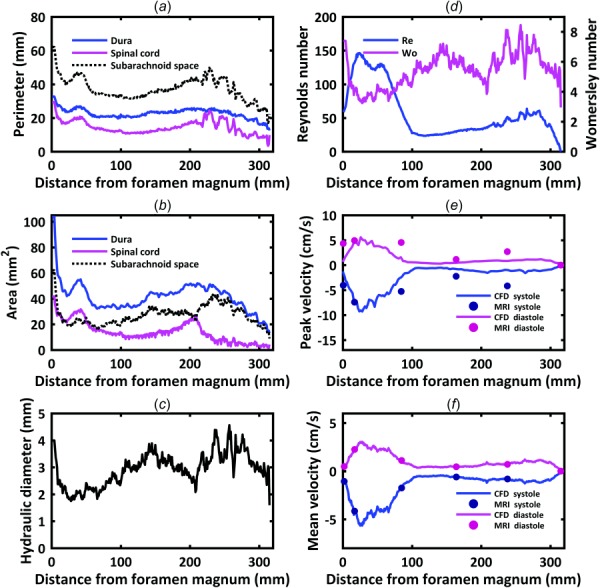
Hydrodynamic parameter distribution for the dura, spinal cord, and subarachnoid space computed along the spine for a cynomolgus monkey in terms of: (a) perimeter, (b) cross-sectional area, (c) hydraulic diameter, (d) Reynolds number, Re, and Womersley number, α. Comparison of CFD simulation (continuous line) and PCMRI measurements (dots) in terms of: (e) peak systolic and diastolic CSF velocity and (f) mean CSF velocity at peak systolic and diastolic flow.

Hydrodynamic Parameters.

Womersley number ranged from 8.45 to 2.95 (Table 4, Fig. 5(d)). Local maxima for Womersley number were present within the intrathecal sac (α = 8.4), thoracic enlargement (α = 7.1) and at the FM (α = 7.4). Womersley number had local minima within the cervical spine and just rostral to the intrathecal sac. Maximum Reynolds number was 149.9 and located in the cervical spine where CSF flow was maximum and the SAS had a relatively small hydraulic diameter.

CSF Flow.

Maximum peak and mean CSF velocities in the numerical model were present at 28 mm (∼C4–C5, Fig. 5(f)). Minimum value of peak and mean CSF velocities occurred in the lower lumbar spine and within the thoracic spine from 108 to 141 mm (∼T7–T10).

CSF flow oscillation had a decreasing magnitude and considerable variation in waveform shape along the spine (Fig. 6(a)). Spatial temporal distribution of CSF flow rate along the SAS showed that maximum CSF flow rate occurred caudal to C3–C4 at ∼30 mm (Fig. 6(b)). CSF flow rate waveform shape and magnitude was similar from ∼125 mm to the SAS termination. CSF PWV was quantified to be 1.19 m/s (Fig. 6(b)).

Fig. 6.

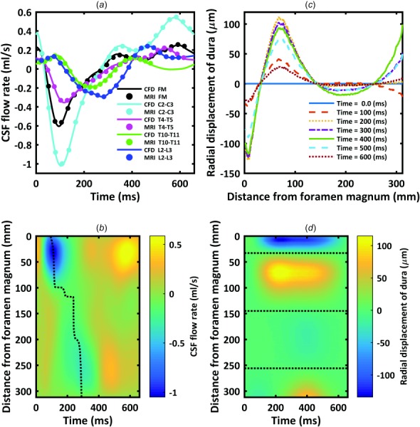
(a) CSF flow waveforms measured by PCMRI at five axial locations along the spine. Dots indicate experimental data and lines denote CFD results. Note: negative, or peak systolic, CSF flow is in the caudal direction. (b) Spatial-temporal distribution of the interpolated CSF flow rate along the spine. Dotted line indicates peak CSF flow rate at each axial level used to compute CSF PWV. (c) Radial displacement of the dura surface at 100 ms intervals over the CSF flow cycle. (d) Spatial-temporal distribution of the dura radial displacement along the spine. Dotted line indicates the three locations along the spine with zero radial motion of the dura.

Comparison of mean velocity at peak systolic flow at the five MRI slice locations (Fig. 5(f)) showed that MRI measurements were nearly identical to CFD results (error < 2.87%). Maximum percent difference in CFD versus MRI flow rate for all locations over the entire CSF flow cycle was 3.6% (Fig. 6(a)). Maximum percent difference in CFD versus MRI flow rate at peak systole was ∼2.8% (Table 5). Comparison of peak systolic and diastolic thru-plane CSF velocities at the five MRI slice locations (Fig. 5(e)) indicated that the MRI measurements had from 1.03 to 3.59× greater peak velocities compared to CFD.

Table 5.

Comparison of hydrodynamic CFD peak values with in vivo PCMRI measurements

Parameter	Location	CFD	MRI	% error
Qpeak-sys (ml/s)	FM	−0.61	−0.60	1.10
	C2-C3	−1.02	−1.00	2.20
	T4-T5	−0.35	−0.35	2.10
	T10-T11	−0.19	−0.19	2.87
L2-L3	−0.29	−0.29	0.60
Qpeak-dia (ml/s)	FM	0.25	0.26	1.87
	C2-C3	0.54	0.55	1.63
	T4-T5	0.22	0.22	1.39
	T10-T11	0.14	0.14	0.59
L2-L3	0.24	0.24	1.29

Note: V, velocity; Q, CSF flow rate; peak-sys, systolic peak flow; peak-dia, diastolic peak flow.

Dura Radial Displacement.

Radial displacement of the dura over the cardiac cycle is depicted in Fig. 6(c). Three axial locations at 55, 162, and 268 mm had zero radial displacement over the cardiac cycle. Also, different segments of the dura, with the exception of the lower lumbar spine, showed general trends in either positive or negative displacement. Spatial-temporal distribution of dura radial displacement (Fig. 6(d)) was different than CSF flow rate (Fig. 6(b)).

Comparison of CFD and In Vivo CSF Velocity Profiles.

Visual inspection of the PCMRI and CFD thru-plane velocity profiles at peak systole revealed large spatial differences (Fig. 7). Greater CSF velocities were observed by PCMRI in the anterior in comparison to the posterior space. In contrast, relatively uniform CSF flow profiles were simulated by CFD. All of the five sections showed CSF flow jets on PCMRI images. No such flow jets were present in the corresponding CFD velocity profiles. Epidural and vertebral artery blood flow was noted in the lumbar spine at L2–L3 and FM, respectively, as denoted by the black arrows at those locations (Fig. 7(d)). This flow was in close proximity to the CSF within the SAS and required omission in the MRI-based CSF flow waveform quantification.

Fig. 7.

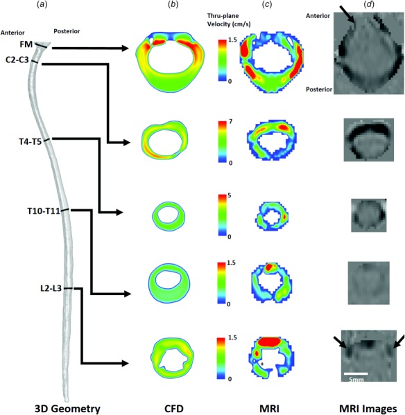
Peak-systolic thru-plane CSF velocity profiles simulated by CFD and measured by PCMRI for a cynomolgus monkey. (a) Overall view of the CFD model and slice locations. Note: different velocity scales are used at each slice location. (b) CSF velocity profiles at each slice location. (c) PCMRI visualization of CSF velocity profiles. + symbols indicate locations where spinal cord nerve roots appear to impact CSF flow profiles. (d) PCMRI gray scale images used to compute CSF flow waveforms. ↑ symbols highlight nearby regions with PCMRI signal that are not within the CSF space ROI (epidural venous flow at L2-L3, and vertebral artery flow at the FM).

Discussion

The delivery of therapeutic agents to the CNS tissue by the CSF is dependent on the following four stages: (1) pulsation-dependent mixing of the CSF, (2) arterial pulsation assisted transport along the perivascular spaces, (3) absorption from the perivascular space to the CNS tissue, and (4) extracellular transport and uptake into the neurons and along axons [6]. Each of these aspects must be understood to optimize CSF-based therapeutics. This study provides a flow model for accurate subject-specific reproduction of the nonuniform distribution of CSF flow along the entire spine using a nonuniform moving boundary approach. Results were verified by numerical independence studies and validated based on in vivo PCMRI measurements of CSF flow rates along the SAS.

Nonuniform CSF Flow Waveform Reproduction.

The distribution of CSF flow along the spine is nonuniform and shows local variations in waveform shape and magnitude (Fig. 1(b)). For example, CSF flow waveform amplitude was smaller at the FM compared to C2–C3 and then decreased at T4–T5 (Fig. 1(b)). Waveform amplitude was greater at L2–L3 compared to T10–T11. Thus, we implemented a nonuniform moving boundary approach to accurately reproduce the subject-specific MRI measurements. This involved an algorithm to compute local radial displacement of the dura (Fig. 3) and nearby mesh elements. The resulting CSF flow rate waveforms were compared to the in vivo measurements and shown to be nearly identical over the entire CSF flow cycle (Fig. 6(a)). In addition, comparison of mean velocity at peak systolic flow at the five MRI slice locations (Fig. 5(f)) showed that MRI measurements were nearly identical to CFD results (error < 2.87% at peak systolic CSF flow). To our knowledge, this model represents the first validation of numerically modeled subject-specific CSF flow rates along the entire spine. Increasing the mesh resolution would decrease the degree of error and also increase simulation time. Additional simulation time and computing resources should be considered carefully with respect to the clinical problem and specific questions.

A number of previous studies have simulated CSF flow along the spine under varying levels of complexity. Tangen et al. [18] used a dynamic mesh to simulate an axially phase-lagged version of the C4 CSF flow waveform measured by PCMRI. Agreement of CFD and MRI measurement of CSF flow rates at C4, T4, and L4 varied considerably depending on the axial location [18]. Another model by Sweetman et al. simulated CSF flow along the spine using a fluid–structure interaction approach with prescribed material properties of the dura. This model predicted a decreasing trend in CSF flux along the spine. Kuttler et al. [19] completed a semi-idealized model of CSF flow along the entire spine using a moving grid approach. Martin et al. completed a one-dimensional tube wave propagation model of CSF flow along the spine [1]. Bertram [20], Elliott [21], Cirovic and Kim [22], and Lockey et al. [23] also completed wave propagation models under varying degrees of geometric complexity. For all of these models, CSF flow or pressure was imposed at the model inlet but not validated based on in vivo CSF flow measurements.

Comparison of CFD and In Vivo CSF Velocity Profiles.

While the objective of our numerical modeling approach was to accurately reproduce the desired CSF flow rate distribution along the spine (Fig. 6(a)), the numerical model did not result in identical CSF velocity profiles as the in vivo PCMRI measurements. PCMRI showed axial CSF velocity profiles to be nonuniform with the presence of CSF flow jets and decreased CSF flow near nerve roots (Fig. 6(c)). Similar findings have been reported by others in the literature [24]. CFD velocity profiles at the same locations were relatively uniform. A number of numerical studies of CSF flow in the cervical spine in humans also found that CSF velocity profiles did not match in vivo PCMRI measurements [24,25]. In our study, agreement of peak CSF velocities was best at C2–C3 (error ∼7%, Fig. 5(e)). Maximum difference in peak CSF velocity at any location was 1.61 cm/s (Fig. 5(e)). This level of difference is likely within the range of noise present in the PCMRI signal that was collected with a velocity encoding of 10 cm/s.

The differences in velocity profiles and peak velocities between the PCMRI measurements and CFD simulations suggest that the level of anatomical detail in CFD simulations is not adequate to accurately model the CSF velocity profiles. A study by Pahlavian et al. showed that the discrepancy in CFD and PCMRI velocity profiles is not due to PCMRI measurement noise [26] or neural tissue motion over the cardiac cycle [27]. Taken together, these studies indicate that relatively small structures within the CSF flow field alter the CSF flow velocity profiles [28].

Unfortunately, the current 3T MR image resolution does not allow accurate reproduction of these relatively small anatomical structures such as spinal cord nerve roots, dorsal and dorsal lateral septum, arachnoid trabeculae, denticulate ligaments, and tiny blood vessels. These structures are likely the underlying reason for the differences in velocity profiles, in particular in the lower thoracic and lumbar spine (Fig. 7(c)). MR image resolution must improve to define these features in the future, for example, using 7T MRI [29]. Our geometric model did not include these small structures as they are not possible to image on a subject-specific basis. However, they should be included to accurately reproduce in vivo CSF flow profiles.

It is likely that accurate subject-specific reproduction of CSF flow rate distribution and velocity profiles is needed to model subject-specific intrathecal solute transport. Alternatively, one may choose to create idealized models with these structures included that can help inform intrathecal device design and protocol development. In any case, these models should have accurate distribution of nonuniform CSF flow along the spine. Our approach satisfies that need.

CSF Space Geometry Quantification.

To our knowledge, axial variation in spinal SAS geometry in terms of A_cs, P_cs, and D_H in a cynomolgus monkey has not been reported in the literature. This is likely due to the relatively long time period (55 min total) required to obtain the high-resolution MRI images (375 μm isotopic) used to segment the CSF space in this study. Hydraulic diameter ranged from ∼1.5 to 4.5 mm in the NHP analyzed. The axial distribution of SAS geometry in the cynomolgus monkey had a similar trend as that quantified in humans for A_cs, P_cs, and D_H [9], albeit approximately ∼7.4, 2.3, and 2.4× smaller, respectively, in magnitude compared to a human [15]. Total CSF volume in the spine for the cynomolgus monkey in this study was ∼8.7 ml. Based on Loth et al. human spinal CSF volume can be estimated to be ∼125 ml. Detailed MR investigation of the complete spinal CSF space in terms of its geometry is lacking in the literature.

Importance of Hydrodynamic Parameters.

The analysis of Reynolds and Womersley numbers is helpful to compare the present study results with the literature and validate the CFD methodology assumptions, such as laminar flow. Using the peak CSF flow rate and hydraulic diameter, Re did not exceed 150 for any axial location along the NHP spine (Fig. 5(d)). Re for the NHP analyzed in our study was consistent with previous findings for humans that quantified Re to range from ∼150 to 450 [15]. In this study, Re was significantly lower than the critical value for transition to turbulence for flow in a straight circular pipe and thus, we expect the flow to be laminar throughout the SAS. However, a study by Helgeland et al. indicated that CSF flow may have instabilities [30]. The phase-contrast MRI measurements used to detect the CSF velocity profiles in our study were time-averaged over multiple cardiac cycles. Thus, any unsteadiness in pixel velocities that could be due to flow instability was not possible to detect.

Our findings indicated that maximum Re was present at C4–C5. This location may be best suited for intrathecal delivery of solutes [6]. However, intrathecal drug delivery at C4–C5 may have increased risk for CNS tissue damage in comparison to the typical delivery location in the lumbar spine. It is unclear if this location would be the same for humans, as little information is known about CSF flow rates along the entire spine in humans.

Womersley number, α, ranged from ∼3 to 8, suggesting that transient inertial forces were dominant over viscous forces. These findings are in agreement with the range of Womersley numbers for CSF flow in humans [11]. They also indicate that viscous effects within the spinal SAS are relatively insignificant as documented by Loth et al. [15].

CSF Pulse Wave Velocity Along the Spine (PWV).

Spatial-temporal smoothing of the in vivo measured CSF flow rate waveforms showed that the CSF flow has a distinguishable wave propagation velocity (PWV) along the SAS of approximately 1.19 m/s (Fig. 6(b)). This PWV is lower than previously reported in the literature for humans, albeit, the number of in vivo studies is limited. An in vivo study by Kalata et al. used high-speed PCMRI to quantify the CSF velocity wave speed in a ∼20 cm portion of the cervical spine and found it to be 4.6 ± 1.7 m/s at systole in healthy subjects [17]. A fluid–structure interaction study by Sweetman and Linninger predicted spinal CSF PWV to be ∼3 m/s [31]. Another simulation by Martin et al. used a numerical 1D tube model of the spinal SAS to parametrically alter the dura mechanical properties and analyze the effect on spinal CSF flow and pressures [32]. In that study, CSF PWV varied from 2.5 to 13.5 m/s depending on dura elasticity. Martin et al. also investigated CSF wave phenomena in the spine using in vitro models and found CSF wave reflections to be present [1]. Similar findings have been found numerically by a number of investigators using a number of approaches [20,33]. Our results did not show a large degree of CSF wave reflection within the spine (Fig. 6(b)). More detailed investigation is needed to understand CSF PWV in the spine and its relevance, if any, to CNS disease pathophysiology and intrathecal therapeutics.

Motion of the Dura.

To our knowledge, radial motion of the dura has not been directly measured along the spine using MR imaging, likely due to the relatively small degree of motion present in that tissue. Our results indicate that a maximum radial dura displacement of ∼135 μm (Fig. 6(c)) is sufficient to reproduce the measured CSF flow rates along the NHP spine (Fig. 6(a)). Interestingly, there were three axial locations along the spine that did not have dura radial displacement (Fig. 6(d), dotted lines). The location of maximum dura displacement was at the T3–T4 and C1–C2 vertebral level (Table 3). These locations had a positive and negative displacement from baseline, respectively. Maximum CSF flow rate was present between these two locations at approximately C3–C4. CSF flow wave propagation and dura displacement did not appear to be coupled in terms of their spatial temporal distribution (compare Figs. 6(c) and 6(d)).

Limitations

The numerical modeling methods in this study were based on MRI measurements for a single cynomolgus monkey. Geometric and hydrodynamic findings were presented to understand the hydrodynamic environment. These parameters should be investigated in a larger group of NHPs to determine their statistical variance with gender, among NHP species and comparison to humans.

A single operator accomplished geometric segmentation of the MRI images used in this study. A study by Martin et al. indicated a high degree of reliability in CFD results for geometries produced by different operators [11]. We therefore expect the trends in CSF dynamics and geometry to be similar, given a different operator. Nonuniform motion of the numerical mesh was defined by the measured CSF flow rate using a manual region of interests (ROI) selection. Careful attention was given to omit regions outside of the SAS by referencing the high-resolution T2-weighted image sets (e.g., for omission of epidural venous flow around the dura). Pixels with net flow in one direction were omitted (blood flow), and pixels with oscillatory flow were included (CSF). Nevertheless, in some cases, it was difficult to distinguish CSF flow from nearby epidural flow that may pulsate.

Our modeling approach did not include CSF within the SAS of the brain or ventricles because we did not have MR images of flow or geometry obtained within those regions for validation of the numerical model. These images were not possible to collect in the already relatively long 1 h and 21 min MRI measurement timeframe. Additionally, the presented model used a moving boundary method in which boundary motion was prescribed at the model wall. This model did not account for fluid structure interaction (FSI) of the wall (tissues) and fluid. Prescribed motion of the dura allowed reproduction of the in vivo measured CSF flow rate.

Conclusion

This study presents a flow model based on a nonuniform moving boundary method to accurately reproduce in vivo CSF flow rate distribution and waveform along the spinal SAS of a cynomolgus monkey. Maximum error measured at peak CSF flow rate in the numerical model was <3.6%. Deformation of the dura ranged up to a maximum of 135 μm. MRI measurements of CSF space geometry and flow were successfully acquired to define the numerical domain and boundary conditions. For the single cynomolgus monkey analyzed, results showed that CSF flow was laminar with a peak Reynolds number of ∼150 and average Womersley number of ∼5.4. Geometric analysis indicated that total spinal CSF space volume was ∼8.7 ml. Average hydraulic diameter, wetted perimeter, and SAS area were 2.9 mm, 37.3 mm, and 27.2 mm², respectively. CSF PWV along the spine was quantified to be 1.2 m/s and did not appear to have a significant degree of wave reflection at the spine termination. Maximum CSF flow movement was present at the C4–C5 vertebral level. In combination, these results represent the first CFD simulation of spinal CSF hydrodynamics in a monkey.

Nomenclature

A =

area

CFD =

computational fluid dynamics

CNS =

central nervous system

CSF =

cerebrospinal fluid

CT =

cycle time

D_H =

hydraulic diameter

df =

flow rate variation

dh =

segment height

dr =

radial deformation

ECG =

electrocardiogram

FM =

foramen magnum

FSI =

fluid-structure interaction

h =

height

HR =

heart rate

IACUC =

Institutional Animal Care and Use Committee

MRI =

magnetic resonance imaging

NHP =

nonhuman primate

P =

perimeter

PCMRI =

phase-contrast magnetic resonance imaging

Q =

flow rate

r =

radius

Re =

Reynolds number

ROI =

region of interests

SAS =

subarachnoid space

SC =

spinal cord

t =

time

T =

tesla

V =

velocity

3D =

three-dimensional

α =

Womersley number, dimensionless

θ =

angle, deg

μ =

dynamic viscosity, Pa·s

ν =

kinematic viscosity, m²s⁻¹

ρ =

density, kg/m³

ω =

angular frequency, rad/s

References

- [1]. Martin, B. A. , Labuda, R. , Royston, T. J. , Oshinski, J. N. , Iskandar, B. , and Loth, F. , 2010, “ Spinal Subarachnoid Space Pressure Measurements in an In Vitro Spinal Stenosis Model: Implications on Syringomyelia Theories,” ASME J. Biomech. Eng., 132(11), p. 111007. 10.1115/1.4000089 [DOI] [PubMed] [Google Scholar]
- [2]. Wostyn, P. , Audenaert, K. , and De Deyn, P. P. , 2009, “ More Advanced Alzheimer's Disease May Be Associated With a Decrease in Cerebrospinal Fluid Pressure,” Cerebrospinal Fluid Res., 6(1), p. 1. 10.1186/1743-8454-6-14 [DOI] [PMC free article] [PubMed] [Google Scholar]
- [3]. Bunck, A. C. , Kroeger, J. R. , Juettner, A. , Brentrup, A. , Fiedler, B. , Crelier, G. R. , Martin, B. A. , Heindel, W. , Maintz, D. , and Schwindt, W. , 2012, “ Magnetic Resonance 4D Flow Analysis of Cerebrospinal Fluid Dynamics in Chiari I Malformation With and Without Syringomyelia,” Eur. Radiol., 22(9), pp. 1860–1870. 10.1007/s00330-012-2457-7 [DOI] [PubMed] [Google Scholar]
- [4]. Bradley, W. G., Jr. , Scalzo, D. , Queralt, J. , Nitz, W. N. , Atkinson, D. J. , and Wong, P. , 1996, “ Normal-Pressure Hydrocephalus: Evaluation With Cerebrospinal Fluid Flow Measurements at MR Imaging,” Radiology, 198(2), pp. 523–529. 10.1148/radiology.198.2.8596861 [DOI] [PubMed] [Google Scholar]
- [5]. Simpson, K. , Baranidharan, G. , and Gupta, S. , 2012, Spinal Interventions in Pain Management, Oxford University Press, Oxford, UK. [Google Scholar]
- [6]. Papisov, M. I. , Belov, V. V. , and Gannon, K. S. , 2013, “ Physiology of the Intrathecal Bolus: The Leptomeningeal Route for Macromolecule and Particle Delivery to CNS,” Mol. Pharmaceutics, 10(5), pp. 1522–1532. 10.1021/mp300474m [DOI] [PMC free article] [PubMed] [Google Scholar]
- [7]. Xie, L. , Kang, H. , Xu, Q. , Chen, M. J. , Liao, Y. , Thiyagarajan, M. , O'Donnell, J. , Christensen, D. J. , Nicholson, C. , Iliff, J. J. , Takano, T. , Deane, R. , and Nedergaard, M. , 2013, “ Sleep Drives Metabolite Clearance From the Adult Brain,” Science, 342(6156), pp. 373–377. 10.1126/science.1241224 [DOI] [PMC free article] [PubMed] [Google Scholar]
- [8]. Weller, R. O. , Djuanda, E. , Yow, H. Y. , and Carare, R. O. , 2009, “ Lymphatic Drainage of the Brain and the Pathophysiology of Neurological Disease,” Acta Neuropathol., 117(1), pp. 1–14. 10.1007/s00401-008-0457-0 [DOI] [PubMed] [Google Scholar]
- [9]. Martin, B. A. , Kalata, W. , Shaffer, N. , Fischer, P. , Luciano, M. , and Loth, F. , 2013, “ Hydrodynamic and Longitudinal Impedance Analysis of Cerebrospinal Fluid Dynamics at the Craniovertebral Junction in Type I Chiari Malformation,” PloS One, 8(10), p. e75335. 10.1371/journal.pone.0075335 [DOI] [PMC free article] [PubMed] [Google Scholar]
- [10]. Martin, B. A. , Kalata, W. , Loth, F. , Royston, T. J. , and Oshinski, J. N. , 2005, “ Syringomyelia Hydrodynamics: An In Vitro Study Based on In Vivo Measurements,” ASME J. Biomech. Eng., 127(7), pp. 1110–1120. 10.1115/1.2073687 [DOI] [PubMed] [Google Scholar]
- [11]. Martin, B. A. , Yiallourou, T. I. , Pahlavian, S. H. , Thyagaraj, S. , Bunck, A. C. , Loth, F. , Sheffer, D. B. , Kroger, J. R. , and Stergiopulos, N. , 2016, “ Inter-Operator Reliability of Magnetic Resonance Image-Based Computational Fluid Dynamics Prediction of Cerebrospinal Fluid Motion in the Cervical Spine,” Ann. Biomed. Eng., 44(5), pp. 1524–1537. 10.1007/s10439-015-1449-6 [DOI] [PMC free article] [PubMed] [Google Scholar]
- [12]. Yiallourou, T. , Schmid Daners, M. , Kurtcuoglu, V. , Haba-Rubio, J. , Heinzer, R. , Fornari, E. , Santini, F. , Sheffer, D. B. , Stergiopulos, N. , and Martin, B. A. , 2015, “ Continuous Positive Airway Pressure Alters Cranial Blood Flow and Cerebrospinal Fluid Dynamics at the Craniovertebral Junction,” Interdiscip. Neurosurg., 2(3), pp. 152–159. 10.1016/j.inat.2015.06.004 [DOI] [Google Scholar]
- [13]. Gupta, A. , Church, D. , Barnes, D. , and Hassan, A. , 2009, “ Cut to the Chase: On the Need for Genotype-Specific Soft Tissue Sarcoma Trials,” Ann. Oncol., 20(3), pp. 399–400. 10.1093/annonc/mdp021 [DOI] [PubMed] [Google Scholar]
- [14]. Gupta, S. , Soellinger, M. , Grzybowski, D. M. , Boesiger, P. , Biddiscombe, J. , Poulikakos, D. , and Kurtcuoglu, V. , 2010, “ Cerebrospinal Fluid Dynamics in the Human Cranial Subarachnoid Space: An Overlooked Mediator of Cerebral Disease—I: Computational Model,” J. R. Soc. Interface, 7(49), pp. 1195–1204. 10.1098/rsif.2010.0033 [DOI] [PMC free article] [PubMed] [Google Scholar]
- [15]. Loth, F. , Yardimci, M. A. , and Alperin, N. , 2001, “ Hydrodynamic Modeling of Cerebrospinal Fluid Motion Within the Spinal Cavity,” ASME J. Biomech. Eng., 123(1), pp. 71–79. 10.1115/1.1336144 [DOI] [PubMed] [Google Scholar]
- [16]. San, O. , and Staples, A. E. , 2012, “ An Improved Model for Reduced-Order Physiological Fluid Flows,” J. Mech. Med. Biol., 12(3), p. 1250052. 10.1142/S0219519411004666 [DOI] [Google Scholar]
- [17]. Kalata, W. , Martin, B. A. , Oshinski, J. N. , Jerosch-Herold, M. , Royston, T. J. , and Loth, F. , 2009, “ MR Measurement of Cerebrospinal Fluid Velocity Wave Speed in the Spinal Canal,” IEEE Trans. Biomed. Eng., 56(6), pp. 1765–1768. 10.1109/TBME.2008.2011647 [DOI] [PubMed] [Google Scholar]
- [18]. Tangen, K. M. , Hsu, Y. , Zhu, D. C. , and Linninger, A. A. , 2015, “ CNS Wide Simulation of Flow Resistance and Drug Transport Due to Spinal Microanatomy,” J. Biomech., 48(10), pp. 2144–2154. 10.1016/j.jbiomech.2015.02.018 [DOI] [PubMed] [Google Scholar]
- [19]. Kuttler, A. , Dimke, T. , Kern, S. , Helmlinger, G. , Stanski, D. , and Finelli, L. A. , 2010, “ Understanding Pharmacokinetics Using Realistic Computational Models of Fluid Dynamics: Biosimulation of Drug Distribution Within the CSF Space for Intrathecal Drugs,” J. Pharmacokinet. Pharmacodyn., 37(6), pp. 629–644. 10.1007/s10928-010-9184-y [DOI] [PMC free article] [PubMed] [Google Scholar]
- [20]. Bertram, C. D. , 2010, “ Evaluation by Fluid/Structure-Interaction Spinal-Cord Simulation of the Effects of Subarachnoid-Space Stenosis on an Adjacent Syrinx,” ASME J. Biomech. Eng., 132(6), p. 061009. 10.1115/1.4001165 [DOI] [PubMed] [Google Scholar]
- [21]. Elliott, N. S. , 2012, “ Syrinx Fluid Transport: Modeling Pressure-Wave-Induced Flux Across the Spinal Pial Membrane,” ASME J. Biomech. Eng., 134(3), p. 031006. 10.1115/1.4005849 [DOI] [PubMed] [Google Scholar]
- [22]. Cirovic, S. , and Kim, M. , 2012, “ A One-Dimensional Model of the Spinal Cerebrospinal-Fluid Compartment,” ASME J. Biomech. Eng., 134(2), p. 021005. 10.1115/1.4005853 [DOI] [PubMed] [Google Scholar]
- [23]. Lockey, P. , Poots, G. , and Williams, B. , 1975, “ Theoretical Aspects of the Attenuation of Pressure Pulses Within Cerebrospinal-Fluid Pathways,” Med. Biol. Eng., 13(6), pp. 861–869. 10.1007/BF02478090 [DOI] [PubMed] [Google Scholar]
- [24]. Yiallourou, T. I. , Kroger, J. R. , Stergiopulos, N. , Maintz, D. , Martin, B. A. , and Bunck, A. C. , 2012, “ Comparison of 4D Phase-Contrast MRI Flow Measurements to Computational Fluid Dynamics Simulations of Cerebrospinal Fluid Motion in the Cervical Spine,” PLoS One, 7(12), p. e52284. 10.1371/journal.pone.0052284 [DOI] [PMC free article] [PubMed] [Google Scholar]
- [25]. Heidari Pahlavian, S. , Bunck, A. C. , Loth, F. , Shane Tubbs, R. , Yiallourou, T. , Kroeger, J. R. , Heindel, W. , and Martin, B. A. , 2015, “ Characterization of the Discrepancies Between Four-Dimensional Phase-Contrast Magnetic Resonance Imaging and In-Silico Simulations of Cerebrospinal Fluid Dynamics,” ASME J. Biomech. Eng., 137(5), p. 051002. 10.1115/1.4029699 [DOI] [PMC free article] [PubMed] [Google Scholar]
- [26]. Pahlavian, S. H. , Bunck, A. C. , Thyagaraj, S. , Giese, D. , Loth, F. , Hedderich, D. M. , Kroeger, J. R. , and Martin, B. A. , 2016, “ Accuracy of 4D Flow Measurement of Cerebrospinal Fluid Dynamics in the Cervical Spine: An In Vitro Verification Against Numerical Simulation,” Ann. Biomed. Eng., 44(11), pp. 3202–3214. 10.1007/s10439-016-1602-x [DOI] [PMC free article] [PubMed] [Google Scholar]
- [27]. Pahlavian, S. H. , Loth, F. , Luciano, M. , Oshinski, J. , and Martin, B. A. , 2015, “ Neural Tissue Motion Impacts Cerebrospinal Fluid Dynamics at the Cervical Medullary Junction: A Patient-Specific Moving-Boundary Computational Model,” Ann. Biomed. Eng., 43(12), pp. 2911–2923. 10.1007/s10439-015-1355-y [DOI] [PMC free article] [PubMed] [Google Scholar]
- [28]. Heidari Pahlavian, S. , Yiallourou, T. , Tubbs, R. S. , Bunck, A. C. , Loth, F. , Goodin, M. , Raisee, M. , and Martin, B. A. , 2014, “ The Impact of Spinal Cord Nerve Roots and Denticulate Ligaments on Cerebrospinal Fluid Dynamics in the Cervical Spine,” PLoS One, 9(4), p. e91888. 10.1371/journal.pone.0091888 [DOI] [PMC free article] [PubMed] [Google Scholar]
- [29]. Sigmund, E. E. , Suero, G. A. , Hu, C. , McGorty, K. , Sodickson, D. K. , Wiggins, G. C. , and Helpern, J. A. , 2012, “ High-Resolution Human Cervical Spinal Cord Imaging at 7 T,” NMR Biomed., 25(7), pp. 891–899. 10.1002/nbm.1809 [DOI] [PMC free article] [PubMed] [Google Scholar]
- [30]. Helgeland, A. , Mardal, K. A. , Haughton, V. , and Reif, B. A. , 2014, “ Numerical Simulations of the Pulsating Flow of Cerebrospinal Fluid Flow in the Cervical Spinal Canal of a Chiari Patient,” J. Biomech., 47(5), pp. 1082–1090. 10.1016/j.jbiomech.2013.12.023 [DOI] [PubMed] [Google Scholar]
- [31]. Sweetman, B. , and Linninger, A. A. , 2011, “ Cerebrospinal Fluid Flow Dynamics in the Central Nervous System,” Ann. Biomed. Eng., 39(1), pp. 484–496. 10.1007/s10439-010-0141-0 [DOI] [PubMed] [Google Scholar]
- [32]. Martin, B. A. , Reymond, P. , Novy, J. , Baledent, O. , and Stergiopulos, N. , 2012, “ A Coupled Hydrodynamic Model of the Cardiovascular and Cerebrospinal Fluid System,” Am. J. Physiol. Heart Circ. Physiol., 302(7), pp. H1492–H1509. 10.1152/ajpheart.00658.2011 [DOI] [PubMed] [Google Scholar]
- [33]. Elliott, N. S. J. , Bertram, C. D. , Martin, B. A. , and Brodbelt, A. R. , 2013, “ Syringomyelia: A Review of the Biomechanics,” J. Fluids Struct., 40, pp. 1–24. 10.1016/j.jfluidstructs.2013.01.010 [DOI] [Google Scholar]