A MAD-Bayes Algorithm for State-Space Inference and Clustering with Application to Querying Large Collections of ChIP-Seq Data Sets

Abstract

Current analytic approaches for querying large collections of chromatin immunoprecipitation followed by sequencing (ChIP-seq) data from multiple cell types rely on individual analysis of each data set (i.e., peak calling) independently. This approach discards the fact that functional elements are frequently shared among related cell types and leads to overestimation of the extent of divergence between different ChIP-seq samples. Methods geared toward multisample investigations have limited applicability in settings that aim to integrate 100s to 1000s of ChIP-seq data sets for query loci (e.g., thousands of genomic loci with a specific binding site). Recently, Zuo et al. developed a hierarchical framework for state-space matrix inference and clustering, named MBASIC, to enable joint analysis of user-specified loci across multiple ChIP-seq data sets. Although this versatile framework estimates both the underlying state-space (e.g., bound vs. unbound) and also groups loci with similar patterns together, its Expectation-Maximization-based estimation structure hinders its applicability with large number of loci and samples. We address this limitation by developing MAP-based asymptotic derivations from Bayes (MAD-Bayes) framework for MBASIC. This results in a K-means-like optimization algorithm that converges rapidly and hence enables exploring multiple initialization schemes and flexibility in tuning. Comparison with MBASIC indicates that this speed comes at a relatively insignificant loss in estimation accuracy. Although MAD-Bayes MBASIC is specifically designed for the analysis of user-specified loci, it is able to capture overall patterns of histone marks from multiple ChIP-seq data sets similar to those identified by genome-wide segmentation methods such as ChromHMM and Spectacle.

1. Introduction

Many large consortia (e.g., ENCODE [The ENCODE Project Consortium, 2012], REMC [Roadmap Epigenomics Consortium, 2015]) as well as investigator-initiated projects generated large collections of chromatin immunoprecipitation followed by sequencing (ChIP-seq) data profiling multiple proteins and histone modifications across a wide variety of systems. Most current approaches for analyzing data from multiple cell types perform initial analyses such as peak calling in ChIP-seq independently in each cell/tissue/treatment type. This approach ignores the fact that functional elements are frequently shared between related cell types and leads to an overestimation of the extent of functional divergence between the conditions. Although the uniform processing pipelines developed by data-generating consortia and the resulting analysis of consortia data enable easy access to these data, joint analysis approaches that take advantage of the inherent relationships between data sets and cell types are required. Joint inference for ChIP-seq data sets can be formulated as inferring for each locus whether or not it exhibits ChIP-seq signal in a given condition and also grouping loci based on their profile similarity across multiple samples.

It is now widely accepted that joint analysis of these types of data can uncover signals that are otherwise too small to detect from a single experiment (Bardet et al., 2012; Bao et al., 2013). Among the available joint analysis methods, jMOSAiCS (Zeng et al., 2013) builds on ChIP-seq peak-caller MOSAiCS (Kuan et al., 2011) and incorporates a multilayer hidden states model that governs the relationship of enrichment among different samples. Bao et al. (2014 utilize a one-dimensional Markov random field model to account for spatial dependencies along the genome while modeling individual components by mixtures of Zero Inflated Poisson or Negative Binomial models. dCaP (Chen et al., 2014) uses a three-step log-likelihood ratio test to jointly identify binding events in multiple experimental conditions. ChromHMM (Ernst and Kellis, 2010) and Segway (Hoffman et al., 2012) are two commonly adopted approaches for segmenting the genome into chromatin states based on histone ChIP-seq and rely on hidden Markov models (HMMs) and Bayesian Networks, respectively. Recently, Spectacle (Song and Chen, 2015) provided a transformative improvement of ChromHMM by utilizing spectral learning for parameter estimation in HMMs. hiHMM (Sohn et al., 2015) uses a Bayesian nonparametric formulation of the HMMs while taking into account species-specific biases.

Overall, available strategies for considering multiple ChIP-seq data sets simultaneously can be broadly classified based on (i) whether or not they can deal with only transcription factors (TFs) (Liang and Keleş, 2012; Mahony et al., 2014), only histone modifications (Ernst and Kellis, 2010; Song and Smith, 2011; Ferguson et al., 2012; Hoffman et al., 2012; Song and Chen, 2015), or both (Bao et al., 2013; Zeng et al., 2013) types of ChIP-seq data; (ii) whether or not they rely on a priori analysis of individual data sets (Ernst and Kellis, 2010; Ferguson et al., 2012; Liang and Keleş, 2012; Mahony et al., 2014; Song and Chen, 2015), (iii) whether or not they focus on differential occupancy and can handle very few number of conditions (Taslim et al., 2011; Liang and Keleş, 2012; Ji et al., 2013), (iv) whether or not they can scale up to 100s to 1000s of data sets. These approaches, with the potential exception of Song and Chen (2015), do not scale up to 100s to 1000s of data sets because they, to a large extent, utilize variants of hidden Markov models and/or implement variants of the Expectation-Maximization (EM) algorithm (Dempster et al., 1977) for parameter estimation. Furthermore, none of these approaches accommodate querying of multiple data sets for selected loci. Their analysis results serve to “annotate” user-specified loci without any notion of uncertainty.

We recently introduced MBASIC (Zuo et al., 2016) as a probabilistic method for querying multiple ChIP-seq data sets jointly for user-specified loci. When multiple ChIP-seq data sets (multiple TFs profiled in different cell/tissue types under a variety of conditions) are available, the key inference encompasses both identifying peaks in individual data sets (state-space mapping) and identifying groups of loci that cluster across different experiments (state-space clustering). At the core of MBASIC are biologically validated and commonly adapted models for measurements from individual experiments (e.g., read data models from Kuan et al., 2011, and Zuo and Keleş, 2014 for state-space mapping) and a mixture model for clustering of the loci with similar state-space mapping. Parameter estimation in this versatile model is based on the EM algorithm and hence does not scale up with large number of user-specified loci and ChIP-seq data sets.

In this article, we adopt a small-variance asymptotics framework for MBASIC and derive a K-means-like MAP-based asymptotic derivations from Bayes (MAD-Bayes) algorithm (Broderick et al., 2013). This alternative estimation framework for MBASIC targets at large-scale data sets and genomic loci. Specifically, we consider a mixture of Log-normal distributions for state-specific observations with a Chinese Restaurant Process (CRP) (Blackwell and MacQueen, 1973; Aldous, 1983) as the clustering prior. Small-variance asymptotics for maximizing the posterior distribution leads to a K-means like objective function with a key penalty term for the number of clusters. Extensive comparisons with MBASIC indicate that this approach can significantly speed up model estimation without significant impact on the estimation performance. Although methods such as ChromHMM and Spectacle inherently have a different purpose than MAD-Bayes MBASIC, we compared the three on histone ChIP-seq data from GM12878 cells. This comparison indicated that MAD-Bayes MBASIC can capture the overall patterns that these segmentation methods identify.

2. Methods

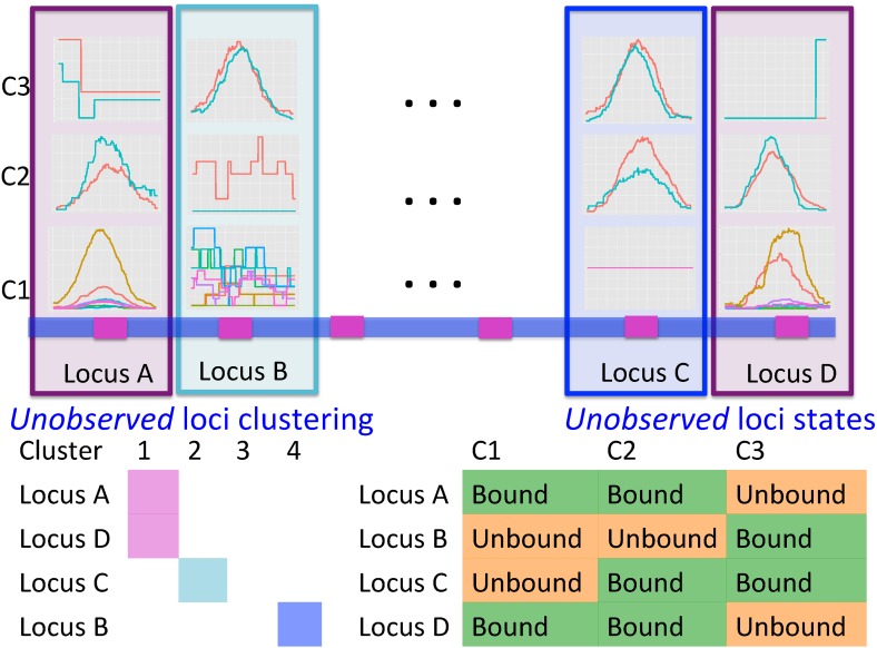
We begin our exposition with an overall description of the Bayesian MBASIC model (Fig. 1) and then derive the MAD-Bayes algorithm. Some key aspects of our approach are model initialization and tuning parameter selection. Although these aspects arise in all of the already mentioned joint analysis methods, they are typically not well studied because of computational costs.

FIG. 1.

Overview of the MBASIC modeling framework. Curves within each panel depict different replicates under the experimental conditions C1, C2, and C3. Loci A and D are in the same cluster.

2.1. The Bayesian MBASIC model

We consider I genomic loci of interest, indexed from , from the reference genome with observations from K different experimental conditions. We use the notion of loci loosely in the sense that these loci could correspond to promoter regions of genes (all or members of specific pathways), locations of genome with a specific TF binding motif, or peaks from a specific ChIP-seq experiment. The K conditions denote different TFs and cell/tissue types. Then, the key inference concerns analyzing I loci based on these K experiments.

To further motivate the circumstances this inference problem arises, we consider an example from GATA-factor biology. In Hewitt et al. (2015), we were interested in an overall analysis of all the E-box-GATA composite elements based on all the ENCODE ChIP-seq data to identify sites similar to the functional E-box-GATA composite element at the +9.5 loci that is causal for MonoMAC disease (a rare genetic disorder associated with myelodysplasia, cytogenetic abnormalities, and myeloid leukemias) (Johnson et al., 2012). The E-box-GATA composite elements are represented by CANNTGN{6-14}AGATAA oligonucleotides, where N denotes any nucleotide and N{6-14} denotes any nucleotide sequence of length 6 to 14 bps, and are found abundantly in the genome, for example, hg19 harbors K of them. Joint analysis of these loci over, for example, all the available ENCODE TF ChIP-seq data sets ( based on www.encodeproject.org) to identify groups of loci that are similar to the +9.5 element represents one potential application. In the MBASIC framework, the binding states are governed by a clustering structure, which groups genomic loci with similar overall binding states across experiments together. For the E-box-GATA composite elements example, in addition to the binding states for each candidate loci across experiments, MBASIC also reports a clustering of loci based on the binding states. The cluster with the +9.5 loci harbors candidate E-box-GATA elements to follow up Hewitt et al. (2015).

Let n_k denote the number of experimental replicates for the k-th condition. We denote the observation for the i-th locus under condition k for the l-th replicate by , for , , and . We assume that a latent state is associated with the i-th locus and the k-th condition. is the indicator for the state to be s, where s takes values in a discrete state-space . In a ChIP-seq experiment, we typically have , where or indicates that the i-th locus is unenriched (unbound) or enriched (bound) under condition k, respectively. Our model consists of two key components. The first component, state-space mapping, assumes the following distribution of conditional on :

where f_s is a density function. Its parameters , , and denote covariates encoding known information for locus i. Note that carries information related to how the counts for unenriched loci arise (when ), that is, data from control input experiments, guanine-cytosine (GC) content, and mappability (Zuo and Keleş, 2014). In this article, we take f_s to be Log-normal distribution to represent ChIP-seq read counts after potential normalization for mappability and GC content:

where we utilize conjugate priors and .

The second part of the Bayesian MBASIC model is state-space clustering. We assume that the loci can be clustered into J groups denoted by , that is, . Let if the i-th locus belongs to cluster j and 0 otherwise. The states for the loci within the same cluster follow a product multinomial distribution:

with noninformative prior . We further assume a CRP (Aldous, 1983) as a prior for the number of clusters J. Let be a hyperparameter of the model. The first locus forms C₁ at the start and each locus gets assigned to a cluster recursively. Suppose we have assigned loci to clusters. The i-th locus is then assigned to with probability proportional to the size of . It can also form a new cluster with probability proportional to . Then, the prior density for a partition with J clusters is

With these specifications, we can derive the posterior density of the model for parameter estimation. Although the resulting posterior density leads to a Gibbs sampling algorithm, such a Gibbs sampling scheme requires excessive computational time for mixing (data not shown). Therefore, we derive a MAD-Bayes algorithm by utilizing small-variance asymptotics.

2.2. MAD-Bayes algorithm

We further make the following small-variance assumptions for the MBASIC model:

Assumption 1. All data sets have equal variance: .

Assumption 2. For a given cluster and condition, one of the hidden states dominates with for .

Assumption 3. for .

Proposition 1. Under 1, 2, 3, and as , the posterior density reduces to

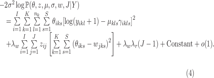This proposition implies that the MAP estimate of the MBASIC framework with CRP and Log-normal mixture model is asymptotically equivalent to the solution of the following optimization problem:

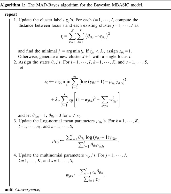
where the objective function can be viewed as a weighted loss function that integrates the state inference error from Log-normal density as the first term, the clustering error as the second term, and the cost for creating new clusters as the third term. Here, and are tuning parameters that ensure that the cluster assignments are nontrivial. The equal-variance assumption is inherently quite strong for ChIP-seq data; however, it was recently shown to work well as a first approximation in a differential ChIP-seq analysis context (Ji et al., 2013). We next derive the MAD-Bayes algorithm to generate a local solution for this minimization problem (Algorithm 1).

We note that each step of this algorithm does not increase the objective function in Equation (5), and the updates for 's and 's minimize the objective function for a fixed configuration of 's and 's. Moreover, there are finite number of combinations for 's and 's such that no cluster is empty and all clusters are distinct from one another. With such observations, we conclude the convergence of this algorithm.

Proposition 2. Algorithm 1 converges after a finite number of iterations to a local minimum of the objective function in Equation (5).

2.3. Model initialization

Similar to the EM algorithm variants for HMMs, the MAD-Bayes algorithm for MBASIC also converges to a local solution and hence can be sensitive to initial starting values. We present a guided two-stage initialization strategy for the states and clusters to attenuate the impact of initialization. We start from initialization of the states by minimizing the state inference error [the first term in Eq. (5)], which has a degenerate form if :

Therefore, we use Algorithm 1 by setting to initialize 's and 's.

We utilize these initial values of 's and consider three options for the cluster initialization (i.e., 's and 's): K-means, K-means++, and Adaptive K-means++, where the first two require a predetermined number of clusters J, which we discuss in Section 2.4. The K-means option runs hard K-means algorithm on the 's, whereas the K-means++ option assigns a cluster label to each unit i with probability inversely proportional to its distance to the current clusters . The adaptive K-means initialization uses a K-means++ style, but increases the number of clusters from , until the value of the function in Equation (7) does not decrease.

2.4. Selecting the tuning parameters

We note that the CRP prior for the number of clusters and the small-variance asymptotics assumptions introduce tuning parameters for the MAD-Bayes algorithm (Algorithm 1). Even for the models with one tuning parameter, Broderick et al. (2013) acknowledged the difficulty in choosing their appropriate values in practice. Hence, we propose an empirically motivated method for tuning parameter selection. In practice, we do not expect our small-variance assumption as to hold rigidly for real data; however, we expect to be small since it represents the prior probability of enrichment. To maintain the relative small value of , we set as with obtained by optimization of the first term in Equation (5):

Our computational experiments (data not shown) indicate that varying in the order of does not impact model estimation. The parameter mediates between the clustering error and the cost of the number of clusters for fixed . We choose a set of candidate values by considering the conjugacy between and J. Suppose J is a global minimum of the objective function in Equation (5), then fixing 's, , and , J minimizes

Therefore, we let

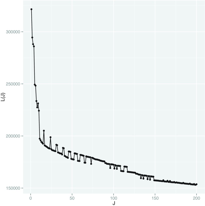
with (Appendix Fig. 1). Algorithm 2 applies this idea to choose a list of candidate values up to the square root of total number of instances.

Appendix FIG. 1.

A graphical interpretation of the conjugacy between and J. We use the K-means initialization to compute surrogate values for for a large collection of . The value that can yield J clusters in the global solution must satisfy When satisfies this condition, a line with slope passing through on the graph should be tangent to the trace of all values. Although using the surrogate values can lead to the curve connecting the values to be non-convex, making the solution for not hold for some J, we can use a convex approximation to the trace of so that a exists for each J. A simpler approach is to order from largest to smallest and requires the following condition for . . Algorithm 2 essentially applies this idea to select the values. Each J corresponds to a of value that satisfies the conjugacy inequality. The algorithm essentially tries to identify the range of that leads up to number of clusters.

Algorithm 2:

Algorithm for choosing m candidate values.

1. Compute the surrogate values of for .

2. Let for .

3. Choose -th, -th, -th quantile in the as candidate values.

4. Given a selected , choose the initial number of clusters as .

Finally, we use the Silhouette score (Rousseeuw, 1987), which has been successfully used for evaluating goodness of fit in clustering, across these values of the tuning parameters.

3. Results

3.1. Computational experiments

We designed computational experiments to evaluate MAD-Bayes MBASIC in settings where the underlying truth is known. In our experiments, we considered I user-specified loci (e.g., promoters from I genes, binding sites of a TF, or peaks from a ChIP-seq experiment). Given multiple simulated ChIP-seq data sets, there are different “baseline” methods for performing these loci-focused analyses. Therefore, in addition to MBASIC, we considered such alternative approaches that practitioners might adopt.

• − MBASIC: The EM algorithm on the full MBASIC model, where singleton, that is, unclusterable, loci are also taken into account.

• − SE-HC: A two-stage method with first state estimation on individual data sets (i.e., conventional peak calling), and then combining the results by hierarchical clustering on the posterior probabilities of the states from the first stage.

• − SE-MC: A two-stage method with first state estimation on individual data sets (i.e., conventional peak calling), and then combining the results by mixture clustering on the binarized results , where from the first stage.

• − PE-MC: A two-stage method with first parameter estimation on individual data sets to determine the state-specific observation distributions (e.g., distributions of the read counts), and then combining the results by simultaneous state inference and mixture clustering. This is essentially similar to MBASIC, except that state-specific densities are fixed and not updated at every iteration.

The alternatives to MBASIC use two-stage procedures for model estimation, decoupling either the estimation of the state-space variables or the distributional parameters from the mixture modeling of state-space clustering. For example, SE-HC corresponds to overlapping user-specified loci with the peak sets from the ENCODE project and generating and clustering the binary overlap or peak confidence profiles of the loci. In contrast, PE-MC is analogous to estimating the distributional parameters of state-space for each individual experiment separately and then clustering with these fixed distributions as in Wei et al. (2012) and Zeng et al. (2013). These benchmark algorithms are in spirit analogous to procedures in many applied genomic data analyses, where the association between observational units is estimated separately from the estimation of individual data set-specific parameters (Gerstein et al., 2012; Wei et al., 2012; Wei et al., 2015).

For the MAD-Bayes algorithm, we evaluated all the three clustering initializations: Adaptive K-means, K-means, and K-means++. The MAD-Bayes algorithm automatically selects the number of clusters. We used the Silhouette score for SE-HC to accommodate hierarchical clustering and used Bayesian Information Criterion for the other methods. The experiments utilized I = 4000 genomic loci, clusters, and experimental conditions. For each condition, the number of replicates, n_k, was drawn from 1 to 3 with probabilities . The clustering concentration parameter was simulated from noninformative prior . The state probabilities, 's, were simulated from . The Log-normal parameters were set as follows: the mean was simulated from , where s represented the state label, and the standard error was set to . We considered four scenarios by varying the number of states S between 2 and 4, and the proportion of singleton loci as . Here, singletons represented loci with overall ChIP-seq enrichment profile different than the clusters, that is, unclusterable locus, and introduced noise to the model. Results for each setting were summarized over 10 simulated data sets. We compared the algorithms in terms of run time, state-space inference (identifying whether or not each locus is bound), and also the clustering structure through the adjusted Rand index (Rand, 1971).

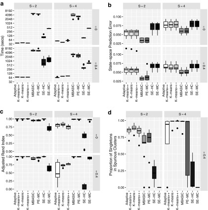
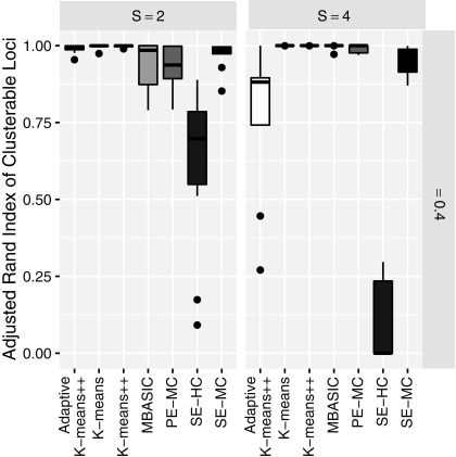
Figure 2a displays run-time comparisons of the methods and indicates that all three implementations of the MAD-Bayes algorithm are about 100 times faster than the EM on full MBASIC and the PE-MC algorithm, and about 10 times faster than the two-step SE-HC and SE-MC algorithms. This speed improvement is significant and makes it possible for the MBASIC framework to scale up. For example, MAD-Bayes algorithm can process and (e.g., DNase accessible regions in the genome across all the available ENCODE ChIP-seq data) in about 6 hours, whereas the EM algorithm on full MBASIC requires more than a week.

FIG. 2.

(a) Run-time comparisons on a 64 bit machine with Intel Xeon 3.0 GHz processor and 64GB of RAM and eight cores. (b) State-space prediction error. (c) Clustering accuracy based on the adjusted Rand index. (d) Clustering assignments of the singletons when

We also observe that speedup in run time does not come at a significant loss in accuracy. Figure 2b compares state-space prediction errors of the algorithms and indicates that although MAD-Bayes MBASIC does not perform as accurately as the EM algorithm on full MBASIC and PE-MC, it performs significantly better than SE-HC and SE-MC algorithms, both of which would be the baseline choices for many practitioners. Existence of singleton genomic loci deteriorates performance of all the algorithms. When there are no singletons, MAD-Bayes algorithm with varying cluster initializations performs the best (Fig. 2c). When indicating that genomic loci do not belong to any cluster, the MAD-Bayes algorithm tends to generate extra, that is, spurious, clusters for such loci (Fig. 2d) instead of forcing them into other clusters. As a result, the true clusters are largely preserved and less polluted by singletons (Appendix Fig. 2) compared with other methods that do not handle singletons (PE-MC, SE-HC, SE-MC).

Appendix FIG. 2.

Comparison of the clustering accuracy with the adjusted Rand index by excluding the singleton loci.

3.2. Application to histone ChIP-seq data from GM12878 cells

The key inference question for the MBASIC framework is identifying the enrichment patterns for a given set of user-specified loci across large sets of ChIP-seq data sets and grouping these loci to elucidate similarities and differences. From this point of view, the MBASIC framework is more loci-focused and not directly comparable with any of the available joint analysis methods that can handle large data sets. However, to get a general sense of how MBASIC would compare with ChromHMM (Ernst and Kellis, 2010) and its computationally efficient version Spectacle (Song and Chen, 2015), we analyzed ChIP-seq data of eight histone marks (H3k4me1, H3k4me2, H3k4me3, H3k9ac, H3k27ac, H3k27me3, H3k36me3, and H4k20me1 from GM12878 cells) from the ENCODE project. Raw data and peak calls for these marks are available at (www.encodeproject.org). We used the 9038 peaks on chr 18 from the ENCODE uniform processing pipeline as the input loci to MAD-Bayes MBASIC and fixed the number of clusters as 20 because Spectacle identified robust number of chromatin states across multiple chromatin modification data sets as 20. As a result, we also set the number of emission states in chromHMM as 20.

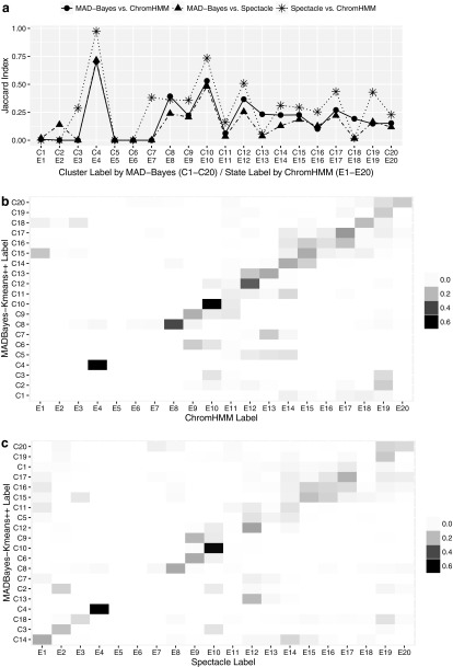
We then performed pairwise comparisons of all the three approaches by matching their clusters/states through maximizing the sum of Jaccard index (Tan et al., 2005).

We reordered the cluster/state labels of MAD-Bayes and Spectacle according to their agreement with ChromHMM. For example, MAD-Bayes cluster “C1” and Spectacle emission state “E1” are both matched to ChromHMM emission state “E1”; however, this does not necessarily indicate that these two are the best matches between MAD-Bayes and Spectacle.

Figure 3a displays that the overall agreements between MAD-Bayes and Spectacle and between MAD-Bayes and ChromHMM follow the same trend with the degree of agreement between Spectacle and ChromHMM, which we think of as the baseline agreement because they are both HMM based. In particular, for the emission states with agreement between Spectacle and ChromHMM, the corresponding MAD-Bayes clusters also have higher agreement with these. When there is large discrepancy between Spectacle and ChromHMM, the MAD-Bayes clusters tend to agree with results from one of the methods. For example, MAD-Bayes “C2” agrees better with Spectacle, and MAD-Bayes “C18” overlaps better with ChromHMM. Figure 3b, c displays comparisons of MAD-Bayes MBASIC with ChromHMM and Spectacle, respectively. We observe that some of MAD-Bayes clusters are distributed over multiple clusters of ChromHMM and Spectacle, for example, MAD-Bayes cluster “C5” overlaps with “E12,” “E13,” and “E14” of both ChromHMM and Spectacle. This overall agreement indicates that the clustering task of MAD-Bayes on the histone marks is reasonable even though it is using selected loci and is not accounting for local dependencies inherent among genomic loci with broad histone marks.

FIG. 3.

(a) Comparison of clusters and state labels between MAD-Bayes, Spectacle, and ChromHMM. (b) Jaccard index between MAD-Bayes clusters and ChromHMM states. (c) Jaccard index between MAD-Bayes clusters and Spectacle states. The diagonal blocks indicate agreement between clusters and states; MAD-Bayes clusters and Spectacle states are ordered according to their overlap with the ChromHMM states. MAD-Bayes, MAP-based asymptotic derivations from Bayes.

4. Discussion

In this article, we derived a MAD-Bayes algorithm by developing a Bayesian version of the MBASIC model. Our evaluations indicated that MAD-Bayes MBASIC significantly improves the computational time without sacrificing accuracy.

We also observed that even though MAD-Bayes MBASIC does not have a built-in mechanism for singletons (unclusterable loci), it groups singletons as additional clusters and minimizes their effect on other more coherent clusters.

We developed MAD-Bayes MBASIC as a fast method for querying large sets (1000s) of ChIP-seq data with user-specified large sets of loci. This represents the first application of the MAD-Bayes framework in a large-scale genome regulation context. From a practical point of view, we showed that this approach is both more efficient and powerful than using individual analysis of each data set and clustering them with an off-the-shelf method such as hierarchical clustering or finite mixture models. From an algorithmic point of view, we developed an empirical method for selecting tuning parameters. This improves the current state of the art for MAD-Bayes implementations because they lack principled methods for tuning parameter selection.

The MBASIC framework offers flexibility in a number of aspects of experimental design, such as different number of replicates under individual experimental conditions. This is a relatively important point because many peak callers will operate separately on individual peaks sets or handle two jointly (Landt et al., 2012), leaving the reconciliation of peaks over multiple replicates to the user. Our current derivation of the MAD-Bayes algorithm relied on Log-normal distribution; however, it can be extended to a larger class of exponential family distributions through the Bregman divergence (Banerjee, 2005). Such extensions are likely to foster its use with other genomic data types such as RNA-seq, DNAse-seq, and methyl-seq, where both state-space estimation and clustering of similar loci pose significant challenges.

Acknowledgments

This work was supported by U01 Grant HG007019 and R01 Grant HG003747 from National Institutes of Health/National Human Genome Research Institute and Center for Predictive Computational Phenotyping.

Author Disclosure Statement

No competing financial interests exist.

References

- Aldous D.J. 1983. Exchangeability and related topics, 1–198. In École d'Été de Probabilités de Saint-Flour XIII 1983. Ed: Hennequin P.L. Springer, Berlin; Heidelberg [Google Scholar]
- Banerjee A. 2005. Clustering with Bregman divergences. J. Mach. Learn. Res. 6, 1705–1749 [Google Scholar]
- Bao Y., Vinciotti V., Wit E., et al. 2013. Accounting for immunoprecipitation efficiencies in the statistical analysis of ChIP-seq data. BMC Bioinformatics 14, 169. [DOI] [PMC free article] [PubMed] [Google Scholar]
- Bao Y., Vinciotti V., Wit E., et al. 2014. Joint modeling of ChIP-seq data via a Markov random field model. Biostatistics 15, 296–310 [DOI] [PubMed] [Google Scholar]
- Bardet A.F., He Q., Zeitlinger J., and Stark A. 2012. A computational pipeline for comparative chip-seq analyses. Nat. Protoc. 7, 45–61 [DOI] [PubMed] [Google Scholar]
- Blackwell D., and MacQueen JB. 1973. Ferguson distributions via polya urn schemes. Ann. Statist. 1, 353–355 [Google Scholar]
- Broderick T., Kulis B., and Jordan M.I. 2013. MAD-Bayes: MAP-based asymptotic derivations from Bayes. In Proceedings of the 30th International Conference on Machine Learning Pgs. 226–234 [Google Scholar]
- Chen K.B., Hardison R., and Zhang Y. 2014. dCaP: Detecting differential binding events in multiple conditions and proteins. BMC Genomics 15, 1–14 [DOI] [PMC free article] [PubMed] [Google Scholar]
- Dempster A., Laird N., and Rubin D. 1977. Maximum likelihood from incomplete data via the EM algorithm. J. Roy. Stat. Soc. B Met. 39, 1–38 [Google Scholar]
- Ernst J., and Kellis M. 2010. Discovery and characterization of chromatin states for systematic annotation of the human genome. Nat. Biotechnol. 28, 817–825 [DOI] [PMC free article] [PubMed] [Google Scholar]
- Ferguson J.P., Cho J.H., and Zhao H. 2012. A new approach for the joint analysis of multiple ChIP-seq libraries with application to histone modification. Stat. Appl. Genet. Mol. Biol. 11, Article 1 [DOI] [PMC free article] [PubMed] [Google Scholar]
- Gerstein M.B., Kundaje A., Hariharan M., et al. 2012. Architecture of the human regulatory network derived from ENCODE data. Nature 489, 91–100 [DOI] [PMC free article] [PubMed] [Google Scholar]
- Hewitt K.J., Kim D.H., Devadas P., et al. 2015. Hematopoietic signaling mechanism revealed from a stem/progenitor cell cistrome. Mol. Cell 59, 62–74 [DOI] [PMC free article] [PubMed] [Google Scholar]
- Hoffman M.M., Buske O.J., Wang J., et al. 2012. Unsupervised pattern discovery in human chromatin structure through genomic segmentation. Nat. Methods 9, 473–476 [DOI] [PMC free article] [PubMed] [Google Scholar]
- Ji H., Li X., Wang Q-F., et al. 2013. Differential principal component analysis of ChIP-seq. Proc. Natl. Acad. Sci. U. S. A. 110, 6789–6794 [DOI] [PMC free article] [PubMed] [Google Scholar]
- Johnson K.D., Hsu A., Ryu M.-J., et al. 2012. Cis-element mutation in a GATA-2-dependent immunodeficiency syndrome governs hematopoiesis and vascular integrity. J. Clin. Invest. 10, 3692–3704 [DOI] [PMC free article] [PubMed] [Google Scholar]
- Kuan P.F., Chung D., Pan G., et al. 2011. A statistical framework for the analysis of ChIP-Seq data. J. Am. Stat. Assoc. 106, 891–903 [DOI] [PMC free article] [PubMed] [Google Scholar]
- Landt S.G., Marinov G.K., Kundaje A., et al. 2012. Chip-seq guidelines and practices of the encode and modencode consortia. Genome Res. 22, 1813–1831 [DOI] [PMC free article] [PubMed] [Google Scholar]
- Liang K., and Keleş S. 2012. Detecting differential binding of transcription factors with ChIPseq. Bioinformatics 28, 121–122 [DOI] [PMC free article] [PubMed] [Google Scholar]
- Mahony S., Edwards M.D., Mazzoni E.O., et al. 2014. An integrated model of multiple-condition ChIP-Seq data reveals predeterminants of Cdx2 binding. PLoS Comput. Biol. 10, e1003501. [DOI] [PMC free article] [PubMed] [Google Scholar]
- Rand W.M. 1971. Objective criteria for the evaluation of clustering methods. J. Am. Stat. Assoc. 66, 846–850 [Google Scholar]
- Roadmap Epigenomics Consortium. 2015. Integrative analysis of 111 reference human epigenomes. Nature 518, 317–330 [DOI] [PMC free article] [PubMed] [Google Scholar]
- Rousseeuw P.J. 1987. Silhouettes: A graphical aid to the interpretation and validation of cluster analysis. J. Comput. Appl. Math. 20, 53–65 [Google Scholar]
- Sohn K-A., Ho J.W.K., Djordjevic D., et al. 2015. hiHMM: Bayesian non-parametric joint inference of chromatin state maps. Bioinformatics 31, 2066–2074 [DOI] [PMC free article] [PubMed] [Google Scholar]
- Song J., and Chen K.C. 2015. Spectacle: Fast chromatin state annotation using spectral learning. Genome Biol. 16, 33. [DOI] [PMC free article] [PubMed] [Google Scholar]
- Song Q., and Smith A.D. 2011. Identifying dispersed epigenomic domains from ChIP-Seq data. Bioinformatics 27, 870–871 [DOI] [PMC free article] [PubMed] [Google Scholar]
- Tan P-N., Steinbach M., and Kumar V. 2005. Chap 8: Cluster analysis: Basic concepts and algorithms. In Introduction to Data Mining. Pearson-Addison-Wesley, Boston [Google Scholar]
- Taslim C., Huang T., and Lin S. 2011. DIME: R-package for identifying differential ChIP-seq based on an ensemble of mixture models. Bioinformatics 27, 1569–1570 [DOI] [PMC free article] [PubMed] [Google Scholar]
- The ENCODE Project Consortium. 2012. An integrated encyclopedia of DNA elements in the human genome. Nature 489, 57–74 [DOI] [PMC free article] [PubMed] [Google Scholar]
- Wei Y., Li X., Wang Q-F., et al. 2012. iASeq: Integrative analysis of allele-specificity of protein-DNA interactions in multiple ChIP-seq datasets. BMC Genomics 13, 681. [DOI] [PMC free article] [PubMed] [Google Scholar]
- Wei Y., Tenzen T., and Ji H. 2015. Joint analysis of differential gene expression in multiple studies using correlation motifs. Biostatistics 16, 31–46 [DOI] [PMC free article] [PubMed] [Google Scholar]
- Zeng X., Sanalkumar R., Bresnick E.H., et al. 2013. jMOSAiCS: Joint analysis of multiple ChIP-seq datasets. Genome Biol. 14, R38. [DOI] [PMC free article] [PubMed] [Google Scholar]
- Zuo C., Chen K., Hewitt K.J., et al. (2016). A hierarchical framework for statespace matrix inference and clustering. Ann. Appl. Stat. In press [DOI] [PMC free article] [PubMed] [Google Scholar]
- Zuo C., and Keleş S. 2014. A statistical framework for power calculations in ChIP-seq experiments. Bioinformatics 30, 853–860 [DOI] [PMC free article] [PubMed] [Google Scholar]