Impact of community disadvantage and air pollution burden on geographic disparities of ovarian cancer survival in California

Abstract

Ovarian cancer survival varies geographically throughout California. The objective of this study is to determine the impact of living in disadvantaged communities on spatial patterns of survival disparities. Including a bivariate spatial smooth of geographic location within the Cox proportional hazard models is an effective approach for spatial analyses of cancer survival. Women diagnosed with advanced Stage IIIC/IV epithelial ovarian cancer (1996–2006) were identified from the California Cancer Registry. The impact of living in disadvantaged communities, as measured by the California Office of Environmental Health Hazard Assessment cumulative CalEnviroScreen 2.0 score, on geographic disparities in survival was assessed while controlling for age, tumor characteristics, quality of care, and race. Community-level air quality indicators and socioeconomic status (SES) were also independently examined in secondary analyses. The Cox proportional hazard spatial methods are available in the MapGAM package implemented in R. An increase in the community disadvantage from the 5^th (less disadvantage) to the 95^th percentile (more disadvantage) was significantly associated with poorer ovarian cancer survival (hazard ratio [HR], 1.16; 95% confidence interval [CI], 1.07–1.26). Ozone levels and SES were the most influential indicators on geographic disparities that warrant further investigation. The use of a bivariate smoother of location within the survival model allows for more advanced spatial analyses for exploring potential air quality-related predictors of geographic disparities.

1.1 Introduction

Each year, an estimated 22,280 women in the United States are diagnosed with ovarian cancer (1). Accounting for over 14,000 cancer-related deaths annually, ovarian cancer is the most fatal of the gynecological cancers (2, 3). Despite the high case fatality, survival rates among women in the general U.S. population have gradually increased throughout the years. As of 2011, 46% of American women diagnosed with this malignancy survive at least 5 years, a significant improvement from the 36% observed 40 years ago (2). However, improved survival is not equitable across all populations. Disparities in ovarian cancer outcomes have been linked to race (4–9), insurance (10) and socioeconomic status (SES) (5), access to quality ovarian cancer care (5, 6, 11, 12), and characteristics of treatment center and physician (13, 14). Receiving appropriate disease-specific care that is adherent to the National Comprehensive Cancer Network (NCCN) treatment guidelines has prevailed as a significant prognostic factor of disease mortality (5, 6). However, many studies have reported that women of Black race, of lower SES and those living in disadvantaged communities are significantly less likely to receive standard cancer-specific care (9, 12, 15, 16). Geographic location has been independently linked to disease-specific survival, and regional differences can only be partially explained by discrepancies in practice patterns and treatment paradigm (6,16–19).

Many factors can contribute to community disadvantage including environmental conditions. Limited research has explored the impact of pollution burden on ovarian cancer survival. In Spain, Lope et al. identified significant disease-specific mortality differences by municipality, which remained independently predictive of survival even after controlling for demographic and treatment variables (19). The authors proposed occupational and environmental exposures as viable explanations of the disparity in mortality distribution observed. A Taiwanese ecological study examining whether an association existed between overall ambient air quality and ovarian cancer mortality revealed a significant relationship between exposure to particulate matter less than 2.5 microns (PM_2.5) and increased risk of death from ovarian cancer (20). Furthermore, the recent findings of significantly shortened lung cancer survival related to air pollutants exposure affirm the need for additional research examining air pollution burden as a possible determinant in ovarian cancer survival (21).

Given that regional variations have previously been noted in California and survival disparities were not completely explained by individual-level multifactorial determinants (16), studying the potential role of the community environment is a critical next step. The objective of the present study is to examine geographic disparities in ovarian cancer survival in California using a Cox proportional hazards additive models, which is an extension of the generalized additive model (GAM) that can systematically determine predictors of the spatial patterns. Our primary aim is to identify whether geographic disparities in survival are related to overall community disadvantage, as measured by the California Office of Environmental Health Hazard Assessment (OEHHA) cumulative CalEnviroScreen (CES) score.

The CES score is comprised of nineteen population and environmental indicators, including community-level air pollution indicators for ozone, PM_2.5, and diesel particulate matter. If results of our analyses suggest community disadvantage is associated with geographic survival disparities, secondary analyses will explore the contributions of these air pollution components to the overall impact of CES score. We selected ozone, PM_2.5, and diesel particulate matter for further investigation if warranted based on the existing literature that predominantly identifies air pollutants as potential risk factors for ovarian cancer survival which are known to affect communities disproportionately. These spatial analyses are a useful tool for exploring potential air quality-related predictors of geographic disparities and generating new hypotheses that would warrant future research in relation to cancer survival.

2.0 Materials and Methods

2.1 Study Population

We investigated the relationship between location at diagnosis, community disadvantage and air pollution burden, and survival among women diagnosed with International Federation of Gynecology and Obstetrics (FIGO) stage IIIC/IV ovarian cancer using data from the California Cancer Registry in a retrospective population-based spatial analysis. Registry case reporting throughout the state is nearly complete (99%) and over 95% of the cases are successfully followed (6). Cases ≥ 18 years of age were ascertained from January 1996 through December 2006 for the entire state. At the time of diagnosis, the median age for the 11,765 study participants was 65.0 years and 7216 women (61.3%) had stage IIIC disease. Only 5342 women (45.4%) received care adherent to NCCN treatment guidelines. Study participants have been described in detail elsewhere (6). The outcome of interest is ovarian cancer–specific survival, defined as the time between diagnosis and death from ovarian cancer or the date of last follow-up. Cases were followed through the end of 2007. The registry collects demographic and tumor characteristics including age at diagnosis, tumor characteristics, insurance type, race, SES, and the latitude and longitude of each subject’s location, represented by the centroid of the address census block.

Community disadvantage and air pollution burden data were obtained from the CalEnviroScreen 2.0 tool developed by OEHHA as part of CalEPA’s environmental justice program (22) and linked to participant addresses at time of diagnosis using ArcMap (version 10.3, ESRI; Redlands, CA). The CalEnviroScreen 2.0 tool was updated in 2014 and calculates a community disadvantage score (CES Score) based on the single assessment of the weighted contribution of nineteen individual indicators related to pollution burden and population characteristics at the census tract level. Twelve of these indicators inform pollution burden, with seven that characterize environmental exposures and five that denote environmental effects. The population characteristics component is comprised of seven indicators. More information about the indicators can be found at the OEHHA CalEnviroScreen Indicators Overview webpage (https://oehha.ca.gov/calenviroscreen/indicators). Our primary objective was to examine the effect of the overall CES score. In secondary exploratory analyses, we were also interested in assessing the contribution of certain individual indicators used to calculate the score, specifically community-level air quality data, on geographic disparities in ovarian cancer survival, controlling for patient, tumor, and treatment characteristics.

Among the indicators used to determine community disadvantage, ambient ozone concentrations, PM_2.5 concentrations, and diesel particulate matter emissions specifically assess community air pollution burden. For these three indicators, the tool uses data obtained from the California Air Resources Board. Integrating estimates from neighboring air monitoring stations using ordinary kriging, data for both PM_2.5 and ozone were estimated at the center of the census tract. Ozone concentration, measured in parts per million (ppm), is calculated as the maximum amount of ozone in an 8-hour period per day that is over the 8-hour state standard of 0.07 ppm. These daily excess concentrations are then averaged over three years (2009–2011) to create one community ozone value for every census tract (23). For PM_2.5, the CalEnviroScreen 2.0 uses the average of the annual means in micrograms per cubic meter (μg/m³) for the same three-year period. For the diesel particulate matter emissions indicators, estimates are obtained from a single summer day in the month of July. This value is the weighted sum of both on-road and non-road emissions obtained from emission models and proxy sources for a 4km by 4km grid, measured in kilograms per day (kg/d). Additional information about the CalEnviroScreen 2.0 tool is available on the OEHHA website (23).

2.2 Spatial Analyses

The geographic survival analyses employ the framework of bivariate spatial smoothing within the Cox proportional hazard models, with simultaneous adjustment for confounders including patient and disease-related prognostic variables (16). The effect of patients’ longitude and latitude of their diagnosis address on survival was modeled using a locally weighted regression (loess) smoother with an a priori optimal span size of 0.3, which was determined by minimizing Akaike information criterion (AIC) (24). The loess smoother adapts to changes in population density while maintaining the Cox proportional hazard model framework, an advantage of this method for cancer registry-based spatial analyses. The span corresponds to the proportion of the data points used for smoothing so that a span of 0.3 uses 30% of the data to fit the local regression. A large span (0.95) results in less spatial variability while a smaller span (0.05) results in more variability (24). Spans ranging from 0.05 to 0.95 and 0.05 increments are evaluated to determine which is optimal. GAM estimation for the bivariate spatial smoother was carried out via backfitting on the linear predictor from the Cox model, using a smoothed Fisher information matrix (25). The fitted spatial Cox model was then used to predict the log hazard multiplier, and the hazard ratio was calculated with the median log hazard for the study area as the reference. A prediction grid of approximately 13,000 5-km cells was used to create maps of continuous hazard ratios (HR) throughout California. Precision for the spatial estimates was calculated using the variance-covariance matrix of the spatial smooth term, and results include maps of the lower and upper confidence HR surfaces. Adjusted HR and 95% confidence intervals (CI) were generated for air pollution burden indicators for an increase from the 5^th to 95^th percentile. Statistical analyses and mapping were conducted in the R Package 3.3.0 (Vienna, Austria) using the MapGAM library (26). Our study cohort includes group-level covariates, which may induce clustering due to spatially correlated factors. To account for this, we sampled one case per census block using the sampcont function in the MapGAM library and then fit the models to the independent survival data using inverse probability weighting (26).

We were interested in assessing the contribution of community disadvantage and air pollution burden to geographic disparities in survival among women diagnosed with ovarian cancer in California (1996–2006). To do this, we first conducted a spatial analysis controlling for age, FIGO stage, grade, histology, tumor size, and insurance type at time of diagnosis, as well as race and adherence to NCCN quality care, to determine geographic patterns of survival that could not be explained by patient, tumor and treatment characteristics. Insurance type, a proxy measure for individual-level SES, was grouped into 6 categories: Managed Care (managed care, HMO, PPO, other private insurance), Medicare, Medicaid, Other Insurance (military, county-funded), Not Insured (self-pay), and Unknown. We then added the following continuous community-level variables in separate models: CES Score (our community disadvantage measure), diesel particulate matter (kg/d), ozone levels (ppm above the standard of 0.07ppm), and PM_2.5 (μg/m3). Variables that did not change the underlying risk pattern by >10% were not included in the final model. Lastly, we included community-level SES in the final model, classified by quintile of Yost score, to disentangle the contribution of environmental and economic factors. The Yost score is a composite block group SES indicator provided by the CA Cancer Registry for all cancer cases that integrates seven socioeconomic data variables available in the U.S. Census including proportion living below the 200% poverty level, median household income, median house value, median rent, education, percent employed and percent blue-collar workers (27). Our current work was reviewed and approved by all relevant Institutional Review Boards.

3.0 Results

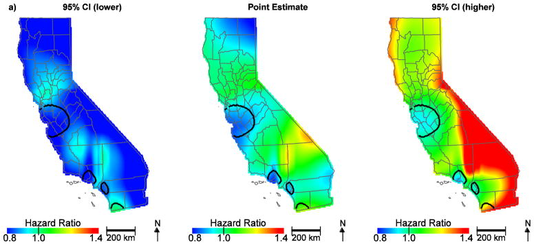
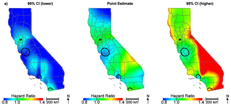
Among the 11,765 patients in our analysis, 38% survived until the end of the study period and the mean ovarian cancer-specific survival for all patients was 27.4 months. After controlling for patient, tumor, and treatment characteristics, we observed significant areas of low hazard ratios in the San Francisco Bay area, Los Angeles and Orange Counties, and increased hazard ratios in San Bernardino County and near the San Diego County/Mexico border (Figure 1a). These patterns suggest that NCCN adherent care is not the only predictor of geographic disparities. The hazard ratios for the effect of location on survival ranged from 0.79 to 1.33. When community disadvantage (as measured by the CES Score) was included in the model, hazard ratios in San Bernardino county were attenuated and no longer significant (Figure 1b, Table 1). The hazard ratio for an increase in the community disadvantage from the 5^th (less disadvantage) to the 95^th percentile (more disadvantage) was 1.16 (95% CI, 1.07–1.26).

Figure 1.

Geographic patterns of ovarian cancer survival adjusted for patient, tumor, and treatment characteristics (a) and further adjusted for community disadvantage (b). Black lines indicate where hazard ratios exclude one.

Table 1.

Hazard Ratios and 95% Confidence Intervals for Predictors in Spatial Analyses

Predictor	HR (95% CI)
CalEnvironScreen Tool Variables
Community Disadvantage (CES Score)a	1.16 (1.07, 1.26)
Diesela (kg/d)	1.03 (0.97, 1.10)
Ozonea (ppm)	1.14 (1.07, 1.26)
PM2.5a (μg/m3)	1.10 (1.01, 1.19)
SES
Lowest	1.24 (1.14, 1.36)
Low-Middle	1.19 (1.11, 1.28)
Middle	1.15 (1.07, 1.23)
High-Middle	1.08 (1.01, 1.16)
Highest	referent
Insurance Type
Medicare	1.00 (0.95, 1.06)
Medicaid	1.06 (0.97, 1.17)
Other insurance	0.94 (0.86, 1.03)
Uninsured	1.07 (0.92, 1.25)
Unknown	1.08 (0.94, 1.23)
Managed care	referent
Race
Black	1.19 (1.07, 1.33)
Hispanic	0.93 (0.86, 1.00)
Asian/Pacific Islander	0.93 (0.85, 1.01)
White	referent
Stage
Stage IIIC	referent
Stage IV	1.52 (1.44, 1.59)
Grade
Grade 1	0.62 (0.52, 0.73)
Grade 2	0.90 (0.83, 0.97)
Grade 3	Referent
Grade 4	1.03 (0.95, 1.12)
Unknown	1.29 (1.22, 1.36)
Histology
Serous	referent
Clear cell	1.44 (1.25, 1.66)
Endometrioid	0.87 (0.78, 0.98)
Mucinous	1.56 (1.38, 1.77)
Adenocarcinoma NOS*	1.46 (1.37, 1.57)
Other	1.24 (1.17, 1.32)
NCCN Guidelines
Non-adherent	1.26 (1.20, 1.32)
Adherent	referent
Age	1.02 (1.02, 1.03)

Abbreviations: CI, confidence interval; HR, hazard ratio; SES, socioeconomic status.

^aHazard ratios are presented for an increase from the 5^th to the 95^th percentile.

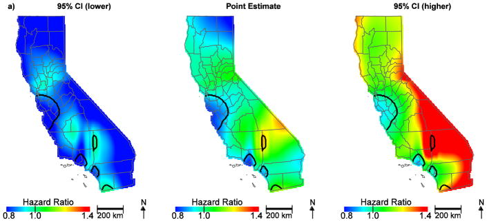
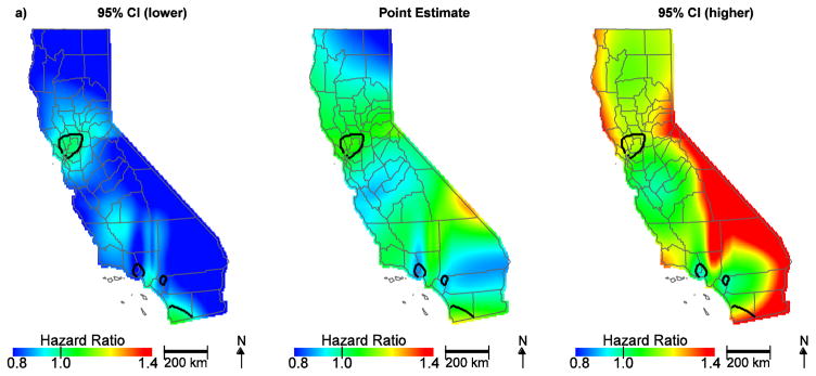
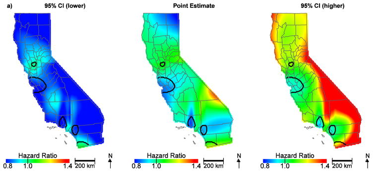
To further assess the individual factors contributing to community disadvantage, air quality indicators and SES at the community level were also evaluated. Table 2 shows the distribution of community air quality burden by SES classified per increasing quintile. While the CalEnviroScreen 2.0 tool indicator for community diesel PM was not an important predictor (HR, 1.03; 95% CI, 0.97–1.10; Figure 2a), the CalEnviroScreen 2.0 tool indicator for ozone (HR, 1.14; 95% CI, 1.07–1.26), PM_2.5 (HR, 1.10; 95% CI, 1.01–1.19) and the Yost SES measure (lowest HR, 1.24; 95% CI, 1.14–1.36; low-middle HR, 1.19; 95% CI, 1.11–1.28; middle HR, 1.15; 95% CI, 1.07–1.23; high-middle HR, 1.08; 95% CI, 1.01–1.16) contributed to geographic disparities in ovarian cancer survival (Figure 2b, Table 1). Notably, hazard ratios in the San Francisco Bay area are no longer protective. This is largely due to ozone, which is lower along the coast; adding ozone to the model and predicting at the median value changes the HR to approximately one and reveals a significant area of slightly increased HR approaching the central valley (Figure 3a). Further, when we control for SES, the protective HRs in Orange County are attenuated and no longer significant, indicating the importance of economic factors in survival in this region (Figure 3b). Overall, accounting for community air quality indicators and SES reduces the geographic variation in ovarian cancer survival and attenuates the magnitude of HRs throughout the state, but significant areas of increased and decreased HRs still exist.

Table 2.

Distribution of Air Quality Indicators by SES Quintile Among 11,765 Women with Ovarian Cancer

		Ozone (ppm)		PM2.5 (ug/m3)		Diesel PM (kg/d)
SES Quintile	N (%)	Median	5th–95th Range	Median	5th–95th Range	Median	5th–95th Range
Lowest	1528 (13.0)	0.026	0 – 0.727	11.76	5.04 –14.85	18.90	1.30 –67.76
Low-Middle	2137 (18.1)	0.029	0 – 0.598	10.23	4.62 –13.87	14.67	0.54 –43.58
Middle	2481 (21.1)	0.022	0 – 0.509	9.36	5.05 –13.62	12.61	0.52 –39.12
High-Middle	2751 (23.4)	0.009	0 – 0.432	9.07	5.35 –13.19	12.49	1.14 –36.73
High	2868 (24.4)	0.003	0 – 0.265	8.83	6.30 –12.49	10.89	1.54 –35.45

Figure 2.

Geographic patterns of ovarian cancer survival adjusted for diesel PM (a) compared to ozone, PM_2.5, and SES (b), in addition to patient, tumor, and treatment characteristics. Black lines indicate where hazard ratios exclude one.

Figure 3.

Geographic patterns of ovarian cancer survival adjusted for ozone (a) and SES, (b), in addition to patient, tumor, and treatment characteristics. Black lines indicate where hazard ratios exclude one.

4.0 Conclusion

Our analyses suggest that ovarian cancer survival disparities exist among California women depending on where they live, and these disparities may be related to community disadvantage. Adding CES Score to the spatial model attenuated hazard ratios in San Bernardino county, suggesting that other factors including pollution and/or socioeconomic burden are contributing to poor survival outcomes in that region. To our knowledge, this study is the first to explore the impact of community-level air pollution burden on geographic differences in ovarian cancer survival accounting for spatial confounding by individual-level patient, tumor and treatment characteristics. While patient age and receiving standard care are leading predictors of ovarian cancer survival, SES, ozone and PM_2.5 levels may be also contributing factors to the geographic variation in different regions of California. These exploratory results indicate that further work is needed to understand their independent and combined effects at both the individual and community levels (28, 29). Despite these patterns, geographic differences in ovarian cancer survival persisted, suggesting that other environmental or social indicators may also be contributing to observed disparities.

Our survival analyses incorporated a smooth term for location within the Cox proportional hazard models to measure spatial variability. This approach is useful for assessing important predictors of geographic disparities in cancer survival, providing simultaneous adjustment for confounders, and disentangling the contribution of spatially variable risk factors to observed patterns. The CalEnviroScreen 2.0 tool allowed for screening of community disadvantage and air pollution burden as potential predictors that could warrant further investigation. Spatial limitations of this study include the availability of only address at diagnosis and group-level exposure measures. Although the multi-level analysis is accounted for in the spatial methods applied, ideally we would like to have robust measures of air pollution burden and SES at both an individual and community level. While patient characteristics, including insurance type, were available at the individual-level from the cancer registry, SES was based on census block group-level data, and environmental indicators from the CalEnviroScreen 2.0 tool were measured at the census tract level. When using community-level measures, choosing the most appropriate geographic scale is not always obvious, as community has a range of connotations, and adds to the potential for misclassification of community-level SES and pollution burden resulting from the modifiable areal unit problem (30).

Individual level exposures, especially those that consider activity patterns, would be useful for simultaneously examining individual- and community-level factors. Furthermore, air monitors are sparse in parts of the state with low population density, so exposure estimates for those cases would be less reliable. Cases may have moved after diagnosis, which may result in exposure misclassification as well. The California Cancer Registry does not currently have residential histories for cases. The analyses were also limited temporally as the air monitoring data were only available for a single three-year time period. That said, our analyses are suggestive of a potential association between ovarian cancer survival and community disadvantage, independent of SES, quality of care received, and other important predictors. In addition, based on exploratory analyses of community-level air quality measures, further analyses of air pollution and ovarian cancer survival are warranted.

Highlights.

• Geographic location disproportionately affects ovarian cancer survival in disadvantaged communities with higher air pollution burdens.

• Women living in geographic areas of California with low community-level SES and high ozone levels have poorer ovarian cancer survival.

• The use of a bivariate spatial smoother within the Cox proportional hazard model allows for more advanced geospatial analyses.

References

- 1.Siegel RL, Miller KD, Jemal A. Cancer statistics. CA Cancer J Clin. 2016;66:7–30. doi: 10.3322/caac.21332. [DOI] [PubMed] [Google Scholar]
- 2.SEER Cancer Statistics Factsheets: Ovary Cancer. National Cancer Institute; [Accessed on November 4, 2016]. http://seer.cancer.gov/statfacts/html/ovary.html. [Google Scholar]
- 3.Moyer VA. Screening for ovarian cancer: U.S. Preventive Services Task Force reaffirmation recommendation statement. Ann Intern Med. 2012;157:900–904. doi: 10.7326/0003-4819-157-11-201212040-00539. [DOI] [PubMed] [Google Scholar]
- 4.Zeng C, Wen W, Morgans AK, Pao W, Shu X-O, Zheng W. Disparities by Race, Age, and Sex in the Improvement of Survival for Major Cancers: Results From the National Cancer Institute Surveillance, Epidemiology, and End Results (SEER) Program in the United States, 1990 to 2010. JAMA Oncol. 2015;1:88–96. doi: 10.1001/jamaoncol.2014.161. [DOI] [PMC free article] [PubMed] [Google Scholar]
- 5.Bristow RE, Powell MA, Al-Hammadi N, Chen L, Miller JP, Roland PY, et al. Disparities in ovarian cancer care quality and survival according to race and socioeconomic status. J Natl Cancer Inst. 2013;105:823–832. doi: 10.1093/jnci/djt065. [DOI] [PMC free article] [PubMed] [Google Scholar]
- 6.Bristow RE, Chang J, Ziogas A, Anton-Culver H, Vieira VM. Spatial analysis of adherence to treatment guidelines for advanced-stage ovarian cancer and the impact of race and socioeconomic status. Gynecol Oncol. 2014;134:60–67. doi: 10.1016/j.ygyno.2014.03.561. [DOI] [PMC free article] [PubMed] [Google Scholar]
- 7.Jelovac D, Armstrong DK. Recent progress in the diagnosis and treatment of ovarian cancer. CA Cancer J Clin. 2011;61:183–203. doi: 10.3322/caac.20113. [DOI] [PMC free article] [PubMed] [Google Scholar]
- 8.Terplan M, Schluterman N, McNamara EJ, Tracy JK, Temkin SM. Have racial disparities in ovarian cancer increased over time? An analysis of SEER data. Gynecol Oncol. 2012;125:19–24. doi: 10.1016/j.ygyno.2011.11.025. [DOI] [PubMed] [Google Scholar]
- 9.Brewer KC, Peterson CE, Davis FG, Hoskins K, Pauls H, Joslin CE. The influence of neighborhood socioeconomic status and race on survival from ovarian cancer: A population-based analysis of Cook County, Illinois. Ann Epidemiol. 2015;25:556–563. doi: 10.1016/j.annepidem.2015.03.021. [DOI] [PMC free article] [PubMed] [Google Scholar]
- 10.Harlan LC, Clegg LX, Trimble EL. Trends in surgery and chemotherapy for women diagnosed with ovarian cancer in the United States. J Clin Oncol. 2003;21:3488–3494. doi: 10.1200/JCO.2003.01.061. [DOI] [PubMed] [Google Scholar]
- 11.Farley JH, Tian C, Rose GS, Brown CL, Birrer M, Maxwell GL. Race does not impact outcome for advanced ovarian cancer patients treated with cisplatin/paclitaxel: an analysis of Gynecologic Oncology Group trials. Cancer. 2009;115:4210–4217. doi: 10.1002/cncr.24482. [DOI] [PMC free article] [PubMed] [Google Scholar]
- 12.Peterson CE, Rauscher GH, Johnson TP, Kirschner CV, Freels S, Barrett RE, et al. The effect of neighborhood disadvantage on the racial disparity in ovarian cancer-specific survival in a large hospital-based study in Cook County, Illinois. Front Public Health. 2015;3:8. doi: 10.3389/fpubh.2015.00008. [DOI] [PMC free article] [PubMed] [Google Scholar]
- 13.Bristow RE, Zahurak ML, Diaz-Montes TP, Giuntoli RL, Armstrong DK. Impact of surgeon and hospital ovarian cancer surgical case volume on in-hospital mortality and related short-term outcomes. Gynecol Oncol. 2009;115:334–338. doi: 10.1016/j.ygyno.2009.08.025. [DOI] [PubMed] [Google Scholar]
- 14.Bristow RE, Palis BE, Chi DS, Cliby WA. The National Cancer Database report on advanced-stage epithelial ovarian cancer: Impact of hospital surgical case volume on overall survival and surgical treatment paradigm. Gynecol Oncol. 2010;118:262–267. doi: 10.1016/j.ygyno.2010.05.025. [DOI] [PubMed] [Google Scholar]
- 15.Long B, Chang J, Ziogas A, Tewari KS, Anton-Culver H, Bristow RE. Impact of race, socioeconomic status, and the health care system on the treatment of advanced-stage ovarian cancer in California. Am J Obstet Gynecol. 2014;133:156–157. doi: 10.1016/j.ajog.2014.10.1104. [DOI] [PubMed] [Google Scholar]
- 16.Bristow RE, Chang J, Ziogas A, Gillen DL, Bai L, Vieira VM. Spatial analysis of advanced-stage ovarian cancer mortality in California. Am J Obstet Gynecol. 2015;213:43, e1–8. doi: 10.1016/j.ajog.2015.01.045. [DOI] [PMC free article] [PubMed] [Google Scholar]
- 17.Dehaeck U, McGahan CE, Santos JL, Carey MS, Swenerton KD, Kwon JS. The impact of geographic variations in treatment on outcomes in ovarian cancer. Int J Gynecol Cancer. 2013;23:282–287. doi: 10.1097/IGC.0b013e31827b87b1. [DOI] [PubMed] [Google Scholar]
- 18.Fairfield KM, Lee Lucas F, Earle CC, Small L, Trimble EL, Warren JL. Regional variation in cancer-directed surgery and mortality among women with epithelial ovarian cancer in the Medicare population. Cancer. 2010;116:4840–4848. doi: 10.1002/cncr.25242. [DOI] [PubMed] [Google Scholar]
- 19.Lope V, Pollán M, Pérez-Gómez B, Aragonés N, Vidal E, Gómez-Barroso D, et al. Municipal distribution of ovarian cancer mortality in Spain. BMC Cancer. 2008;8:258. doi: 10.1186/1471-2407-8-258. [DOI] [PMC free article] [PubMed] [Google Scholar]
- 20.Hung L-J, Chan T-F, Wu C-H, Chiu H-F, Yang C-Y. Traffic air pollution and risk of death from ovarian cancer in Taiwan: fine particulate matter (PM2. 5) as a proxy marker. J Toxicol Environ Health A. 2012;75:174–182. doi: 10.1080/15287394.2012.641200. [DOI] [PubMed] [Google Scholar]
- 21.Eckel SP, Cockburn M, Shu Y-H, Deng H, Lurmann FW, Liu L, et al. Air pollution affects lung cancer survival. Thorax. 2016;71:891–8. doi: 10.1136/thoraxjnl-2015-207927. [DOI] [PMC free article] [PubMed] [Google Scholar]
- 22.August LM, Faust JB, Cushing L, Zeise L, Alexeeff GV. Methodological considerations in screening for cumulative environmental health impacts: Lessons learned from a pilot study in California. Int J Environ Res Public Health. 2012;9:3069–3084. doi: 10.3390/ijerph9093069. [DOI] [PMC free article] [PubMed] [Google Scholar]
- 23.CalEnviroScreen. [Accessed on Januay 10, 2016];Office of Environmental Health Hazard Assessment (OEHHA) http://oehha.ca.gov/calenviroscreen/maps-data/download-data.
- 24.Vieira V, Webster T, Weinberg J, Aschengrau A, Ozonoff D. Spatial analysis of lung, colorectal, and breast cancer on Cape Cod: an application of generalized additive models to case-control data. Environ Health. 2005;4:11. doi: 10.1186/1476-069X-4-11. [DOI] [PMC free article] [PubMed] [Google Scholar]
- 25.Adaptive Statistical Methods for the Analysis of Sequential and Spatial Observation Data [dissertation] Irvine, CA: University of California, Irvine; 2016. [Google Scholar]
- 26.Vieira VM, Bartell SM, Bliss RL. MapGAM: Mapping Smoothed Odds Ratios from Individual-Level Data, R package, version 1.0. 2016. [Google Scholar]
- 27.Yost K, Perkins C, Cohen R, Morris C, Wright W. Socioeconomic status and breast cancer incidence in California for different race/ethnic groups. Cancer Causes Control. 2001;12:703–11. doi: 10.1023/a:1011240019516. [DOI] [PubMed] [Google Scholar]
- 28.Krieger N, Chen JT, Waterman PD, Rehkoph DH, Subramanian SV. Race/ethnicity, gender, and monitoring socioeconomic gradients in health: a comparison of area-based socioeconomic measures—the Public Health Disparities Geocoding Project. Am J Public Health. 2003;93:1655–1671. doi: 10.2105/ajph.93.10.1655. [DOI] [PMC free article] [PubMed] [Google Scholar]
- 29.Krieger N, Chen JT, Waterman PD, Soobader M-J, Subramanian SV, Carson R. Geocoding and monitoring of US socioeconomic inequalities in mortality and cancer incidence: does the choice of area-based measure and geographic level matter? Am J Epidemiol. 2002;156:471–482. doi: 10.1093/aje/kwf068. [DOI] [PubMed] [Google Scholar]
- 30.Openshaw S. The Modifiable Areal Unit Problem. Geobooks; Norwich, England: 1984. [Google Scholar]