An Advanced Deep Learning Approach for Ki-67 Stained Hotspot Detection and Proliferation Rate Scoring for Prognostic Evaluation of Breast Cancer

Abstract

Being a non-histone protein, Ki-67 is one of the essential biomarkers for the immunohistochemical assessment of proliferation rate in breast cancer screening and grading. The Ki-67 signature is always sensitive to radiotherapy and chemotherapy. Due to random morphological, color and intensity variations of cell nuclei (immunopositive and immunonegative), manual/subjective assessment of Ki-67 scoring is error-prone and time-consuming. Hence, several machine learning approaches have been reported; nevertheless, none of them had worked on deep learning based hotspots detection and proliferation scoring. In this article, we suggest an advanced deep learning model for computerized recognition of candidate hotspots and subsequent proliferation rate scoring by quantifying Ki-67 appearance in breast cancer immunohistochemical images. Unlike existing Ki-67 scoring techniques, our methodology uses Gamma mixture model (GMM) with Expectation-Maximization for seed point detection and patch selection and deep learning, comprises with decision layer, for hotspots detection and proliferation scoring. Experimental results provide 93% precision, 0.88% recall and 0.91% F-score value. The model performance has also been compared with the pathologists’ manual annotations and recently published articles. In future, the proposed deep learning framework will be highly reliable and beneficial to the junior and senior pathologists for fast and efficient Ki-67 scoring.

Introduction

Automated breast cancer (BC) detection research has been increased nowadays due to the inflation of BC mortality rate worldwide¹. In the GLOBOCAN 2012, BC has been reported as the second most common cancer, which occurs mostly among women than men^{2, 3}. As per the Nottingham grading system, BC grading is done based on the scores of nuclear pleomorphism, mitotic count, and tubule formation⁴. Additionally, to confirm the BC subtypes, to distinguish normal and malignant tumor and to guide treatment decisions smoothly, immunohistochemical (IHC) analysis of breast tissue is required. The most commonly used IHC markers are Ki-67, estrogen receptors, progesterone receptor, protein P53 and human epidermal growth factor-2⁵.

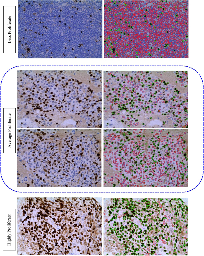
Ki-67, non-histone protein, is one of the essential prognostic and predictive markers for BC detection. Gerdes et al.^{6, 7} reported that Ki-67 signature is exhibit only in proliferating cells and disappears in quiescent cells. Furthermore, the Ki-67 expression doesn’t appear in G0 cell cycle but instead appears in G1, S, G2, M cell cycle⁷. The level of Ki-67 becomes low during G1 and S cell cycle phase but increases during mitosis (exception anaphase and telophase). Mitotic index is considered as one of the most significant proliferation markers for BC grading or screening. Although it has some limitations, e.g., the rate of mitosis proliferation is non-linearly related to the number of mitosis in high power field⁸. Hence, the IHC analysis of Ki-67 using monoclonal antibody has emerged for the alternative assessment for the proliferation index⁹. The proliferation score determines the severity of BC as follows: low (<15%), average (16–30%) and highly (>31%) proliferate⁵. Patients with high Ki-67 is very sensitive to radiotherapy and chemotherapy¹⁰. Ki-67 expression possesses the significant predictive and prognostic value in BC. Personalized treatment and diagnosis facility can improve the survival rates of BC patients. Hence, the identification of accurate grading (grade I, grade II and grade III) remains always a challenge for pathologists. Till now, the clinical decision on BC grading is mostly made manually based on both predictive and prognostic pathological markers. The manual assessment of Ki-67 is subjective, error-prone and dependent on the Intra and inter-observer ambiguities. Moreover, in the rural and urban areas with minimum or few advanced instrumentation, manual inspection of Ki-67 scoring may provide wrong results. Henceforth, automated assessment of Ki-67 scoring is highly required. The automatic scoring will provide high throughput, more objective and reproducible results in comparison with the manual evaluation. The proliferation score is calculated as the ratio between total numbers of immunopositive nuclei and a total number of nuclei present in the image¹¹. The immunopositive (brown color) and immunonegative (blue color) nuclei together called as hotspots. Figure 1 shows the Ki-67 stained BC images according to their proliferation score and their corresponding color distribution map using open source ImageJ software. To date, the Ki-67 automated assessment was done mainly based on conventional imaging techniques. But due to the heterogeneous and massive dataset in medical imaging or biomedical applications scientists are getting interested in deep learning. Deep learning is a versatile biomedical research tool with numerous potential applications. P. Mamoshina et al. (2016) proposed a deep learning framework in biomedicine application¹². Y. Xu et al. (2014) reported deep learning for medical image analysis¹³. This paper has been structured as an introduction, literature review, experimental setup, results & discussion and finally conclusion.

Figure 1.

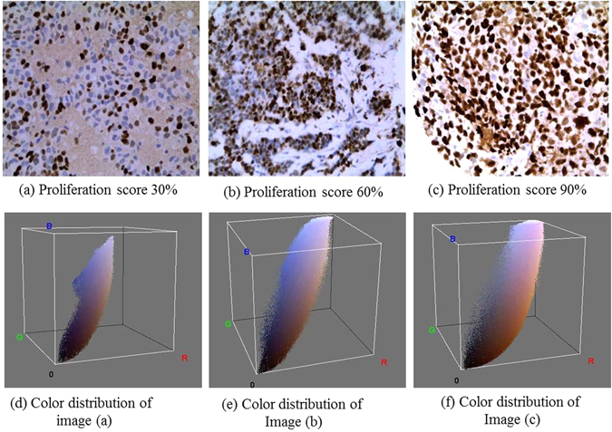
Ki-67 proliferation scoring by the pathologists with respect to differential color distribution: Three input Ki-67 stained images of breast cancer at 40× with the scores (a) = 30%; (b) = 60%; (c) = 90%; and color spectrum visualization of the inputs images (d–f).

Literature review

Many machine learning techniques have been published for Ki-67 scoring using IHC stained BC images. To the best of our knowledge, most of the Ki-67 scoring methods are based on conventional machine learning techniques. Based on the extensive literature survey, we conclude that there are no such reports available till date specially aimed to the deep learning approaches for considering much finer information inherent in the microscopic images. Table 1 shows the characterization of different Ki-67 scoring methods.

Table 1.

Characterization of Ki-67 scoring approaches.

Categories	Year	Cancer type	Methodology used	Results
Conventional techniques	2016	Nasopharyngeal cancer	K-means clustering	91.8% Segmentation accuracy15
	2015	Meningiomas and Oligodendrogliomas tumor	Morphology operation, thresholding, feature extraction and classification	The results shows the effectiveness of the proposed algorithm33
	2014	Neuroendocrine tumor	Learning based approach	89% precision, 91% recall, 90% F-score11
	2014	Breast Cancer	Otsu thresholding	High correlation observed between manual and automated procedure34
	2014	Breast cancer	Aperio Genie and Nuclear v9 software	Misclassification rate 5–7%35
	2013	Pancreatic neuroendocrine tumor	Voting-Based Seed Detection, Repulsive Deformable Model, Two step classification	87.68% classification accuracy, 88.01% sensitivity and 87.12% specificity36
	2013	Rabbit Liver	Inform 1.4 image analysis software	Useful in clinical practice37
	2012	Breast cancer	K-means clustering	T-test shows reliable proliferation rate38
	2012	Not mentioned	Watershed segmentation, Laplacian-of-Gaussian filtering, SVM classifier	90% sensitivity at confidence level I, 99% sensitivity at confidence level VIII39
	2012	Breast Cancer	Slidepath Tissue IA system software	Excellent agreement between manual and automated technique40
	2010	Breast cancer	ImmunoRatio software	20% labeling index as a cutoff, 2.2 hazard ratio41
	2009	Meningiomas tumor	Thresholding, watershed and morphological operations, SVM classifier	The proposed method helpful for further research42
Deep Learning	No work has been carried out for Ki-67 scoring using deep learning approaches

Review on conventional techniques

M. Abubakar et al.¹⁴ proposed a computer vision algorithm for Ki-67 scoring in BC tissue microarray images. Their algorithm shows promising performance measure in comparison with other scoring technique. The authors achieved 90% classification accuracy with 0.64 kappa value. The automated quantification of Ki-67 using nasopharyngeal carcinoma has been described in P. Shi et al.¹⁵. Their algorithm mainly consists of smoothing, decomposition, feature extraction, K-means clustering, and quantification. They achieve 91.8% segmentation accuracy. F. Zhong et al. (2016) compared the visual and automated Ki-67 scoring on BC images¹⁶. The authors used total 155 Ki-67 immunostained slides of invasive BC. The scoring has been performed based on hotspots and average score. They employed correlation coefficient to analyze the consistency and to minimize the errors between the two techniques. Z. Swiderska et al.¹⁷ employed computer vision algorithm for hotspots selection from the whole slide meningioma images. The authors used color channel selection, Otsu thresholding, morphological filtering, feature selection and classification. The authors achieved high correlation between manual and automated hotspots detection. F. Xing et al. (2014) proposed an automated machine learning algorithm for Ki-67 counting and scoring using neuroendocrine tumor images¹¹. The proposed algorithm has three stages. Stage-I comprises of seed point detection, segmentation, feature extraction and cell level probability measurement. Stage-II consists of tumor or non-tumor cell classification, probability map generation, and feature extraction. Finally, stage-III provide immunopositive and negative cell classification along with Ki-67 scoring. This approach achieved 89% precision, 91% recall and 90% F-score. J. Konsti et al.¹⁸ reported virtual application for Ki-67 assessment in BC. The algorithm mainly developed using ImageJ software. At first, images were processed using color deconvolution to separate hematoxylin and diaminobenzidine stain color channels. Then a mask was moved over the images to get target objects. This approach showed 87% agreement and 0.57 kappa value. The Ki-67 scoring using Gamma-Gaussian Mixture Model (GGMM) has not been attempted yet. Khan et al. (2012) proposed GMM model for mitosis identification from histopathological images¹⁹.

Review on deep learning techniques

To the best of our knowledge, automatic Ki-67 scoring and hotspots detection using deep learning approach were not attempted yet.

The major contributions of this paper include:

• Development of an advanced deep learning model for Ki-67 stained hotspots detection and calculation of proliferation index.

• Inclusion of decision layer in the proposed deep learning framework.

• It is a value addition in terms of main quantification in the already existing established techniques for Ki-67 scoring.

Experimental setup

Slide preparation and image acquisition

The slide having histological sections of the tissue biopsy was stained by using Ki-67 monoclonal antibody. At 40x magnification, total 450 microscopic images from 90 (histologically confirmed) slides were grabbed and digitally stored using Zeiss Axio Imager M2 microscope with Axiocam ICc5 camera at constant contrast and brightness in BioMedical Imaging Informatics (BMI) Lab of School of Medical Science & Technology, IIT Kharagpur and Department of pathology, Tata Medical Center (TMC), Kolkata. The field of view (FOV) of the each image-matrix was 2048 × 1536 pixels (width × height). All the images contained almost 259,884 (131,053 immunopositive and 128,831 immunonegative) annotated and un-annotated nuclei. All procedures, e.g. slide preparation, image acquisition, etc. were performed in accordance with the institutional guidelines. The ethical statement details have been discussed in Ethics and consent statements.

Layers of Convolutional Network (CN)

A CN mainly consists of multiple consecutive convolution layers, subsampling/pooling layers, non-linear layers and fully-connected layers. Let, f is a CN and a composition of a sequence of N number of layers or functions (f ₁, f ₂…f _N). The mapping between input (w) and output (u) vector of a CN can be represented as²⁰:

$$u=f(w;X_1,X_2,X_3,\dots ,X_N)=f_1(w;X_1)\circ f_2(.;X_2)\dots \circ f_{N-1}(.;X_{N-1})\circ f_N(.;X_N)$$ 1

Conventionally, f _N has been assigned to perform convolution or, non-linear activation or, spatial pooling. Where X _N denotes the bias and weight vector for the N ^th layer f _N. Given a set of η training data ${\{(w^{(i)},u^{(i)})\}}_{i=1}^{\eta }$, we can estimate the vectors (X ₁, X ₂, X ₃, …, X _N) as follows

$$\underset{X_1,X_2,X_3,\dots ,X_N}{\text{arg}\min }\frac{1}{\eta }{\sum }_{i=1}^{\eta }{f}_{Loss}(f(w^{(i)};X_1,X_2,X_3,\dots ,X_N),u^{(i)})$$ 2

where f _LOSS indicates loss function. The equation 2 can be performed using stochastic gradient descent and backpropagation methods.

Convolution layers

In deep learning, the convolution operation extracts different low-level (e.g. lines, edges, and corner) and higher-level hierarchical features from the input images. In our proposed deep learning framework multiple layers are stacked in a way so that the input of h ^th layer will be the output of (h−1)^th layer. A convolutional layer usually learns convolutional filters to calculate feature map. The equation²¹ of feature map ($F{M}_m^h$) at a level m will be

$$F{M}_m^h=f({\alpha }_m^h+\sum _{j}F{M}_j^{h-1}\times G_{jm}^h)$$ 3

In equation 3, $j\in [0,\sum _{j}F{M}_{in}^{h-1}-1]$ represents input feature map indices and $m\in [0,\sum _{j}F{M}_{out}^h-1]$ denotes output feature map indices. Here, $F{M}_{in}^{h-1}$ and $F{M}_{out}^h$ represent a number of input and output feature maps at h ^th level. $G_{jm}^h$ and ${\alpha }_m^h$ represent biases and corresponding kernels respectively. In each convolution layer, there are two components which create feature maps. The first element is Local Receptive Field and the second part is shared weights. A feature map is the output of one filter applied to the previous layer. The each unit in a feature map looks for the same feature but at different positions of the input image.

Max-pooling layer

The pooling layers have been employed to get spatial invariance by reducing the feature maps’ resolution. The pooling operation makes the features more robust against distortion and noise. There are two types of pooling mostly used in deep learning. Those are average pooling and max-pooling. In both the cases, the input is divided into two-dimensional spaces (non-overlapping). Based on our requirement and image characteristics we have chosen max-pooling operations in our proposed framework. The advantages of this type of layer are the capability of downsampling the input image size and create positive invariance over the local regions. The max-pooling function has been calculated using the below equation^{22, 23}.

$${\mathrm{\Psi }}_j=\max ({\psi }_i^{n\times n}z(n,n))$$ 4

The max-pooling window can be overlapped and arbitrary size. Here ψ is the input image, z denotes window function and n × n = 71 × 71 is the input patch size.

Rectified Linear Unit

In deep learning, Rectified Linear Units (ReLUs) have been used as an activation function and as a gradient descent vector. It is defined by the below equation^{24, 25}

$$q(r)=\max (0,r)$$ 5

where q denotes model’s output function with an input r. The size of input and output of this layer is same. The ReLU enhances the performance of the network without disturbing receptive fields and increases nonlinearity of the decision function. ReLU trains the CN much faster than the other existing non-linear functions (e.g., sigmoid, hyperbolic tangent and absolute of hyperbolic tangent).

Fully Connected (FC) Layer

The FC layer is often used as a final layer of a CN in a classification problem. This layer mathematically sums a weighting of features of a previous layer. It works like a classifier. This layer is not spatially located and serves as a simple vector. In the proposed model, FC layer height and width of each blob is set to 1.

Dropout Layer

Dropout is a regularization technique which is mostly used for reducing overfitting and preventing complex-co-adaptions on training data. Due to this layer, the learned weights of nodes become more insensitive to the weights of the other nodes. This layer helps to increase the accuracy of the model by switching off the unnecessary nodes in the existing network. The dropout neurons do not contribute in the backpropagation and forward pass.

Decision Layer

An additional decision layer comprises of decision trees, has been introduced in the proposed deep learning framework. As per our knowledge, the concept of decision layer in deep learning framework has not been used so far. The inclusion of decision layer increases the performance of the proposed model. In our proposed method we used decision trees inspired by P. Kontschieder et al.²⁶. The proposed decision layer consists of decision nodes and prediction nodes. The decision layer algorithm is a recursive algorithm and implemented in C++²⁷. The column of the blob data table has been split based on information gain or least entropy.

Let, the input and finite output spaces are denoted by X and Y respectively. In the decision tree, decision nodes are also called internal nodes of the tree and indexed by D. Similarly, prediction nodes are called terminal nodes and indicated by P. Each decision node 0 ∈ D assigned a decision function $f_d(.;\mathrm{\Theta }):X\to [0,1]$. Each projection node p ∈ P possesses probability distribution π _p over Y. When a sample x ∈ X reaches a decision node d it will send to the right or left subtree based on the output of $f_d(x;\mathrm{\Theta })$. On decision trees f _d are binary, and the routine is deterministic. The final prediction result for sample x from tree T with decision notes parametrized by Θ is denoted by

$$P_T[y|x,\mathrm{\Theta },\pi ]={\sum }_{p\in P}{\pi }_{py}{\mu }_p(x|\mathrm{\Theta })$$ 6

Here, π _py and π = (π _p)p ∈ P represents the probability of a sample reaching leaf p on class y and routine function indicated by ${\mu }_p(x|\mathrm{\Theta })$. When x ∈ X, $\sum _p{\mu }_p(x|\mathrm{\Theta })=1$.

In decision nodes decision function works based on stochastic routine and is defined as

$$f_d(x;\mathrm{\Theta })=\sigma (f_r(x;\mathrm{\Theta }))$$ 7

Here σ(x) is a sigmoid function and defined as $\sigma (x)=\frac{1}{(1+e^{-x})}$. The $f_r(.;\mathrm{\Theta }):X\to ℝ$ is a real-valued function. An ensemble of decision trees are called decision forest and are denoted by

$$F=\{T_1,T_2,\dots ,T_z\}$$ 8

The learning of decision trees along with decision nodes and prediction nodes have been done using CAFFE stochastic gradient descent approach. The pictorial representation of decision layer connections in CAFFE has been shown in Fig. 2.

Figure 2.

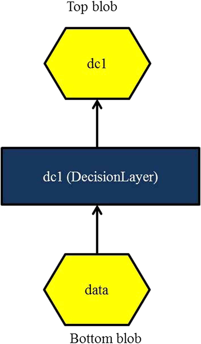
Shows pictorial representation of decision layer connections in CAFFE.

Patch selection

Patch selection is a very much essential part of the proposed methodology. The overall patch selection work flow diagram has been shown in Fig. 3. Due to variations of nuclei size, shape and the localization of nuclei, image patches may vary. In the case of overlapping nuclei, it is very complicated to crop a patch which will only contain a single nucleus (immunopositive or immunonegative). Henceforth, we have detected seed point using Gamma mixture model (GMM) with Expectation-Maximization algorithm. The algorithm is an iterative method and used to find maximum posterior or maximum likelihood. The iteration alternates between performing an expectation (E) and maximization (M) for each parameter.

Figure 3.

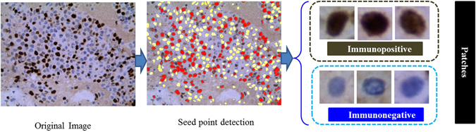
Illustrates the flow diagram of the patch detection from original images.

Let I is an image I = (I ₁, I ₂, I ₃, …, I _Q) where Q represents a number of pixels and I _Q denotes gray-level intensity of a pixel. To infer a configuration of positive labels L, K = (K ₁, K ₂, K ₃, … K _Q) where K _Q ∈ L L = {0, 1}. Now as per MAP criteria the labeling satisfies:

$$K^{⁎}=\underset{k}{\text{arg}\max }\{Y(I|K,\mathrm{\Theta })Y(K)\}$$ 9

Here, Y(K) is a Gibbs distribution. In the Expectation-Maximization algorithm the equation 9 can be written as

$$K^{⁎}=\underset{K\in k}{\text{arg}\max }\{U(I|K,\mathrm{\Theta })+U(K)\}$$ 10

Here, U denotes urinary potential or likelihood energy and denoted by

$$U(I|K,\mathrm{\Theta })={\sum }_Q[\frac{{(I_Q-{\mu }_{KQ})}^2}{2{\sigma }_K^2}+\ln {\sigma }_K]$$ 11

As per the hypothesis, we are assuming that the segmented region’s intensity will follow a Gaussian distribution with parameters σ _xi = (μ _xi, σ _xi). This hypothesis is unable to model real-life objects. So for complex distribution GMM is the best choice for the engineers. A GMM with c components is represented by below equations²⁸:

$${\sigma }_i=\{({\mu }_{i,1},{\sigma }_{i,1},w_{i,1}),\dots ,({\mu }_{i,c},{\sigma }_{i,c},w_{i,c})$$ 12

The Gaussian distribution with parameters can be written as

$$G(z;{\alpha }_i)=\frac{1}{\sqrt{2\pi {\sigma }_i^2}}\exp \left(-\frac{{(z-{\mu }_i)}^2}{2{\sigma }_i^2}\right)$$ 13

Comparing the equation 12 with equation 13, we get the weighted probability as follows

$$G_{mix}(z;{\alpha }_i)={\sum }_{c=1}^h{w}_{i,c}G(z;{\mu }_{i,c},{\sigma }_{i,c})$$ 14

For a color RGB image the pixel intensity is a 3-dimensional vector. The parameters of GMM now becomes²⁸

$${\alpha }_{xi}=({\mu }_{i,1},{\sum }_{i,1},w_{i,1})\dots ({\mu }_{i,c},{\sum }_{i,c},w_{i,c})$$ 15

Comparing equation 15 with equation 11, we will get the likelihood Energy Equation as below

$$U(I|K,\mathrm{\Theta })={\sum }_Q\left[\frac{1}{2}{(I_Q-{\mu }_{KQ})}^T{\sum }_{KQ}^{-1}(I_Q-{\mu }_{KQ})+\ln \left|{\sum }_{KQ}\right|\frac{1}{2}\right]$$ 16

The seed points of immunopositive and immunonegative nuclei have been denoted as red and yellow color respectively. Finally, each patch of size 71 × 71 have been cropped using centroid points of each selected seed points, and lastly, patches have been feed into our proposed deep learning framework.

Proposed Deep Learning Model (DLM)

The proposed DLM has been developed using CAFFE deep learning framework, and CUDA enabled parallel computing platform²⁹. The architectural details of the proposed DLM have been shown in Table 2. The proposed model includes one decision layer, two fully connected layers, four max-pooling layers, five convolution layers and six ReLUs. The decision layer has been added after fifth convolutional layer. ReLU has been employed after each convolutional layer to fasten the computing time. Dropout layer has been inserted after first FC layer to avoid the over-fitting. After the rigorous experiment, it was found that dropout ratio = 0.5 is provided the best result in this dataset. The workflow diagram of the proposed DLM has been illustrated in Fig. 4. Our proposed model learns from the labeled data.

Table 2.

Proposed deep learning approach.

Layer	Type	Maps	Neurons	Filter size
0	Input Image	3	71 × 71	—
1	Conv-1	90	70 × 70	2 × 2
2	MP-1	90	35 × 35	2 × 2
3	Conv-2	180	32 × 32	4 × 4
4	MP-2	180	16 × 16	2 × 2
5	Conv-3	360	14 × 14	3 × 3
6	MP-3	360	7 × 7	2 × 2
7	Conv-4	720	6 × 6	2 × 2
8	MP-4	720	3 × 3	2 × 2
9	Conv-5	1440	2 × 2	2 × 2
10	Decision layer	—	720	1 × 1
11	FC-1	—	100	1 × 1
12	FC-2	—	2	1 × 1

Figure 4.

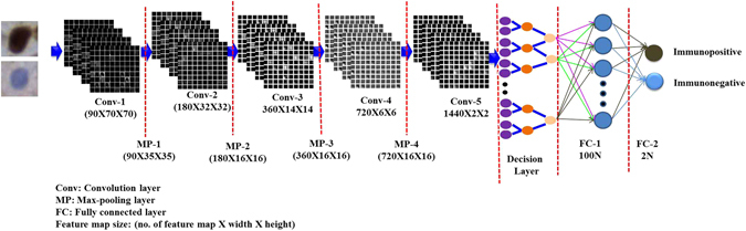
Shows the flow diagram of the proposed deep learning model.

Parameter initialization

The numbers of training and validation samples were considered as 70% and 30% respectively out of 450 images. The training and validation batch size were set to 128. The testing interval and maximum iteration were assigned to 5000 and 450,000 respectively. The other important parameters include learning rate (=0.01), weight decay (=0.005) and momentum (=0.85). The detailed source code of the model and parameter initialization files has been included as supplementary documents.

Ethics and consent statements

Ethical approval has been taken from the TMC, Kolkata (ref. no. EC/GOVT/07/14; dated August 11, 2014) and Indian Institute of Technology, Kharagpur (ref. IIT/SRIC/SAO/2015; dated July 23, 2015) to conduct this research work. The patient consent forms have been signed by the patient and their close relatives. The slides were prepared and maintained by TMC, Kolkata. All procedures, e.g. slide preparation, image acquisition, etc. were performed in accordance with the institutional policies.

Results and Discussion

In this portion, we assess the efficacy of our proposed deep learning framework. We randomly divided the image patch dataset into five subsets (5-fold cross validation); each subset includes 20% of the total data. It should be noted that during training phase each time we performed patch selection, model learning and classification using the four subsets. Finally, the selected patches and trained model were used to assess the performance of the left-out testing sub-dataset. Five-fold cross validation results have been shown in Table 3. Furthermore, performance based on various combinations of training and testing dataset has been indicated in Table 4. The seed point selection and object detection algorithms have been developed using MATLAB and Python tools on a machine with AMD Opteron processor 128 GB RAM, NVIDIA Titan X pascal GPU. The proposed cascaded framework achieved almost 0.974 training accuracy and 0.0945 loss.

Table 3.

5-fold cross-validation.

Cross-Validation	Pr	Re	F-score
1st	0.930	0.881	0.910
2nd	0.927	0.875	0.910
3rd	0.926	0.879	0.920
4th	0.930	0.881	0.900
5th	0.931	0.880	0.910
Average	0.930	0.880	0.910

Table 4.

Performance based on various combinations of training and testing dataset.

Training images (%)	Testing images (%)	Pr	Re	F-score
0	100	0.909	0.777	0.838
25	75	0.925	0.877	0.901
50	50	0.929	0.880	0.904
75	25	0.950	0.882	0.914
100	0	0.971	0.893	0.930

Quantitative evaluation

The quantitative assessment results have been shown in Table 5. Figure 5 illustrates the regression curve (R² = 0.9991) between automatic and manual hotspots detection. The graph indicates that the model generated immunopositive and immunonegative nuclei count provides almost exact results in comparison to the pathologists’ count. The model is evaluated using precision (Pr), recall (Re) and F-score as below³⁰:

$$\mathrm{Pr}(\%)=\frac{\mathrm{True}\mathrm{positive}}{\mathrm{True}\mathrm{positive}+\mathrm{False}\mathrm{negative}}\times 100$$ 17

$$\mathrm{Re}(\%)=\frac{\mathrm{True}\mathrm{positive}}{\mathrm{True}\mathrm{positive}+\mathrm{False}\mathrm{positive}}\times 100$$ 18

$$F(\%)=2\times \left(\frac{\mathrm{Pr}\times \mathrm{Re}}{\mathrm{Pr}+\mathrm{Re}}\right)\times 100$$ 19

Table 5.

Quantitative performance measures for Ki-67 scoring.

Confusion Matrix		Pr	Re	F-score
17028	2277	0.93	0.88	0.91
1287	15840

Figure 5.

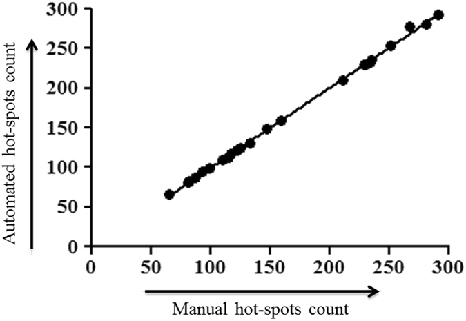
Regression curve between automated and manual hotspots count.

Our proposed model achieved 93% precision, 88% recall and 91% F-score value. We also added confusion matrix for better understanding the results. Figure 6 shows precision and recall curve across 5-fold cross-validation.

Figure 6.

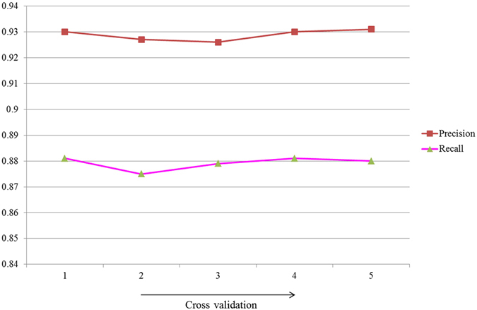
Shows precision and recall curve.

Qualitative evaluation

The first, second, third, fourth and fifth convolution layer feature maps of immunopositive and immunonegative nuclei patches have been displayed in Fig. 7. The feature maps generated by using various kernels in convolution layers decodes the signature of the expression level of color content of brown (for immunopositive) and blue (for immunonegative) nuclei. In this context, Fig. 7 has been revised by presenting two immunopositive and immunonegative images. It can be observed that the ki-67 expression is different with respect to filters for immunopositive and immunonegative nuclei. Basically from the feature maps, we can assume a nucleus is immunopositive or, not. But for the confirmation, we have to classify the image. Due to a clear visualization of feature maps, only a few feature maps in each layer have been displayed. The qualitative and hotspots detection results have been shown in Figs 8 and 9 respectively. Hence, we can conclude that our proposed methodology is performing better than the existing ones.

Figure 7.

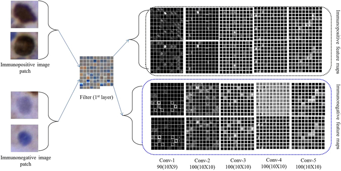
Visualization of feature maps of various convolution layers.

Figure 8.

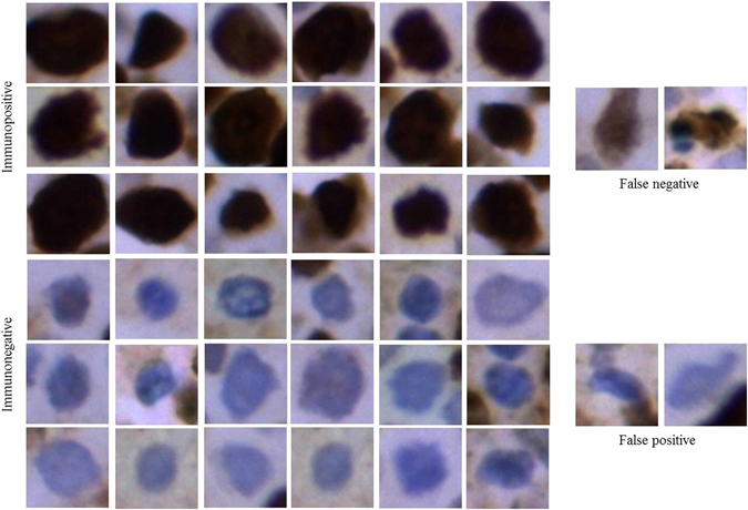
Ki-67 detection results by using the proposed algorithm.

Figure 9.

Overall detection of hotspots in breast cancer IHC images at different proliferation levels.

Computational time

Computation time is one of the most vital factors of machine learning. For this reason, we have always tried to keep the patch size as small as possible. The small patch size decreases the computation time and increases the detection performance. The model took almost 5 days (24 × 5 = 120 hours) for training and, on average, takes 1.33 seconds (in GPU) and 1.64 seconds (in CPU) to detect the hotspots (immunopositive and immunonegative nuclei). In comparison, the method in N. Khan et al.³¹ requires an average of 7 seconds only to segment a color image. Overall, the proposed method is much more efficient than the existing Ki-67 scoring methods.

Automated Ki-67 proliferation scoring (APS)

The automated Ki-67 proliferation scoring has been calculated using the below equation³²

$$APS(\%)=\frac{TIP}{TIP+TIN}\times 100$$ 20

here, the TIP = total number of immunopositive nuclei and the TIN = total number of immunonegative nuclei. Table 6 shows the overall proliferation score based on two pathologists and our automated technique. In this table reference range shows the standard proliferated category and their ranges, which are already gold standard in pathology. We compared the proliferation score of both the pathologists’ with the proposed technique. It is observed that in both the cases error rate is negligible. More specifically, in the less proliferated category error rate is 0.06%, average proliferated category error rate is 0.01% and highly proliferated category error rate is 0%. It can be observed that the proposed deep learning framework provides consistent and efficient results as evident from the similar performance.

Table 6.

Overall proliferation score.

Reference range 26	Pathologists	MPS (%)	APS (%)
Less proliferate (<15%)	Expert-1	12.87	13.00
	Expert-2	13.01	13.00
	Average	12.94	13.00
Average proliferate (16–30%)	Expert-1	27.29	27.99
	Expert-2	28.00	27.99
	Average	27.64	27.99
Highly proliferate (>31%)	Expert-1	90.00	90.00
	Expert-2	90.00	90.00
	Average	90.00	90.00

‘MPS’: Manual Proliferation Score.

The training performance graph has been shown in Fig. 10. After 297,000 iterations the accuracy and loss graph become saturated. Hence we have only shown the graph up to 297,000 iterations. Figure 11 illustrates the ROC curve and the area under the curve (AUC) is 91.

Figure 10.

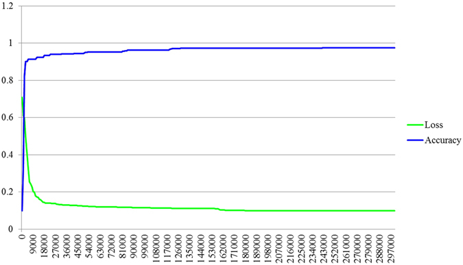
Training performance graph.

Figure 11.

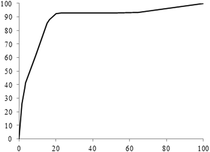
ROC graph for showing the overall performance of the proposed methodology.

Comparison with the existing methods

From the exhaustive literature review, it is evident that the quantification and proliferation rate scoring of Ki-67 stained BC or other cancer images using deep learning approach has not been attempted so far. Moreover, there have few limitations, e.g., nonstandard dataset, conventional imaging approach, etc. for which we cannot directly measure the performances of our proposed method with the existing methodologies. Based on some technical understanding of image similarities, we compared the qualitative and quantitative performances with the two recently published articles^{15, 31} on Ki-67 scoring in Table 7. Furthermore, we measured the efficiency of our proposed framework with other conventional methods. Table 8 shows the comparison of performance measures with various combinations, e.g. proposed method but without decision layer, GMM and random forest but without deep network, GMM plus SVM but without deep network, replacing the decision layer with additional FC layer and the proposed methodology. From the Table 8 it is obvious that proposed method including decision layer provides better performance in terms of precision, recall and F-sore value in comparison with the other techniques. Henceforth, the proposed methodology is far better than the existing methods.

Table 7.

Comparison with the existing methods.

Comparison parameters	P. Shi et al.15	N. Khan et al.31	Proposed Methodology
Image type	Human nasopharyngeal carcinoma Xenografts	Neuroendocrine tumor	Breast cancer
Sample size	100 images	57 images	450 images
Image size	2040 × 1536	10 × 5 K	2048 × 1536
Image Magnification	40x	40x	40x
Methodology used	Conventional techniques (smoothing, color channel decomposition, local feature extraction, K-means, watershed segmentation)	Conventional technique (Perceptual clustering)	Deep Learning integrated with decision layer
Accuracy (%)	91.8	94.60	97
Computation time (sec)	1.7	7	1.33 in GPU and 1.64 in CPU
CPU or GPU used	CPU	CPU	CPU and GPU both
Error rate	0.82	Not mentioned	0.41

Table 8.

Comparison of performance measures.

Conditions	Pr (%)	Re (%)	F-score (%)
Without decision layer	89	80	82
GMM + random forest	91	65	76
GMM + SVM	93	80	86
Replacing decision layer with additional FC layer	87	88	87
Proposed methodology	93	88	91

Conclusion

In this manuscript, our contribution is twofold, (i) development of an efficient deep learning model comprises of decision layer for automated detection of hotspots, and (ii) development of an automatic proliferation rate scoring technique of Ki-67 positively stained BC images. The proposed deep learning model is capable of computing the scoring index with any IHC image, provided that immunopositive nuclei will manifest as brown color and immunonegative nuclei will show as blue color. The proposed framework starts with a seed point detection using GMM which makes the algorithm more robust. This step substantially eliminates unnecessary background objects. Our proposed deep learning model considers both, the pathologist’s information as well as spatial similarity while detecting hotspots. Our quantitative and qualitative evaluation results showed the better performance of our proposed model. The model provides higher learning accuracy and performance scores as measured by precision, recall and F-score, in comparison with the existing conventional techniques for Ki-67 scoring. The model performance has also been compared with the pathologists’ manual annotations. Prospectively, this model will be highly beneficial to the pathologists for fast and efficient Ki-67 scoring from breast IHC (cancer) images.

Author Contributions

M. Saha carried out the whole experiment alone, collected slides from TMC Kolkata, grabbed images and prepared the manuscript. C. Chakraborty supervised the research work and also contributed in reviewing the manuscript. I. Arun, R. Ahmed and S. Chatterjee made slides and provided advice.

Competing Interests

The authors declare that they have no competing interests.

References

- 1.Saha, M. et al. Histogram based thresholding for automated nucleus segmentation using breast imprint cytology. In Advancements of Medical Electronics, 49–57 (Springer, 2015).
- 2.Ferlay J, et al. Cancer incidence and mortality worldwide: sources, methods and major patterns in globocan 2012. International journal of cancer. 2015;136:E359–E386. doi: 10.1002/ijc.29210. [DOI] [PubMed] [Google Scholar]
- 3.Saha M, Mukherjee R, Chakraborty C. Computer-aided diagnosis of breast cancer using cytological images: A systematic review. Tissue and Cell. 2016;48:461–474. doi: 10.1016/j.tice.2016.07.006. [DOI] [PubMed] [Google Scholar]
- 4.Saha M, et al. Quantitative microscopic evaluation of mucin areas and its percentage in mucinous carcinoma of the breast using tissue histological images. Tissue and Cell. 2016;48:265–273. doi: 10.1016/j.tice.2016.02.005. [DOI] [PubMed] [Google Scholar]
- 5.Zaha DC. Significance of immunohistochemistry in breast cancer. World journal of clinical oncology. 2014;5:382. doi: 10.5306/wjco.v5.i3.382. [DOI] [PMC free article] [PubMed] [Google Scholar]
- 6.Gerdes J, Schwab U, Lemke H, Stein H. Production of a mouse monoclonal antibody reactive with a human nuclear antigen associated with cell proliferation. International journal of cancer. 1983;31:13–20. doi: 10.1002/ijc.2910310104. [DOI] [PubMed] [Google Scholar]
- 7.Gerdes J, et al. Cell cycle analysis of a cell proliferation-associated human nuclear antigen defined by the monoclonal antibody ki-67. The Journal of Immunology. 1984;133:1710–1715. [PubMed] [Google Scholar]
- 8.Romero Q, Bendahl P-O, Fernö M, Grabau D, Borgquist S. A novel model for ki67 assessment in breast cancer. Diagnostic pathology. 2014;9:1. doi: 10.1186/1746-1596-9-118. [DOI] [PMC free article] [PubMed] [Google Scholar]
- 9.Thor AD, Liu S, Moore DH, II, Edgerton SM. Comparison of mitotic index, in vitro bromodeoxyuridine labeling, and mib-1 assays to quantitate proliferation in breast cancer. Journal of Clinical Oncology. 1999;17:470–470. doi: 10.1200/JCO.1999.17.2.470. [DOI] [PubMed] [Google Scholar]
- 10.Tewari M, Krishnamurthy A, Shukla HS. Predictive markers of response to neoadjuvant chemotherapy in breast cancer. Surgical oncology. 2008;17:301–311. doi: 10.1016/j.suronc.2008.03.003. [DOI] [PubMed] [Google Scholar]
- 11.Xing F, Su H, Neltner J, Yang L. Automatic ki-67 counting using robust cell detection and online dictionary learning. IEEE Transactions on Biomedical Engineering. 2014;61:859–870. doi: 10.1109/TBME.2013.2291703. [DOI] [PubMed] [Google Scholar]
- 12.Mamoshina, P. et al. Applications of deep learning in biomedicine. Molecular pharmaceutics13(5), 1445–1454 (2016). [DOI] [PubMed]
- 13.Xu, Yan, et al. Deep learning of feature representation with multiple instance learning for medical image analysis. Acoustics, Speech and Signal Processing (ICASSP), 2014 IEEE International Conference on. IEEE, 2014.
- 14.Abubakar, M. et al. High-throughput automated scoring of ki67 in breast cancer tissue microarrays from the breast cancer association consortium. The Journal of Pathology: Clinical Research (2016). [DOI] [PMC free article] [PubMed]
- 15.Shi, P. et al. Automated ki-67 quantification of immunohistochemical staining image of human nasopharyngeal carcinoma xenografts. Scientific Reports 6 (2016). [DOI] [PMC free article] [PubMed]
- 16.Zhong F, et al. A comparison of visual assessment and automated digital image analysis of ki67 labeling index in breast cancer. PloS one. 2016;11:e0150505. doi: 10.1371/journal.pone.0150505. [DOI] [PMC free article] [PubMed] [Google Scholar]
- 17.Swiderska, Z. et al. Comparison of the manual, semiautomatic, and automatic selection and leveling of hot spots in whole slide images for ki-67 quantification in meningiomas. Analytical Cellular Pathology 2015 (2015). [DOI] [PMC free article] [PubMed]
- 18.Konsti J, et al. Development and evaluation of a virtual microscopy application for automated assessment of ki-67 expression in breast cancer. BMC clinical pathology. 2011;11:1. doi: 10.1186/1472-6890-11-3. [DOI] [PMC free article] [PubMed] [Google Scholar]
- 19.Khan, A. M., El-Daly, H., & Rajpoot, N. M. (2012, November). A gamma-gaussian mixture model for detection of mitotic cells in breast cancer histopathology images. In Pattern Recognition (ICPR), 21st International Conference, 149–152 (2012).
- 20.Sirinukunwattana K, et al. Locality sensitive deep learning for detection and classification of nuclei in routine colon cancer histology images. IEEE transactions on medical imaging. 2016;35:1196–1206. doi: 10.1109/TMI.2016.2525803. [DOI] [PubMed] [Google Scholar]
- 21.Xing F, Xie Y, Yang L. An automatic learning-based framework for robust nucleus segmentation. IEEE transactions on medical imaging. 2016;35:550–566. doi: 10.1109/TMI.2015.2481436. [DOI] [PubMed] [Google Scholar]
- 22.Scherer, D., Müller, A. & Behnke, S. Evaluation of pooling operations in convolutional architectures for object recognition. In International Conference on Artificial Neural Networks, 92–101 (Springer, 2010).
- 23.Nagi, J. et al. Max-pooling convolutional neural networks for vision-based hand gesture recognition. In Signal and Image Processing Applications (ICSIPA), 2011 IEEE International Conference on, 342–347 (IEEE, 2011).
- 24.Dahl, G. E., Sainath, T. N. & Hinton, G. E. Improving deep neural networks for lvcsr using rectified linear units and dropout. In 2013 IEEE International Conference on Acoustics, Speech and Signal Processing, 8609–8613 (IEEE, 2013).
- 25.Krizhevsky, A., Sutskever, I. & Hinton, G. E. Imagenet classification with deep convolutional neural networks. In Advances in neural information processing systems, 1097–1105 (2012).
- 26.Kontschieder, P., Fiterau, M., Criminisi, A. & Rota Bulo, S. Deep neural decision forests. In Proceedings of the IEEE International Conference on Computer Vision, 1467–1475 (2015).
- 27.https://github.com/bonz0/Decision-Tree, access on March 31, 2017.
- 28.Wang Q. Gmm-based hidden markov random field for color image and 3d volume segmentation. arXiv preprint arXiv. 2012;1212:4527. [Google Scholar]
- 29.Jia, Y. et al. Caffe: Convolutional architecture for fast feature embedding. In Proceedings of the 22nd ACM international conference on Multimedia, 675–678 (ACM, 2014).
- 30.Xu J, et al. Stacked sparse autoencoder (ssae) for nuclei detection on breast cancer histopathology images. IEEE transactions on medical imaging. 2016;35:119–130. doi: 10.1109/TMI.2015.2458702. [DOI] [PMC free article] [PubMed] [Google Scholar]
- 31.N. Khan MK, Yearsley MM, Zhou X, Frankel WL, Gurcan MN. Perceptual clustering for automatic hotspot detection from ki-67-stained neuroendocrine tumour images. Journal of microscopy. 2014;256:213–225. doi: 10.1111/jmi.12176. [DOI] [PubMed] [Google Scholar]
- 32.Kyzer S, Gordon PH. Determination of proliferative activity in colorectal carcinoma using monoclonal antibody ki67. Diseases of the colon & rectum. 1997;40:322–325. doi: 10.1007/BF02050423. [DOI] [PubMed] [Google Scholar]
- 33.Swiderska, Z., Markiewicz, T., Grala, B. & Slodkowska, J. Hot-spot selection and evaluation methods for whole slice images of meningiomas and oligodendrogliomas. In 2015 37th Annual International Conference of the IEEE Engineering in Medicine and Biology Society (EMBC), 6252–6256 (IEEE, 2015). [DOI] [PubMed]
- 34.Klauschen F, et al. Standardized ki67 diagnostics using automated scoring—clinical validation in the gepartrio breast cancer study. Clinical Cancer Research. 2015;21:3651–3657. doi: 10.1158/1078-0432.CCR-14-1283. [DOI] [PubMed] [Google Scholar]
- 35.Laurinavicius A, et al. A methodology to ensure and improve accuracy of ki67 labelling index estimation by automated digital image analysis in breast cancer tissue. Breast Cancer Research. 2014;16:1. doi: 10.1186/bcr3639. [DOI] [PMC free article] [PubMed] [Google Scholar]
- 36.Xing, F., Su, H. & Yang, L. An integrated framework for automatic ki-67 scoring in pancreatic neuroendocrine tumor. In International Conference on Medical Image Computing and Computer-Assisted Intervention, 436–443 (Springer, 2013). [DOI] [PMC free article] [PubMed]
- 37.Van der Loos CM, et al. Accurate quantitation of ki67-positive proliferating hepatocytes in rabbit liver by a multicolor immunohistochemical (ihc) approach analyzed with automated tissue and cell segmentation software. Journal of Histochemistry & Cytochemistry. 2013;61:11–18. doi: 10.1369/0022155412461154. [DOI] [PMC free article] [PubMed] [Google Scholar]
- 38.Al-Lahham, H. Z., Alomari, R. S., Hiary, H. & Chaudhary, V. Automating proliferation rate estimation from ki-67 histology images. In SPIE Medical Imaging 83152A–83152A (International Society for Optics and Photonics, 2012).
- 39.Akakin, H. C. et al. Automated detection of cells from immunohistochemically-stained tissues: application to ki-67 nuclei staining. In SPIE Medical Imaging, 831503–831503 (International Society for Optics and Photonics, 2012).
- 40.Mohammed Z, et al. Comparison of visual and automated assessment of ki-67 proliferative activity and their impact on outcome in primary operable invasive ductal breast cancer. British journal of cancer. 2012;106:383–388. doi: 10.1038/bjc.2011.569. [DOI] [PMC free article] [PubMed] [Google Scholar]
- 41.Tuominen VJ, Ruotoistenmäki S, Viitanen A, Jumppanen M, Isola J. Immunoratio: a publicly available web application for quantitative image analysis of estrogen receptor (er), progesterone receptor (pr), and ki-67. Breast Cancer Research. 2010;12:1. doi: 10.1186/bcr2615. [DOI] [PMC free article] [PubMed] [Google Scholar]
- 42.Grala B, et al. New automated image analysis method for the assessment of ki-67 labeling index in meningiomas. Folia Histochem Cytobiol. 2009;47:587–592. doi: 10.2478/v10042-008-0098-0. [DOI] [PubMed] [Google Scholar]
Associated Data
This section collects any data citations, data availability statements, or supplementary materials included in this article.
Supplementary Materials
Supplementary source code and installation guide