Reassessment of 20th century global mean sea level rise

Significance

Estimates of global mean sea level (GMSL) before the advent of satellite altimetry vary widely, mainly because of the uneven coverage and limited temporal sampling of tide gauge records, which track local sea level rather than the global mean. Here we introduce an approach that combines recent advances in solid Earth and geoid corrections for individual tide gauges with improved knowledge about their geographical representation of ocean internal variability. Our assessment yields smaller trends before 1990 than previously reported, leading to a larger overall acceleration; identifies three major explanations for differences with previous estimates; and reconciles observational GMSL estimates with the sum of individually modeled contributions from the Coupled Model Intercomparison Project 5 database for the entire 20th century.

Abstract

The rate at which global mean sea level (GMSL) rose during the 20th century is uncertain, with little consensus between various reconstructions that indicate rates of rise ranging from 1.3 to 2 mm⋅y⁻¹. Here we present a 20th-century GMSL reconstruction computed using an area-weighting technique for averaging tide gauge records that both incorporates up-to-date observations of vertical land motion (VLM) and corrections for local geoid changes resulting from ice melting and terrestrial freshwater storage and allows for the identification of possible differences compared with earlier attempts. Our reconstructed GMSL trend of 1.1 ± 0.3 mm⋅y⁻¹ (1σ) before 1990 falls below previous estimates, whereas our estimate of 3.1 ± 1.4 mm⋅y⁻¹ from 1993 to 2012 is consistent with independent estimates from satellite altimetry, leading to overall acceleration larger than previously suggested. This feature is geographically dominated by the Indian Ocean–Southern Pacific region, marking a transition from lower-than-average rates before 1990 toward unprecedented high rates in recent decades. We demonstrate that VLM corrections, area weighting, and our use of a common reference datum for tide gauges may explain the lower rates compared with earlier GMSL estimates in approximately equal proportion. The trends and multidecadal variability of our GMSL curve also compare well to the sum of individual contributions obtained from historical outputs of the Coupled Model Intercomparison Project Phase 5. This, in turn, increases our confidence in process-based projections presented in the Fifth Assessment Report of the Intergovernmental Panel on Climate Change.

Estimates of global mean sea level (GMSL) change before the advent of satellite altimetry (e.g., refs. 1–6) rely on a historical data set of coastal tide gauges with both uneven spatial coverage biased toward the Northern Hemisphere and limited temporal sampling (7) (Fig. S1 A and B). These tide gauges are grounded on land, and are thus affected by the vertical motion of the Earth’s crust, caused both by natural processes [e.g., glacial isostatic adjustment (GIA) after the last deglaciation or tectonic deformations] and by anthropogenic activities (e.g., groundwater depletion and dam building). As pointwise measurements, tide gauges further track local sea levels, which reflect the geographical patterns induced by ocean dynamics and geoid changes in response to mass load redistribution (8). Altogether, these factors hamper our ability to provide a unique 20th century GMSL reconstruction.

Fig. S1.

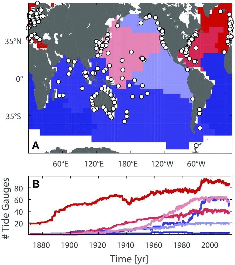
Spatial and temporal availability of tide gauges used in this study. (A) Spatial distribution of the tide gauges used in this study. Also shown are the six oceanic regions, which are used to build regional virtual stations. (B) Respective temporal availability of tide gauges for each region.

As a consequence, several reconstructions of GMSL changes have been published during the last decade, each of them based on different data subsets, methodological approaches, and tide gauge corrections. Among the most cited are refs. 1 and 2, which combined static spatial patterns constrained from satellite altimetry observations with temporal information from tide gauges into a global curve, showing a 20th century GMSL rise of 1.7 ± 0.3 mm⋅y⁻¹. Ref. 5 averaged regional sea level curves obtained from stacking rates of individual station data into a global reconstruction, leading to an increase of 1.9 ± 0.3 mm⋅y⁻¹ since 1900. These values, as well as others reported following similar approaches (3, 4), are consistent within their uncertainties and were subsequently adopted by the Fifth Assessment Report of the Intergovernmental Panel on Climate Change (9). More recently, ref. 6 developed a probabilistic approach that used tide gauges in combination with ensembles of model estimates for the spatial fingerprints of ocean dynamics, GIA, and ice melting, as well as an additional residual parameter for other local contributions to vertical land motion (VLM; such as tectonics or geomorphology), resulting in a significantly lower rate of 1.3 mm⋅y⁻¹. A set of sensitivity experiments indicated that their methodological approach was the primary reason for their estimate of a slower GMSL rate. Ref. 6 therefore suggested that previous studies have overestimated 20th century GMSL rise, and thus provided one possible solution of the enigma formulated more than a decade ago by Walter Munk (10).

This enigma points out that previous estimates of 20th century GMSL rise (e.g., refs. 1–5) are too linear and larger than estimates of the sum of individual contributions (thermal expansion, ice melt, and terrestrial water storage) (9). Although some attempts have been made to explain these discrepancies on the basis of underestimated sources (e.g., ref. 11), ref. 6 highlighted that their lower rate naturally balances the global sea level budget as the sum of modeled thermal expansion, glacier melting, and land water storage from the tabulations in the Fifth Assessment Report (9), without requiring any additional contribution from the ice sheets in Greenland and Antarctica. Ref. 12 recently extended this modeled GMSL budget with estimates of the contribution of the ice sheets, using Coupled Model Intercomparison Project Phase 5 (CMIP5) historical runs as forcing. However, as discussed in ref. 13, the GMSL reconstructions, especially those that show a larger 20th century trend, still exhibit remarkable differences from the CMIP5-based GMSL estimates. Particularly striking is a significant mismatch of observed and modeled GMSL between the 1930s and the 1970s, in which the models generally suggest lower rates than observations. Up to now, it is unclear whether this mismatch stems from poor model performances or uncertainties in individual GMSL reconstructions (both in variability and long-term trends) (13).

Although ref. 6 used probabilistic sea level fields to show why previous GMSL reconstruction approaches overestimated the rise before 1990, their tests have two general limitations: First, their values only account for a fraction of the GMSL overestimates during this period, and second, their sensitivity experiments rely on their reconstructed sea level field, rather than original tide gauges. Ref. 14 also suggested that the specific tide gauge selection of the ref. 6 study could have biased the 20th century GMSL toward lower rates. Specifically, they pointed toward the high uncertainties of Artic tide gauges, which were excluded in previous studies either because of the lack of altimetry data in the region or as a result of their questionable quality. In a very recent study, ref. 15 further investigated in Monte Carlo experiments the probability that 15 of the longest tide gauges (showing an average rate of 1.6 mm⋅y⁻¹) can be biased high or low, relative to the global mean, because of the contributions of ocean dynamics, GIA, and present-day ice melt. Assuming independence between the different sources, they suggested a probability of less than 1% that the rates obtained from these 15 tide gauge records are consistent with global mean rates lower than 1.4 mm⋅y⁻¹. These contrary arguments suggest that the spread between individual reconstructions is still poorly understood. Furthermore, none of the available reconstructions use local constraints on VLM, and they do not incorporate terrestrial freshwater storage (TWS) changes.

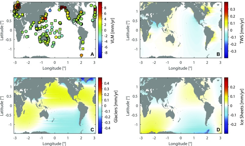
Here we present a GMSL reconstruction that accounts for ocean volume redistribution, local observations [mostly global positioning system (GPS)] of VLM, and geoid changes caused by ongoing GIA, present-day ice melt, and TWS, including groundwater depletion and water impoundment behind dams. We base our approach on an area-weighting average technique and on recent scientific achievements made for each individual correction. Our tide gauge selection is based on the data set described in ref. 16, consisting of 322 stations (Fig. S1A), for which VLM corrections with uncertainties of less than 0.7 mm⋅y⁻¹ are available (Materials and Methods and Fig. S2A). After accounting for VLM, each tide gauge is further corrected for geoid changes from ongoing GIA (17), glacier/ice-sheet melting (18–20) (Fig. S2 C and D), and TWS (21, 22) (Fig. S2B). The tide gauges are then grouped into six coherent regions objectively defined to account for water volume redistribution (Fig. S1A) (20). Ref. 23 demonstrated that these regions covary to some extent, so that an average between them cancels out some of the regional variability, leading to an improved estimate of the “true” GMSL. Within each oceanic region, a regional mean sea level curve is built by recursively combining the two nearest stations into a virtual station halfway, until only one station is left. The procedure is similar to the so-called virtual station technique developed by ref. 5, but with two important differences: first, to account for an unknown reference datum, we stack records adjusted for a common mean (i.e., removing in each record the mean of a common period of at least 19 y), rather than averaging their rates. Second, our GMSL reconstruction accounts for the spatial area of each of the six oceanic regions for which the virtual stations are representative. We use this straightforward approach because of its reproducibility, the ability to perform numerous sensitivity studies with limited computational effort, and the fact that ref. 23 obtained comparable results for the multidecadal variability in GMSL as more complex approaches based on empirical orthogonal functions (1).

Fig. S2.

Solid Earth and geoid corrections used in this study. (A) VLM [circles, GPS; square, altimetry minus tide gauge (AL-TG); diamonds, GIA] and geoid corrections resulting from (B) TWS, (C) glaciers, and (D) ice sheets.

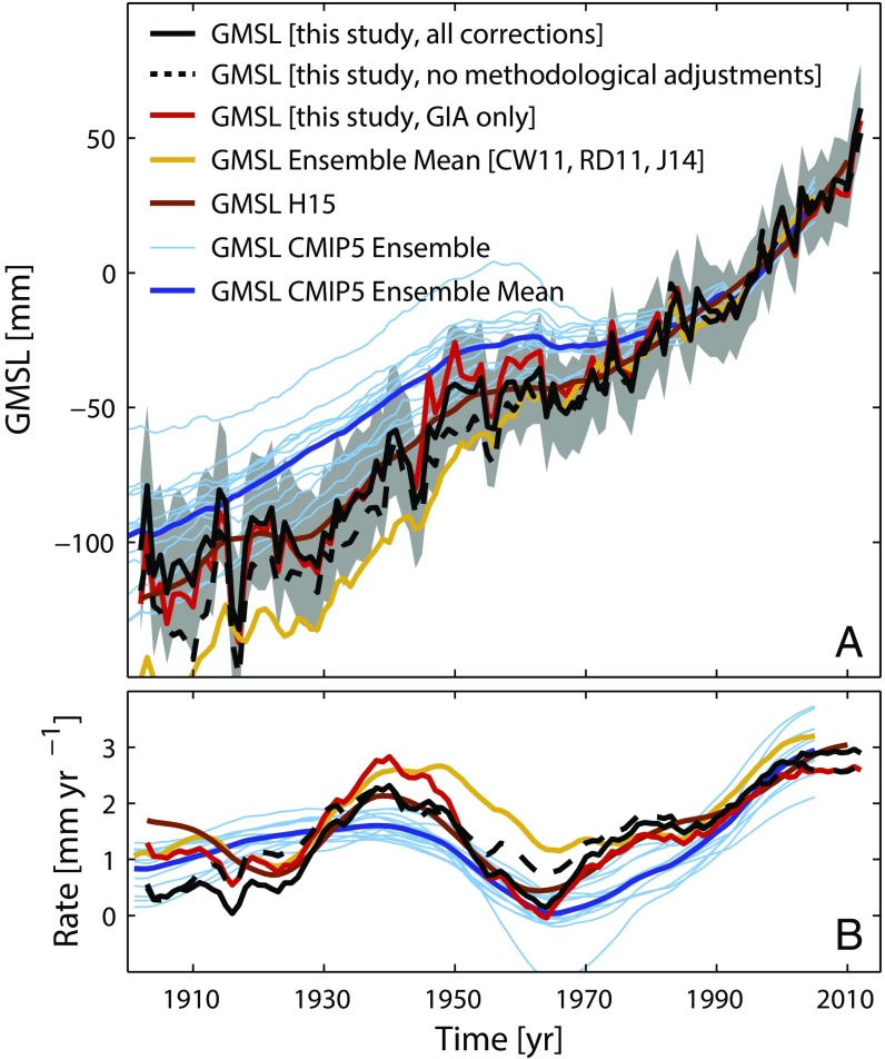
Our resulting GMSL reconstruction (using the subset for which the VLM uncertainty is smaller than 0.7 mm⋅y⁻¹) is displayed in Fig. 1A, indicating a long-term trend of 1.3 ± 0.2 mm⋅y⁻¹ (P > 0.99) since 1902 (here we report the error considering long-term persistent variability, as modeled in ref. 24). This value is consistent with ref. 6, but lower than those considered by the Fifth Assessment Report of the Intergovernmental Panel on Climate Change (9), represented here by the ensemble average of observed GMSL curves from refs. 1, 2, and 5 (rates of individual reconstruction can also be found in Fig. S3). During the period 1993–2012, our reconstruction yields a trend of 3.1 ± 1.4 mm⋅y⁻¹ (P ≥ 0.97), similar to the values obtained from independent satellite altimetry measurements (e.g., ref. 9). When comparing rates (Fig. 1B), there is a close correspondence of all tide gauge reconstructions after 1970, whereas before that time, some remarkable differences appear. For instance, our GMSL curve shows, as in ref. 6, rates close to zero at the beginning of the 1960s, whereby the manifestation of this drop is stronger than in earlier assessments (1, 2, 5), which yield minimum rates of only roughly 1 mm⋅y⁻¹. Before the 1960s, the reconstructions from refs. 1, 2, and 5 also suggest consistently larger rates than our GMSL curve, which is mainly related to our application of VLM and geoid corrections, rather than GIA only (Fig. 1B). These corrections play an increasingly important role in the earlier decades, in which the geographic bias of sparse tide gauge records is particularly strong (Fig. S1B) and might also explain the lower rates before ∼1920 compared with in ref. 6, which treated the VLM problem by using probabilistic model ensembles instead of local VLM observations, as used here. This also means that during this period, the robustness of our GMSL curve depends on the quality of the VLM and geoid corrections at a very few locations.

Fig. 1.

Time series and rates of GMSL during the period 1902–2012. (A) Revised GMSL reconstruction based on 322 tide gauges in comparison with previous estimates (CW11 = ref. 1; RD11 = ref. 2; J14 = ref. 5; H15 = ref. 6) and modeling attempts based on historical CMIP5 models (12). The gray shading marks the 1σ errors of the final reconstruction. The dotted black line represents a GMSL reconstruction with all VLM and geoid corrections, but without methodological adjustments such as area weighting and the use of a common mean. (B) The corresponding rates calculated with a singular spectrum analysis using an embedding dimension of 15 y.

Fig. S3.

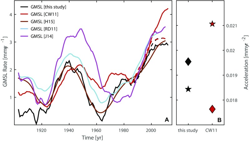
Comparison of GMSL rates from tide gauges and satellite altimetry. (A) Shown are the GMSL rates from ref. 1 (red) and our reconstruction (black), once based solely on tide gauges (solid lines), and once adjusted for GMSL from satellite altimetry (AVISO) since 1993 (dotted line). For comparison, the rates from ref. 2 (cyan), ref. 5 (magenta), and ref. 6 (brown) also are shown. (B) The corresponding acceleration coefficients (diamonds, adjusted; pentagrams, original). The figure demonstrates that the ref. 1 reconstruction overestimates GMSL since 1993 by up to 1 mm⋅y⁻¹, leading to a very large acceleration over the entire century. However, once adjusted for the “true” GMSL from AVISO satellite altimetry since 1993, the adjusted reconstructions closely follow our original reconstruction, leading to an overall acceleration that is smaller than that estimated for our original GMSL reconstruction.

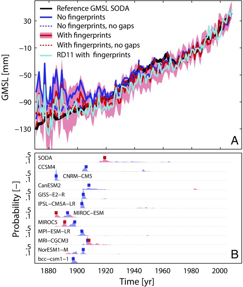
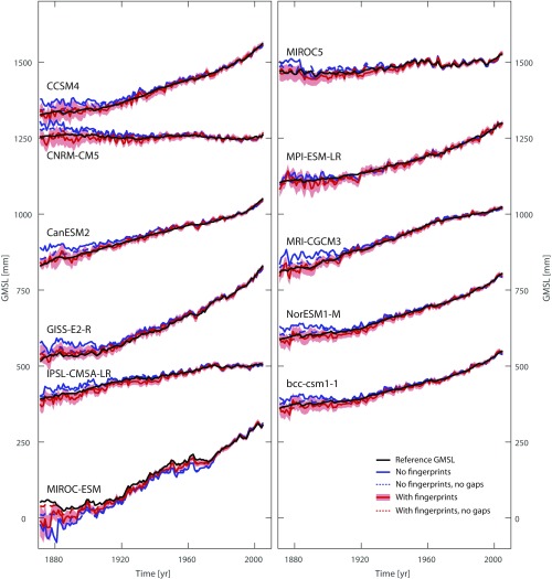
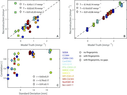
To explore whether the lower rates in our GMSL reconstruction (Fig. 1B) before ∼1970 are the result of methodological limitations with respect to the heterogeneous spatial and temporal tide gauge distribution, we test our approach in a set of 12 synthetic sea level fields from the Simple Ocean Data Assimilation (SODA) reanalysis and historical simulations of CMIP5 models during their common period from 1871 to 2005; these are combined with the corresponding components of the glacier contribution (in the case of SODA, the glacier reconstruction from ref. 18) and historical fingerprints from TWS (21, 22) and the Antarctic and Greenland ice sheets (19, 20) (Materials and Methods). Because in the synthetic sea level fields the true model GMSL, as well as the individual ice-melt and TWS fingerprints, are a priori known, they are an excellent testbed for our reconstruction approach. From each synthetic sea level field, we therefore assembled four different surrogate data sets, which are sampled at the 322 tide gauge locations used in reality (Materials and Methods), both with and without realistic data gaps and with and without corrections for the regional deviations from the global mean as a result of ice melt and TWS fingerprints. The comparison of the reconstructed GMSL curves with the true reference GMSL of each model (Fig. 2A for the SODA model and Fig. S4 for the 11 CMIP5 models) confirms it is indeed the availability of tide gauge records that primarily hampers robust GMSL estimates, leading to large biases mainly in the earlier decades around the turn of the century. To objectively identify the timing of these biases, we apply a Bayesian change point analysis (25) to the residuals between the reference GMSL and each tide gauge reconstruction. This analysis identifies the posterior probability of a statistically significant change in the residuals (P ≥ 0.95); that is, the timing at which our approach is no longer able to reconstruct the true model GMSL. We identify significant change points between 1885 and 1919 for all models without the consideration of local fingerprint corrections, but these change points disappear in eight models after correcting individual tide gauge surrogates for their respective TWS and ice melt fingerprints (Fig. 2B). From the remaining four models, only two, SODA and MRI-CGCM3, suggest significant change points after 1902 (1919 and 1908, respectively), whereby their influence on the long-term trends since 1902 is only minor in the respective models (0.04 and 0.03 mm⋅y⁻¹, respectively (Fig. S5B). In general, the application of spatially varying corrections associated with ice melt and TWS fingerprints reduces the trend biases in models from −0.45 ± 1.17 mm⋅y⁻¹ (median ± standard deviation of the entire ensemble) to −0.02 ± 0.70 mm⋅y⁻¹ before 1902 (Fig. S5A). Although some uncertainties in the GMSL reconstructions still persist, most models indicate a reasonable performance (trend differences, 0.10 ± 0.07 mm⋅y⁻¹ with fingerprint corrections compared with 0.14 ± 0.14 mm⋅y⁻¹ without fingerprint corrections) of our approach with respect to long-term changes during the entire 20th century (Fig. S5B).

Fig. 2.

Performance of the area-weighted average approach in ocean models. (A) Sensitivity of the area-weighted average technique in the SODA reanalysis (its reference GMSL is shown by the black line) to the four initial data sets: Gaps as in reality, no fingerprint corrections applied (dark blue); assuming a full record, no fingerprint corrections applied (dark blue dotted); gaps as in reality, fingerprint corrections applied (red, with shading noting its 1σ uncertainty); and assuming a full record, fingerprint corrections applied (red dotted) (Fig. S3 for the respective curves from the 11 CMIP5-based synthetic sea level fields). The cyan curve represents a GMSL reconstruction with gaps as in reality and fingerprint corrections applied, but using the tide gauge subset from ref. 2. (B) Results of the Bayesian change point analysis (25) on the differences between each model specific reference GMSL and corresponding tide gauge reconstruction , without fingerprint corrections; red, with fingerprint correction) in each model. The change point analysis provides statistically the probability and timing of changes (shaded areas) in the relationship between the “true” model GMSL and its reconstruction. Tall, thin spikes suggest relative certainty in the timing of a change point, whereas wider spikes suggest more uncertainty in its timing. The red and blue squares mark the most probable timing from 500 iterations.

Fig. S4.

Performance of the area-weighted average technique in synthetic sea level fields from the CMIP5 database. Comparison of reconstructed GMSL with the “true” reference GMSL in the 11 synthetic sea level fields based on CMIP5 historical simulations (dynamic sea level and glaciers) and reanalysis estimates of TWS and ice sheet melting. The sensitivity is tested for different initial data sets, as defined in the caption of Fig. 2 (showing the results for the GMSL from the SODA reanalysis).

Fig. S5.

Trend and correlation biases in GMSL reconstructions based on synthetic sea level fields from ocean models. (A) Comparison between the linear trends for the reference GMSL of each model and its reconstruction based on tide gauges with (squares) and without (circles) fingerprint corrections and assuming no gaps in tide gauge records (i.e., a fully available record; diamonds) for the period 1871–1902. (B) As A, but for the period 1902–2005. (C) Relationship between the correlation of the reference GMSL and its tide gauge reconstruction in each model and the respective interannual variability of the reference GMSL (SD). The results suggest that the GMSL can be better reconstructed in models with stronger interannual variability.

We also tested whether our approach is able to reconstruct the interannual to multidecadal GMSL variability in the synthetic model fields (Fig. S5C). We find that our approach sufficiently reproduces the variability patterns in most models if all fingerprint corrections are applied (r = 0.78 ± 0.17 and r = 0.63 ± 0.21 with and without fingerprint corrections, respectively), whereby again, a strong coupling to the availability of tide gauge records is recognized (r = 0.91 ± 0.11, assuming full tide gauge records without any gaps) (Fig. S5C). In SODA (the only model that assimilates temperature and salinity observations), a large drop after the volcanic eruption of Mount Agung from 1963 (e.g., ref. 11) is not well reproduced because of incomplete tide gauge records (Fig. 2A), leading to a poorer representation of the interannual variability (r = 0.45) compared with the CMIP5-based models (r = 0.79 ± 0.15) (Fig. S5C). However, reconstructions of GMSL from other CMIP5 models showing comparably large drops at the same time [e.g., NASA Goddard Institute for Space Studies (GISS)-E2-R, Model for Interdisciplinary Research on Climate (MIROC)-ESM] perform well in reproducing such variations (r = 0.95 and r = 0.79, respectively) (Figs. S4 and S5C). Furthermore, in reality, our GMSL curve shows, together with that of ref. 6, the most pronounced drop of all reconstructions (Fig. 1B). This (together with the lower rates before) leads also to a better agreement with the historical CMIP5 simulations of the GMSL budget compiled by ref. 12, which indicate generally more moderate rates between the 1930s and 1970s than the tide gauge reconstructions from refs. 1, 2, and 5 (Fig. 1B).

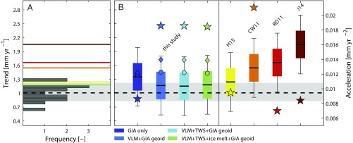
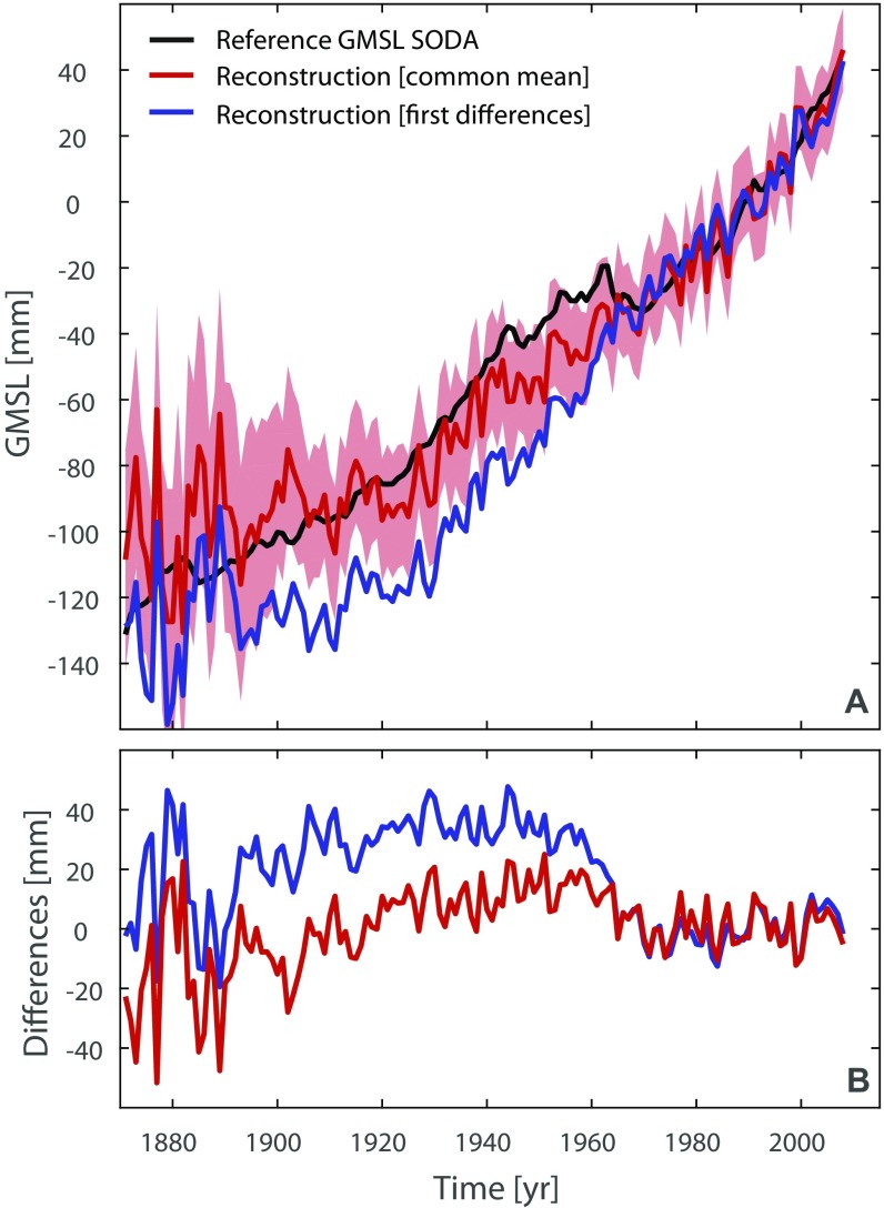
To further examine the influence of methodological adjustments as well as VLM and geoid corrections on prealtimetry GMSL rates, we produced a set of observation-based reconstructions with and without individual adjustments and corrections and calculated linear trends from 1902 to 1990 (Fig. 3B). First, we consecutively introduced the VLM and the individual geoid corrections for TWS and ice melt in each tide gauge record. The corrections significantly reduce the spatial variability in each subregion with a particularly striking reduction in the Northeast Pacific (Fig. S6). In particular, the tide gauges along the coast of Alaska are strongly affected by the corrections. In most cases, the corrections lead to a reduction in the overall rate for the entire region, and therefore also in the resulting GMSL, accounting for ∼0.2–0.3 mm⋅y⁻¹ of the obtained differences compared with earlier estimates, whereby VLM itself plays the most important role (Fig. 3B). This contrasts with recent results by ref. 26, finding a VLM influence on GMSL of the opposite sign, but considering only large-scale VLM effects rather than local movements at the individual tide gauges. Second, we test the influence of using a common mean, rather than stacking first differences, which was the preferred approach in most previous studies (e.g., refs. 1, 4, and 5) for solving the problem of an uncommon reference datum between individual tide gauges (colored diamonds in Fig. 3B). Using a common mean also results in ∼0.2–0.3 mm⋅y⁻¹ lower trends than stacking rates. This is because of drifts resulting from an error accumulation in the integration process of the virtual stations that is especially relevant for the lower frequencies (2) (Fig. S6) and leads to artificially large rates in GMSL before ∼1960 (see sensitivity experiment in the SODA fields in Fig. S7). Comparing the corresponding six regional curves with the individual tide gauge records in each oceanic region suggests everywhere larger correlations when a common mean adjustment is used (Fig. S6). Third, we reconstructed the GMSL with and without area weighting (colored dots in Fig. 3B). Regional averaging to reconstruct GMSL with and without area weighting leads to differences of 0.2–0.3 mm⋅y⁻¹ because of the larger influence of comparably small areas (lowest trends before 1990 have been found in the Indian Ocean and South Pacific region, the South Atlantic, and the Northwest Pacific; Fig. S8). The combination of all adjustments and corrections sums to ∼0.6–0.9 mm⋅y⁻¹, which potentially explains all the differences compared with earlier assessments (refs. 1–5) of the 1902–1990 period. For the same period, the sum of modeled contributions from the 14-member CMIP5 model ensemble by ref. 12 (SI Text) shows a median trend of 1 mm⋅y⁻¹ (1σ bounds of 0.83–1.22 mm⋅y⁻¹) (Fig. 3A), which is consistent with our final GMSL estimate of 1.1 ± 0.3 mm⋅y⁻¹ (P > 0.99) containing all necessary corrections (Fig. 3 A and B). However, with the exception of ref. 6, all other published reconstructions clearly fall outside the range of modeled contributions (Fig. 3A).

Fig. 3.

Linear trends in observed and modeled GMSL during the period 1902–1990. (A) Linear trend frequency in the CMIP5 GMSL ensemble from ref. 12 (dark gray bars), together with the median value (thick dotted line) and the 68% confidence bounds (light gray shading). The color coding follows B. (B) Linear trends of four different GMSL realizations based on different corrections applied in comparison with previous estimates with their respective uncertainties (based on ref. 25) as boxplots (1σ and 2σ uncertainties). The dots correspond to the trends when no area weighting is applied, whereas the diamonds provide trend estimates for the reconstructions based on rate stacking without area-weighting as in ref. 5. Also shown is the acceleration term (pentagrams, right y axis) for each reconstruction extracted from the first differences of the nonlinear trends during the entirely available period of each reconstruction since 1902.

Fig. S6.

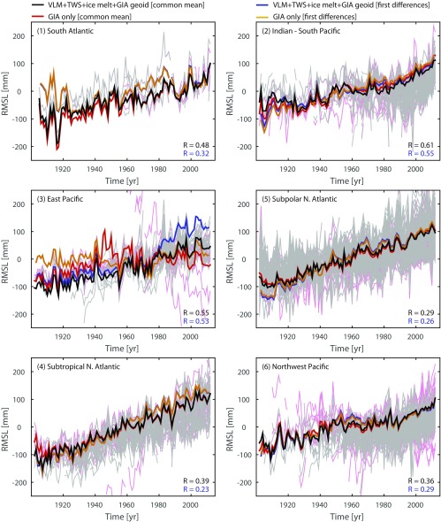
Virtual stations for the six oceanic regions based on different stacking approaches and corrections. Shown are the individual tide gauge records corrected for VLM, TWS, ice melting, and GIA geoid (gray) or just GIA (light red) and their respective virtual stations based on two different stacking approaches: averaging after removing a common mean, and stacking first differences (also known as rate stacking; see legend for a description of the line colors). Both approaches are used to overcome the problem of an unknown reference datum of individual tide gauges. Also provided for each region are the medians of linear correlations between the virtual stations and individual tide gauge records from both approaches (black and blue R values).

Fig. S7.

Comparison of the reference GMSL in SODA to two different reconstructions. (A) Reference GMSL (black line) and reconstructions using either a common mean between individual tide gauges (red line, shaded area gives the 1σ uncertainty) or first differences (blue curve). (B) Differences between the reference GMSL and the two reconstructions.

Fig. S8.

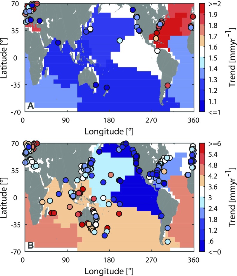
Trends in individual tide gauges corrected for VLM and geoid changes from TWS and ice melt. (A) Trends in tide gauges providing at least 70 y of data during the period 1902–2012. Blue colors denote trends equal or smaller than 1.5 mm⋅y⁻¹, and white and red dots mark those stations providing long-term trends above 1.5 mm⋅y⁻¹. The colored shaded areas represent the trends of the region-specific virtual stations. (B) Trends in tide gauge records providing at least 15 y of data during the period 1993–2012. Blue colors denote trends equal or smaller than 3 mm⋅y⁻¹, whereas white and red dots mark those stations providing long-term trends above 3 mm⋅y⁻¹.

The downward correction of previous presatellite altimetry GMSL estimates in combination with the close correspondence between satellite altimetry, historic CMIP5 simulations, and our GMSL reconstruction after 1993 (Fig. 1B) has another important consequence: the trend difference between both periods leads to an acceleration (here estimated with a linear fit to the first differences of the nonlinear trend obtained with a singular spectrum analysis, using a smoothing window equal to 15 y and uncertainties obtained with a bootstrapping approach producing 100 surrogates) of 0.018 ± 0.008 mm⋅y⁻² (P > 0.99) in GMSL, which is almost twice as large as in all other reconstructions (including ref. 6) except the ref. 1 estimate (Fig. 3B). However, the rates of the GMSL reconstruction by ref. 1 are, with values exceeding 4 mm⋅y⁻¹, biased high compared with satellite altimetry since 1993 (Fig. S3A). To test the influence of this overestimation during the satellite altimetry period, we have substituted the satellite-based GMSL reconstruction from Archiving, Validation and Interpretation of Satellite Oceanographic data (AVISO) into ours, and the reconstruction of ref. 1 for the period 1993–2012 (Fig. S3A). Although our estimate is only barely affected by the adjustment (rates and acceleration become slightly higher), the acceleration in the ref. 1 reconstruction decreases considerably, leading to a smaller value than in our reconstruction (Fig. S3B). This shows that the larger acceleration in the ref. 1 reconstruction should be considered with care. The acceleration in our GMSL curve is mainly determined by a transition from slower-than-average rates before 1990 (Fig. S8A) toward unprecedented high rates during the last 2 decades in the Indian Ocean South Pacific sector (Fig. S8B), which is consistent with an asymmetry in ocean mass redistribution between the Northern and Southern Hemisphere, as suggested in ref. 23. The acceleration in GMSL is, further, consistent with recent findings that the anthropogenic contribution to GMSL (dominated by glacier melting and thermosteric sea level rise) has increased during the 20th century, from less than 16% before 1950 to more than 69% after 1970 (12, 27, 28).

We have reassessed 20th century GMSL estimates from tide gauges by combining recent advances in solid Earth and geoid corrections related to VLM, TWS, and glacier/ice sheet melting with an improved technique canceling out ocean mass redistribution between individual regions (23). Our technique is simple and computationally efficient and allows us to evaluate the influence of each applied correction on GMSL estimates. The resulting GMSL curve shows, in agreement with ref. 6, significantly smaller trends compared with former and widely accepted GMSL estimates (9).This smaller rate is geographically dominated by slower-than-average sea level rise in the less well-instrumented Southern Hemisphere (29) and the Northwest Pacific compared with slightly larger-than-average rates in the North Atlantic (Fig. S8). The resulting trend gradient between the different regions is broadly consistent with the possible sea level imprint of a 20th century slowdown of the Atlantic Meridional Overturning Circulation (30), known from ocean model experiments (31), which, however, requires further investigations in future studies. Sensitivity experiments on the reasons for our lower prealtimetry GMSL rate compared with earlier attempts suggest roughly one-third of the obtained differences are related to biases stemming from regional variability caused by VLM, TWS, and ice melt, whereas two-thirds can be considered methodological; that is, resulting from an improved consideration of the geometry of regional sea level (here simple area-weighting) and a solution for overcoming the varying reference datum in individual tide gauge records (here a common mean). In contrast to ref. 15, which considered GMSL rates below 1.4 mm⋅y⁻¹ to be extremely unlikely, we used observational estimates of VLM and the spatial bias at tide gauges resulting from sea level fingerprints, thus avoiding any assumption about dependencies between different sea level contributions. Because our approach is different from that of ref. 6, our results provide an independent confirmation of their suggestion of a relatively slow prealtimetry rate of GMSL rise. Our constraint of 1.1 ± 0.3 mm⋅y⁻¹ (P > 0.99) during this period, in turn, explains the majority of the observed differences between individual reconstructions and recently modeled contributions to GMSL rise from the CMIP5 ensemble between the 1930s and 1970s, thus increasing our confidence in process-based models that are an indispensable tool for future projections (9).

SI Text

For comparing our GMSL curve with historical runs from CMIP5 models, we have used the sum of individually modeled contributions obtained by ref. 12. In this model data set, the output of the historical runs from CMIP5 climate models were used to derive GMSL contributions for the period 1900–2005. These contributions include: GMSL changes resulting from thermal expansion, corrected for drifts with the respective preindustrial control runs; glacier contributions obtained by forcing a global glacier evolution model with CMIP5 air temperatures and precipitation; and surface mass balance estimates from Greenland and Antarctica ice sheets. Contributions from TWS for the period 1900–2005 and from observed ice sheet dynamic processes (only for the period 1993–2005, as it is assumed to be negligible before) were also included. Further details on the computation can be found in ref. 12.

Materials and Methods

Area-Weighted Average Technique.

Tide gauges only poorly sample the global ocean, and their distribution has a large bias toward the Northern Hemisphere, especially in the earlier decades of the 20th century (Fig. S1). To overcome this bias, ref. 5 introduced a virtual station technique, in which the global ocean is divided into 12 coastal regions. For each coastal region, the two closest stations are recursively identified and stacked to a virtual station weighted by their distance (for details on the error calculation, see ref. 32). The 12 finally resulting virtual stations are then later further merged into a global curve. However, the final merging does not contain any further area weighting, as the representativeness of the virtual station for a certain open ocean region is not known. Here we adopt the general idea of the approach, but improve it in several ways. First, we use different oceanic regions, which are based on an objective cluster analysis by ref. 23. The authors identified six coherently varying oceanic regions (Fig. S1A) from satellite altimetry and showed that a certain number of tide gauges are able to describe the multidecadal variations within each region. The selection of these regions allows us to better sample the entire ocean and, more important, provides an estimate of the area for which each virtual station is representative. Hence, each virtual station can later be weighted before being merged into a global mean. The second adjustment is related to the reference problem of individual tide gauges. Because there is no common reference datum for the tide gauge records, ref. 5 stacked rates of mean sea level. However, one drawback of this approach is that small errors in individual estimates can inflate as the series is integrated backward, with the lowest frequencies being most susceptible to errors (2). As a result, the final global curve may drift away from the “truth,” especially in the earlier years, where the uncertainties are significantly higher than in recent decades. To overcome this problem, we stack two stations into a virtual station by simply adjusting both records to a common mean. This, of course, presumes that two records always share a common period, which is the case in our tide gauge selection. The error propagation from an individual tide gauge toward the global mean is calculated following the approach of ref. 5 and ref. 32, which uses the geographical location of individual tide gauges.

Tide Gauge Records and Corrections.

We use an initial data set of 448 tide gauge records from the Permanent Service of Mean Sea Level (7) for which VLM corrections from either GPS or tide gauge minus altimetry were available (15). The records are corrected for the mean seasonal cycle by fitting an annual and semiannual harmonic to the monthly raw data. Also removed is the inverse barometer effect caused by the hydrostatic response of the ocean to sea level pressure fluctuations around the spatial mean of the sea level pressure over the ocean (33), using the Twentieth-Century Reanalysis Project version 2 data set (34).

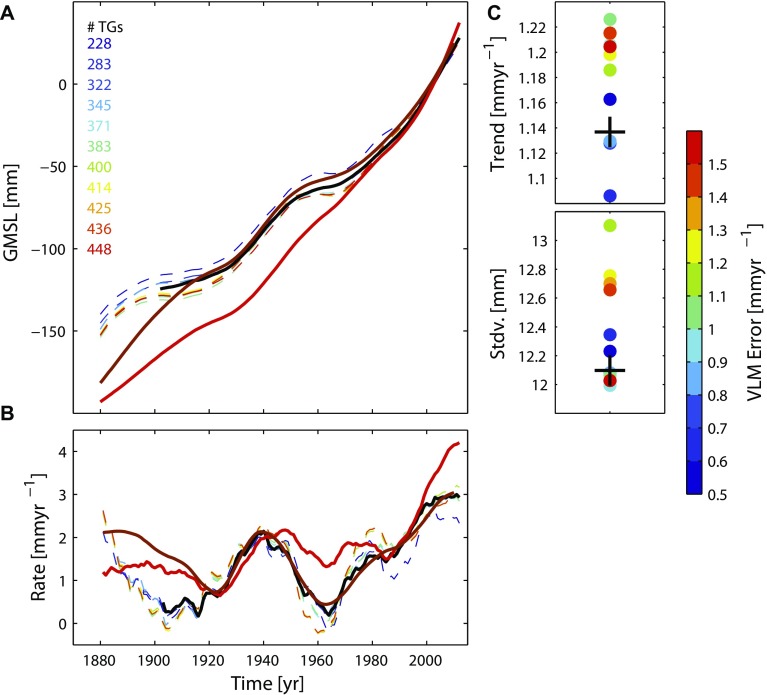
VLM at tide gauges is adopted from ref. 16 (Fig. S2A). Stations for which a continuous GPS station is available are adjusted using the rates and uncertainties provided by Universite de La Rochelle (ULR)6a (note that this is an update of ref. 16, which used ULR5). If GPS is not available at a particular station, VLM is alternatively determined by differencing altimetry and tide gauge time series for their common period. Uncertainties are computed considering the noise content in the differenced time series as a combination of white noise and power law noise of an a priori unknown spectral index (16). The accuracy of the VLM correction is used to derive 11 different subsets of tide gauges; namely, only those for which VLM is known with an uncertainty smaller than 0.5 mm⋅y⁻¹ (228 stations), 0.6 mm⋅y⁻¹ (283 stations), or 1.5 mm⋅y⁻¹ (448 stations). The subset with an uncertainty smaller than 0.7 mm⋅y⁻¹ (322 stations) is used for our final GMSL curve, which represents a trade-off between good data coverage and robust VLM estimates. Note that the differences between the GMSL curves from different tide gauge subsets based on VLM errors were found to be small (Fig. S9). Selection criteria based on earlier assessments (2) (e.g., only the longest tide gauges with high confidence on their quality) also showed only minor differences compared with our subsets in the SODA test fields (Fig. 2A), as well as observational data (1.3 mm⋅y⁻¹ compared with our final estimate of 1.1 mm⋅y⁻¹ before 1990), with VLM corrections applied only to those tide gauges that are covered in both subsets. For the comparison with earlier assessments, a GIA-only correction is applied. In this case, the ICE5G model by ref. 17 is used.

Fig. S9.

Effect of tide gauge selection on GMSL and extension to 1880. (A) Shown are 11 realizations of our GMSL curve, using different subsets of tide gauges resulting from VLM error thresholds between 0.5 and 1.5 mm⋅y⁻¹, extending back to 1880 (dashed lines). Since before 1902, there is no information on the geoid corrections; these curves are corrected only for VLM. The GMSL curve from Fig. 3A, including all corrections, is shown for comparison in black. Also shown are the reconstructions from refs. 1 and 6 (solid red and brown lines, respectively). (B) Corresponding rates. (C) Linear trends (1902–1990) and SDs (1902–2012) from each reconstruction (colored dots) shown in A and the final curve from Fig. 3A (black cross).

Changes in TWS (either caused by groundwater depletion or water impoundment behind dams) are accompanied by regional deflections of the solid earth (crustal motion) and sea surfaces (geoid), which can be calculated using Green’s functions for vertical displacement and gravitational potential (21, 22). For water impoundment behind dams, we use updated fields calculated by ref. 22 from 1902 to 2014, which are based on a combination of the global reservoir data sets from ref. 35 and ref. 36 (see ref. 22 for further details) consisting of 674 of the largest reservoirs. For groundwater depletion, we adopt the fields from ref. 21, updated for the entire period from 1902 to 2014 and scaled to match recent estimates (37). Specifically, we used spatial variations from the hydrological model of ref. 38, which expresses groundwater depletion in a yearly resolution on a 0.5° × 0.5° grid, and the scaled depletion rates everywhere by a factor of 0.8 so that total groundwater depletion matches the results of updated hydrological models (37). Because the crustal motion component is already approximated by the VLM correction, we only correct for spatial variations in the geoid response resulting from loading by changes in TWS (i.e., deflections about a zero mean).

The same applies to the regional fingerprints from ice melting. To account for the regional deflections after freshwater injections from glaciers and ice sheets into the ocean, we calculated fingerprints for updated sea level equivalents of 18 major glacier regions and ice sheet mass balance discharge estimates of the Greenland and Antarctic ice sheets. The glacier fingerprints are based on reconstructions from ref. 18 and their update in ref. 39. The Greenland ice sheet contribution to sea level is estimated using the recent mass balance estimate from ref. 19. The Antarctic ice sheet is modeled with the RACMO2.3 model (40), as in ref. 20, assuming no mass changes before 1979, long-term balance between the surface mass balance from RACMO2.3 and ice discharge between 1979 and 1993, and small acceleration in ice discharge after 1993 to match GRACE estimates (20). The fingerprints for the ice melt contributions are calculated by solving the elastic sea level equation, as described by ref. 41. The rotational feedback is included following ref. 42. As for TWS, we only considered the geoid response to the loading, which determines the regional deviations from the global mean.

Synthetic Sea Level Data.

One general problem of all tide gauge-based GMSL reconstructions is that there is no observational validation option over more than two decades (satellite altimetry) available. An alternative possibility to test our approach is the use of artificial ocean model fields, in which the “true” model GMSL is a priori known. However, so far there are no CMIP5 models available integrating simulations of the ocean and the cryosphere into coupled runs, so that except for the dynamic sea surface height, each individual component has to be calculated offline. To produce homogeneous synthetic fields of historical sea level fields, we combine historical fields of sea surface height from CMIP5 models and the SODA reanalysis over the period from 1871 to 2005 with independent estimates of glacier melting (18). Also added are the observation-based estimates of the ice sheets (19, 20) and TWS containing both groundwater depletion (21) and water impoundment behind dams (22). For the simulation of ocean dynamics, sea surface height fields (variable “zos” in CMIP5 terminology) are obtained from the historical simulations of 11 CMIP5 models (Fig. S3 for the models). For each model run, the globally averaged steric sea level (variable “zosga”), corrected (quadratic fit to the control runs) for drifts resulting from the short spin-up and integration time of the historical runs (11), is added to the sea surface height to account for global ocean volume changes within the model (43). CMIP5 runs were not further corrected for omitted preindustrial volcanic forcing or additional drifts (see also ref. 12), as these corrections are globally uniform and will therefore not affect our model internal tests of the GMSL reconstruction technique. The SODA reanalysis (44) is also used and processed in the same way. Sea level changes associated with glacier melting (i.e., their total GMSL contribution including the respective regional fingerprint) are added to the modeled sea surface heights by multiplying the CMIP5 model-specific glacier reconstruction from ref. 18 and ref. 39 with the respective fingerprint from ref. 45. For the SODA model, the observational glacier reconstruction based on Hadley Centre and the Climate Research Unit (HADCRU) forcing is used (18). All model fields are supplemented with the same observational fields of the ice sheet and TWS contribution to sea level. For each modeled sea level field, a GMSL was reconstructed on the basis of the area-weighted average technique applied to the grid point time series next to the real-world locations of tide gauges and then compared with the “true” reference GMSL of each model.

Trend Uncertainties in Individual GMSL Reconstructions.

The calculation of linear trends is susceptible to a series of high/low values at the end of the time series. The corresponding uncertainty is usually addressed by simulating the natural variability, represented by the residuals around the trend line, in Monte-Carlo experiments under the assumption that it follows a specific noise process (e.g., ref. 46). Although it has been widely accepted that an autoregressive process of the order 1 is suitable for this purpose (e.g., ref. 9), recent studies demonstrate that the use of long-memory processes provides a physically more consistent description of the noise (24, 28, 47–50). Ref. 24 further pointed out that none of the available GMSL reconstructions provides a proper description of the natural GMSL variability, as they are “trained” to reproduce the long-term trends (4). The authors therefore provided an improved estimate on the basis of ocean reanalysis data, which is used here uniformly for each GMSL reconstruction.

References

- 1.Church JA, White NJ. Sea-level rise from the late 19th to the early 21st Century. Surv Geophys. 2011;32:585–602. [Google Scholar]
- 2.Ray RD, Douglas BC. Experiments in reconstructing twentieth-century sea levels. Prog Oceanogr. 2011;91:496–515. [Google Scholar]
- 3.Wenzel M, Schroeter J. Reconstruction of regional mean sea level anomalies from tide gauges using neural networks. J Geophys Res. 2010;115:C08013. [Google Scholar]
- 4.Calafat FM, Chambers DP, Tsimplis MN. On the ability of global sea level reconstructions to determine trends and variability. J Geophys Res. 2014;119:1572–1592. [Google Scholar]
- 5.Jevrejeva S, Moore JC, Grinsted A, Matthews AP, Spada G. Trends and acceleration in global and regional sea levels since 1807. Global Planet Change. 2014;113:11–22. [Google Scholar]
- 6.Hay CC, Morrow E, Kopp RE, Mitrovica JX. Probabilistic reanalysis of twentieth-century sea-level rise. Nature. 2015;517:481–484. doi: 10.1038/nature14093. [DOI] [PubMed] [Google Scholar]
- 7.Holgate SJ, et al. New data systems and products at the Permanent Service for Mean Sea Level. J Coast Res. 2013;29:493–504. [Google Scholar]
- 8.Kopp RE, Hay CC, Little CM, Mitrovica JX. 2015. Geographic variability of sea-level change. Curr Clim Change Rep 2015;1:192.
- 9.Church JA, et al. 2013. Sea Level Change. Climate Change 2013: The Physical Science Basis. Contribution of Working Group I to the Fifth Assessment Report of the Intergovernmental Panel on Climate Change, Chapter 13, eds Stocker TF, et al. (Cambridge Univ. Press)
- 10.Munk W. Twentieth century sea level: An enigma. Proc Natl Acad Sci USA. 2002;99:6550–6555. doi: 10.1073/pnas.092704599. [DOI] [PMC free article] [PubMed] [Google Scholar]
- 11.Gregory J, et al. Global mean-sea level rise: Is the whole greater than the sum of all prats? J Clim. 2013;26:4476–4499. [Google Scholar]
- 12.Slangen ABA, et al. 2016. Anthropogenic forcing dominates global mean sea-level rise since 1970. Nat Clim Chang 2016;6:701–705.
- 13.Dangendorf S. 2016. Human influence on sea-level rise. Nature Climate Change 2016;6:661–662.
- 14.Hamlington BD, Thompson PR. Considerations for estimating the 20th century trend in global mean sea level. Geophys Res Lett. 2015;42:4102–4109. [Google Scholar]
- 15.Thompson PR, et al. Are long tide gauge records in the wrong place to measure global mean sea level rise? Geophys Res Lett. 2016;43:403–410. [Google Scholar]
- 16.Wöppelmann G, Marcos M. Vertical land motion as a key to understanding sea level change and variability. Rev Geophys. 2016;54:64–92. [Google Scholar]
- 17.Peltier WR. Global glacial isostacy and the surface of the Ice-Age Earth: The ICE5G(VM2) model and GRACE. Annu Rev Earth Planet Sci. 2004;32:111–149. [Google Scholar]
- 18.Marzeion B, Jarosch AH, Hofer M. Past and future sea-level change from the surface mass balance of glaciers. Cryosphere. 2012;6:1295–1322. [Google Scholar]
- 19.Kjeldsen KK, et al. Spatial and temporal distribution of mass loss from the Greenland Ice Sheet since AD 1900. Nature. 2015;528:396–400. doi: 10.1038/nature16183. [DOI] [PubMed] [Google Scholar]
- 20.Frederikse T, et al. Closing the sea level budget on a regional scale: Trends and variability on the Northwestern European continental shelf. Geophys Res Lett. 2016;43:10864–10872. doi: 10.1002/2016GL070750. [DOI] [PMC free article] [PubMed] [Google Scholar]
- 21.Veit E, Conrad CP. The impact of groundwater depletion on spatial variations in sea level change during the past century. Geophys Res Lett. 2016;43:3351–3359. [Google Scholar]
- 22.Fiedler JW, Conrad CP. Spatial variability of sea level rise due to water impoundment behind dams. Geophys Res Lett. 2010;37:L12603. [Google Scholar]
- 23.Thompson PR, Merrifield MA. A unique asymmetry in the pattern of recent sea level change. Geophys Res Lett. 2014;41:7675–7683. [Google Scholar]
- 24.Dangendorf S, et al. Detecting anthropogenic footprints in sea level rise. Nat Commun. 2015;6:7849. doi: 10.1038/ncomms8849. [DOI] [PMC free article] [PubMed] [Google Scholar]
- 25.Ruggieri E. A Bayesian approach to detecting change points in climatic records. Int J Climatol. 2013;33:520–528. [Google Scholar]
- 26.Hamlington BD, et al. Assessing the impact of vertical land motion on twentieth century global mean sea level estimates. J Geophys Res. 2016;121:4980–4993. [Google Scholar]
- 27.Kopp RE, et al. Temperature-driven global sea-level variability in the Common Era. Proc Natl Acad Sci USA. 2016;113:E1434–E1441. doi: 10.1073/pnas.1517056113. [DOI] [PMC free article] [PubMed] [Google Scholar]
- 28.Marcos M, et al. 2016. Internal variability versus anthropogenic forcing on sea level and its components. Surv Geophys 2017;38:329.
- 29.Wöppelmann G, et al. Evidence for a differential sea level rise between hemispheres over the twentieth century. Geophys Res Lett. 2014;41:1639–1643. [Google Scholar]
- 30.Rahmstorf S, et al. Exceptional twentieth-century slowdown in Atlantic Ocean overturning circulation. Nat Clim Chang. 2015;5:475–480. [Google Scholar]
- 31.Levermann A, et al. Dynamic sea level changes following changes in the thermohaline circulation. Clim Dyn. 2005;24:347–354. [Google Scholar]
- 32.Jevrejeva S, Grinsted A, Moore JC, Holgate S. Nonlinear trends and multiyear cycles in sea level records. J Geophys Res. 2006;111:C09012. [Google Scholar]
- 33.Ponte RM. Low-frequency sea level variability and the inverted barometer effect. J Clim. 2006;23:619–629. [Google Scholar]
- 34.Compo GP, et al. The twentieth century reanalysis project. Q J R Meteorol Soc. 2011;137:1–28. [Google Scholar]
- 35.Vorosmarty CJ, et al. The storage and aging of continental runoff in large reservoir systems of the world. Ambio. 1997;26:210–219. [Google Scholar]
- 36.Chao BF, Wu YH, Li YS. Impact of artificial reservoir water impoundment on global sea level. Science. 2008;320:212–214. doi: 10.1126/science.1154580. [DOI] [PubMed] [Google Scholar]
- 37.Wada Y, et al. Fate of water pumped from underground and contributions to sea-level rise. Nat Clim Chang. 2016;6:777–780. [Google Scholar]
- 38.Wada Y, et al. Past and future contribution of global groundwater depletion to sea-level rise. Geophys Res Lett. 2012;39:L09402. [Google Scholar]
- 39.Marzeion B, Leclercq PW, Cogley JG, Jarosch AH. Brief Communication: Global reconstruction of glacier mass change during the 20th century are consistent. Cryosphere. 2015;9:2399–2404. [Google Scholar]
- 40.Noel B, et al. Evaluation of the updated regional climate model RACMO2.3: Summer snowfall impact on the Greenland ice sheet. Cryosphere. 2015;9:1831–1844. [Google Scholar]
- 41.Mitrovica JX, Wahr J, Matsuyama I, Paulson A. The rotational stability of an ice-age earth. Geophys J Int. 2005;161:491–506. [Google Scholar]
- 42.Tamisiea ME, et al. Impact of self-attraction and loading on the annual cycle in sea level. J Geophys Res. 2010;115:C07004. doi: 10.1029/2009JC005687. [DOI] [Google Scholar]
- 43.Griffies SM, Greatbatch RJ. Physical processes that impact the evolution of global mean sea level in ocean climate models. Ocean Model. 2012;51:37–72. [Google Scholar]
- 44.Carton FM, Giese BS. A reanalysis of ocean climate using Simple Ocean Data Assimilation (SODA) Mon Weather Rev. 2008;136:2999–3017. [Google Scholar]
- 45.Bamber J, Riva REM. The sea level fingerprint of recent ice mass fluxes. Cryosphere. 2010;4:621–627. [Google Scholar]
- 46.Visser H, Dangendorf S, Peterson A. A review of trend models applied to sea level data with reference to the “acceleration-deceleration debate”. J Geophys Res. 2015;120:3873–3895. [Google Scholar]
- 47.Bos MS, Williams SDP, Araujo IB, Bastos L. The effect of temporal correlated noise on the sea level rate and acceleration uncertainty. Geophys J Int. 2014;196:1423–1430. [Google Scholar]
- 48.Dangendorf S, et al. Evidence for long-term memory in sea-level. Geophys Res Lett. 2014;41:5564–5571. [Google Scholar]
- 49.Becker M, Karpytchev M, Lennartz-Sassinek S. Long-term trends in sea level: Natural or anthropogenic? Geophys Res Lett. 2014;41:5571–5580. [Google Scholar]
- 50.Ocana V, Zorita E, Heimbach P. Stochastic secular trends in sea level rise. J Geophys Res. 2016;121:2183–2202. [Google Scholar]