Effects of habitat disturbance on tropical forest biodiversity

Significance

Biologists believe that a major mass extinction is happening in the tropics. Destruction of forests is a key reason. However, there are no solid predictions of the percentage of species that will go extinct as more and more forests are disturbed. This paper provides estimates based on extrapolating the respective numbers of species in disturbed and undisturbed habitats. It uses a large global database of species inventories at particular sites. Trees and 10 groups of animals are analyzed. All the disturbed habitats put together include 41% fewer species than the undisturbed forests. This proportion varies among groups but is always substantial. Furthermore, disturbed local communities are dominated by widespread species such as rats and electric ants.

Abstract

It is widely expected that habitat destruction in the tropics will cause a mass extinction in coming years, but the potential magnitude of the loss is unclear. Existing literature has focused on estimating global extinction rates indirectly or on quantifying effects only at local and regional scales. This paper directly predicts global losses in 11 groups of organisms that would ensue from disturbance of all remaining tropical forest habitats. The results are based on applying a highly accurate method of estimating species richness to 875 ecological samples. About 41% of the tree and animal species in this dataset are absent from disturbed habitats, even though most samples do still represent forests of some kind. The individual figures are 30% for trees and 8–65% for 10 animal groups. Local communities are more robust to disturbance because losses are partially balanced out by gains resulting from homogenization.

The current mass extinction will play out largely in tropical forests because the Earth's terrestrial biodiversity is heavily concentrated in these ecosystems (1–3). Global climate change may prove to be catastrophic for tropical trees (4) and other organisms (5). However, the most pressing immediate problem is massive and accelerating deforestation (6–9), which removed about 5% of global cover in the decade between 2000 and 2010 (10) and has had severe impacts even inside protected areas (11). Moreover, 88.5% of the Earth's land surface is unprotected, and 20% of threatened species have ranges falling entirely outside protected areas (12). The situation in the tropics is likely to be even worse.

There is noteworthy literature on the effects of habitat destruction on species richness in local and regional ecosystems across the globe (6–9), but surprisingly little is known about what might happen in terms of range-wide species extinctions as the remaining primary forest cover asymptotes on zero. This paper uses field-based ecological samples and rigorous statistical methods to quantify the amount of extinction that might be expected as disturbance proceeds. The samples document 11 organismal groups of keen ecological interest spread across the world's tropical forest habitats (Fig. 1 and Table S1).

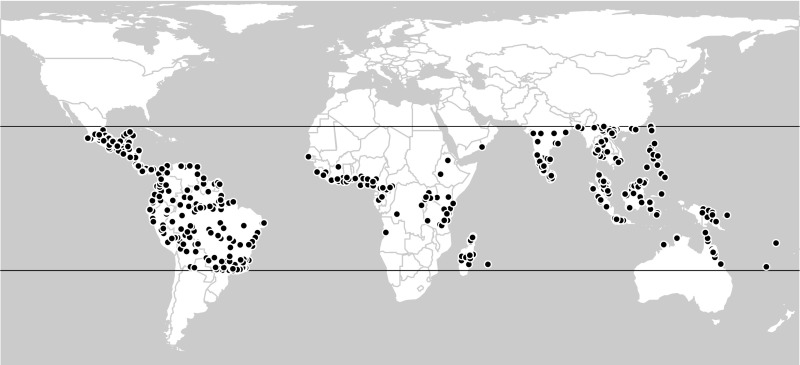
Fig. 1.

Spatial distribution of 875 tropical forest samples including either animals or trees that were drawn from the Ecological Register. The tropics of Cancer and Capricorn are indicated. The pattern mirrors the known distribution of field-based research campaigns in the tropics (19), but this dataset is more dispersed than the one used in a recent, related study (8) because the number of consulted references is greater (605 for the tropics alone vs. 284 for the globe).

Table S1.

Counts of samples used in this study by taxonomic group and altered habitat category

Group	Primary forest	Secondary forest	Lightly disturbed	Forest fragment	Plantation	Clearcut	Pasture	Cropland	Rural	Suburban	Urban	Total
Trees	57	10	26	3	1	—	—	—	—	—	—	97
Large mammals	32	7	9	1	5	—	—	2	1	—	—	57
Small mammals	46	10	6	7	8	2	5	6	3	1	2	96
Bats	60	23	4	6	4	—	3	6	3	1	5	115
Birds	44	19	10	5	12	—	1	1	1	—	—	93
Lizards	37	5	3	4	7	—	3	—	1	1	—	61
Frogs	56	6	4	2	8	—	5	2	1	—	—	84
Mosquitoes	25	4	2	3	4		4	9	13	5	4	73
Ants	32	8	3	8	8	—	1	3	—	—	1	64
Dung beetles	30	7	3	6	5	—	10	3	—	—	—	64
Butterflies	26	9	16	1	9	1	5	2	2	—	—	71
Total	445	108	86	46	71	3	37	34	25	8	12	875

All samples are from the tropical zone and from locations that were originally forested.

Instead of using sample data, global estimates of potential species extinction have tended to rely either on expert opinion (4) or on extrapolations that combine observed species–area relationships with expected or actual deforestation rates (e.g., refs. 1, 6). Actual extinctions are well-documented only for vertebrates (13). Even the underlying estimates of global diversity in certain groups have depended on indirect extrapolation methods of various kinds, such as scaling up from local-scale plot data (14) or from richness ratios between taxonomic levels (15). These methodologies yield disparate results and have individually come under strong criticism (15). With a few important exceptions (e.g., refs. 6–8, 16–18, and local-scale analyses reviewed in ref. 19), most researchers have also tended to focus on trees, mammals, birds, and a few other groups such as dung beetles (e.g., ref. 9). Finally, although important meta-analyses of local data have been carried out, most have used raw species-richness values (6, 7, 20), and no study has attempted to compare local and global species richness based on strictly comparable estimates that are controlled for sample-size effects.

Ecologists do make extensive use of methods that remove sampling biases, but such research has focused almost entirely on local samples. Many of these standardization analyses (8, 17, 18, 21) have used species counts interpolated to a least common denominator level by means of the long-established method of rarefaction (22, 23), which is problematic because rarefaction compresses differences between samples (24).

However, the compression problem can be solved using methods of either interpolation or extrapolation. Four different approaches are used in this paper (Methods). Two are analytical subsampling methods that seek to make samples comparable by drawing them down to the same completeness level based on expected counts of species sampled exactly once. One of these is called “shareholder quorum subsampling” (24) or “coverage-based rarefaction” (25), and the other is called “multiton subsampling.” The other two methods extrapolate the total number of species by considering counts of those found exactly once or twice. The first method (26), called “Chao 1” when applied to within-sample data and “Chao 2” when applied to among-sample incidence data, is very well-known (27). The second, called the “λ₅” or “lambda-5” extrapolator, has not been reported previously. Analyses presented in the main body of this text focus on the λ₅ method because it is particularly accurate when counts of individuals are uneven. However, global-scale Chao 1 and λ₅ estimates are extremely similar, and none of the results depend qualitatively on the choice of methods.

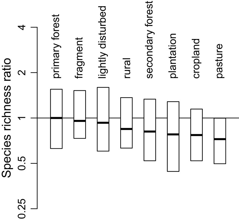
Disturbance has large effects at both local and global scales (Figs. 2, 3, and 4A and Tables S2 and S3). Local losses are >22% in pastures and croplands, and plantations and secondary forests are both >18% less rich than primary forests (Fig. 2 and Table S2). Indeed, although secondary forests are sometimes thought to foster high diversity (19), the data here suggest that they are nearly as depauperate as plantations (Fig. 2 and refs. 7 and 21). Just as surprisingly, forest fragments and forests disturbed by factors such as hunting, selective logging, and grazing are not significantly less rich than primary forests. Thus, although small protected areas are often valuable reservoirs of diversity, they are more effective when there is no history of intense tree removal.

Fig. 2.

Differences in species richness among habitat disturbance categories. The vertical axis is the ratio of the median local-scale richness value in a category to median richness in undisturbed (= primary) forests, as extrapolated using the λ₅ equation (Methods). Data are shown on a log scale. Each bar represents the interquartile range for all samples in a category, regardless of the group. Data are standardized before any other calculation by being divided by the group median. Only categories with at least 20 samples are illustrated (Table S1).

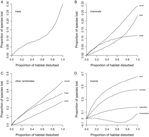
Fig. 3.

Expected species losses given varying amounts of habitat disturbance. The x axis is the proportion of randomly drawn samples that represent disturbed habitats; the y axis is the proportion of species expected to be lost. Underlying estimates are based on the λ₅ equation. (A) Trees. (B) Mammals. All large mammal species were sampled by camera traps; terrestrial species of small mammals were sampled using various kinds of traps. (C) Other vertebrates. (D) Insects.

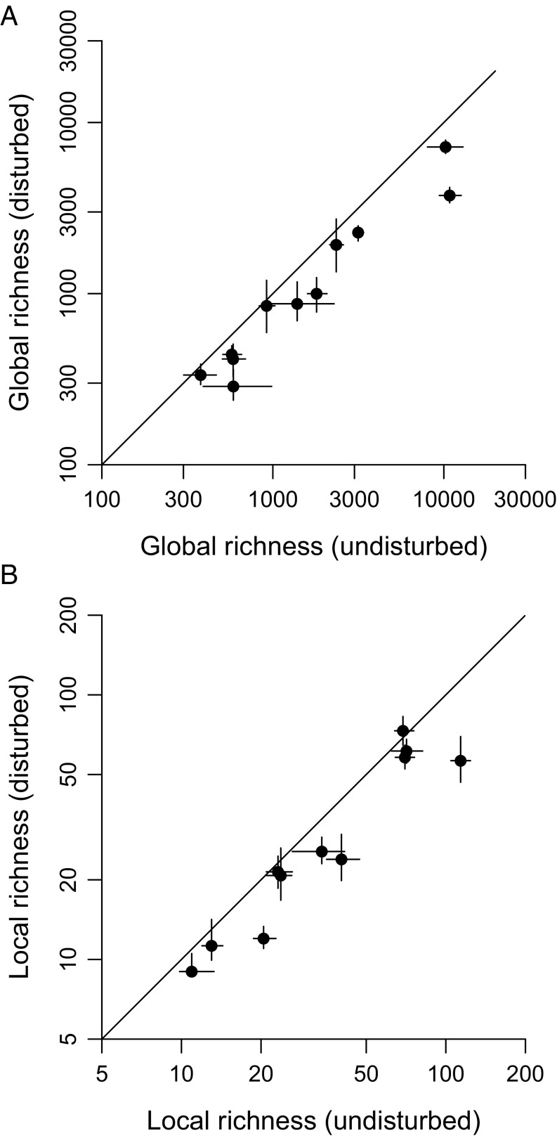
Fig. 4.

Effects of complete habitat disturbance on global and local richness of tropical species. Estimates are based on the λ₅ equation; similar patterns are produced by other methods (Figs. S3 and S4). Points are ecological groups. Lines through points indicate 95% CIs based on simultaneous resampling of samples and of species records within samples. Lines of unity are also shown. (A) Global richness in undisturbed and disturbed original forest environments. (B) Local richness in undisturbed and disturbed original forest environments.

Table S2.

Species richness losses by altered habitat category

Category	Samples	Effect size	P value
Primary forest	443	1	NA
Secondary forest	108	0.813	0.021
Lightly disturbed	86	0.930	0.400
Fragment	46	0.957	0.772
Plantation	71	0.778	0.006
Pasture	36	0.724	0.002
Cropland	34	0.771	0.033
Rural	25	0.845	0.226

Richness values are standardized using the λ₅ equation (Methods). Results are illustrated in Fig. 2. The effect size is the ratio of the median richness in a given category to the median richness in primary forests, also standardized for variation among taxonomic groups; the P value is the result of a Wilcoxon rank-sum test comparing primary forest values with the values in a given category. Ordering of columns follows Table S1. Categories with <20 samples are omitted.

Table S3.

Summary statistics regarding global richness estimates

Group	Undisturbed median	Disturbed median	Median ratio	Ratio lower CI	Ratio upper CI
Trees	10,241	7,195	0.703	0.547	0.914
Large mammals	378	335	0.884	0.691	1.153
Small mammals	586	415	0.706	0.536	0.909
Bats	575	441	0.769	0.649	0.908
Birds	3,153	2,277	0.721	0.630	0.810
Lizards	588	287	0.489	0.281	0.781
Frogs	1,388	872	0.631	0.364	1.027
Mosquitoes	919	849	0.923	0.632	1.321
Ants	10,820	3,748	0.346	0.288	0.418
Dung beetles	1,802	1,000	0.553	0.420	0.710
Butterflies	2,348	1,929	0.821	0.562	1.173

Median richness values are standardized using the λ₅ equation (Methods). The undisturbed median and the disturbed median are the median counts of species after bootstrapping within undisturbed and disturbed habitats. The median ratio is the median value of the ratios between bootstrapped counts. Ratio lower CI and ratio upper CI are the lower and upper bootstrapped CIs, which are respectively set at the 0.025 and 0.975 percentiles.

Increasing the level of disturbance would have strong effects on the global diversity of individual groups (Fig. 3). The term “global diversity” is used here to mean the overall richness estimate obtained by pooling all the local-scale species lists. Loss curves vary in shape in addition to scale, pointing to real biological differences among groups that have implications for conservation. The tree curve (Fig. 3A) is at first linear and then climbs steeply starting at about a 60–70% disturbance level, suggesting that there is a tipping point for this one group. The bat curve (Fig. 3B) is also somewhat exponential. Semiexponential curves are seen in simulation (SI Methods, Simulated Loss Curves) when species have relatively broad spatial distributions (Fig. S1 D–F). Asymptotic or linear trends are produced instead when geographic ranges are small relative to the scale of habitat disturbance (compare Fig. 3 B–D with Fig. S1 A–C). Thus, variation in curve shapes points to variation in range sizes among groups: Those exhibiting asymptotic trends presumably have smaller average extents and therefore are at greater risk of mass extinction. The simulation and empirical results also highlight the need to break up large-scale habitat disturbances by retaining fragments and corridors (SI Methods, Simulated Loss Curves). Finally, the negative values for mosquitoes at intermediate disturbance levels presumably reflect the invasion of disturbed forests by species adapted to open habitats, transiently increasing the size of the species pool. In any case, complete disturbance would ultimately lead to net species loss of mosquitoes. The overall implication is that any substantial loss of primary forests will result in numerous extinctions across many groups.

Fig. S1.

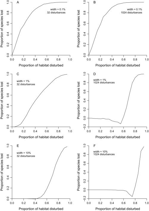
Simulated species losses given different amounts of habitat disturbance, different geographic range sizes, and different numbers of disturbance blocks. The x axis is the proportion of the geographic gradient that is disturbed, with no species surviving in disturbed blocks. Each panel legend indicates the width of the species ranges placed randomly across the unidimensional spatial gradient and the number of disturbance blocks, which are also randomly placed.

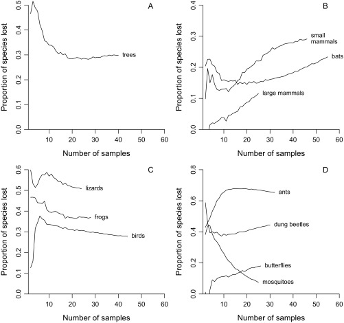
Indeed, expected global losses given complete disturbance are >18% in every single group except large mammals and mosquitoes and are >28% for seven groups in total (Figs. 3 and 4A and Table S3). The higher percentages generally apply to groups such as lizards and ants that have poor dispersal ability. Of concern, the various sampling biases discussed below might have depressed all the percentages. For example, the 30% estimate for trees (Table S3) combined with the fact that very few tree samples fall in moderately to highly disturbed categories (Table S1) suggests that this group is extinction resistant only in the sense that richness may be high in fragments and lightly disturbed forests. The only statistic that might well be liberal is the 28% figure for birds (Table S3). It should be interpreted cautiously because the sample data derive from mist-netting studies that typically capture small understory species, which might be more vulnerable to extinction (28). In any case, none of the results are strongly dependent on the number of samples used in the calculations except in the case of mosquitoes (Fig. S2). The mosquito trend (Fig. S2D) is consistent with there being no strong effect of disturbance on this group. Estimates for the three mammal categories are particularly conservative (Fig. S2B).

Fig. S2.

Expected species losses given complete habitat disturbance as a function of the number of samples used to the compute the λ₅ estimates. At each point on a given curve, the estimate is based on randomly drawing a fixed number of samples in each of the undisturbed and disturbed categories. (A) Trees. (B) Mammals. (C) Other vertebrates. (D) Insects.

Local-scale patterns are different, but they still broadly confirm the global-scale results (Fig. 4B and Table S4). In accord with the findings of multitaxon studies in individual systems (18) and with the global results (Fig. 4A), the local data suggest substantial differences among groups. One way or another, however, a large local footprint of disturbance is usually indicated (Table S4) because entirely pristine forests include more species (Fig. 2 and Table S2). The data for a few groups do fall close to the line of unity (Fig. 4B), indicating minor or even reversed local effects of disturbance: For example, butterfly richness is a little above the line (Table S4). However, ratios are far from unity for trees, frogs, and dung beetles. Regardless of such details, these local-scale results are in accord with the expectation that highly disturbed tropical forests are depauperate (6, 7, 29).

Table S4.

Summary statistics regarding average local richness estimates

Group	Undisturbed median	Disturbed median	Median ratio	Ratio lower CI	Ratio upper CI
Trees	113.7	56.4	0.497	0.405	0.618
Large mammals	23.8	20.8	0.878	0.679	1.154
Small mammals	10.9	9.0	0.851	0.688	1.012
Bats	23.2	21.4	0.926	0.765	1.106
Birds	70.0	58.1	0.829	0.725	0.949
Lizards	13.0	11.3	0.866	0.721	1.108
Frogs	20.5	12.0	0.584	0.511	0.661
Mosquitoes	34.0	25.6	0.754	0.598	0.996
Ants	71.0	61.3	0.862	0.729	1.026
Dung beetles	40.3	23.9	0.592	0.459	0.772
Butterflies	68.8	73.2	1.063	0.911	1.232

Median richness values are standardized using the λ₅ equation (Methods). See the legend of Table S3 for explanations of column headings.

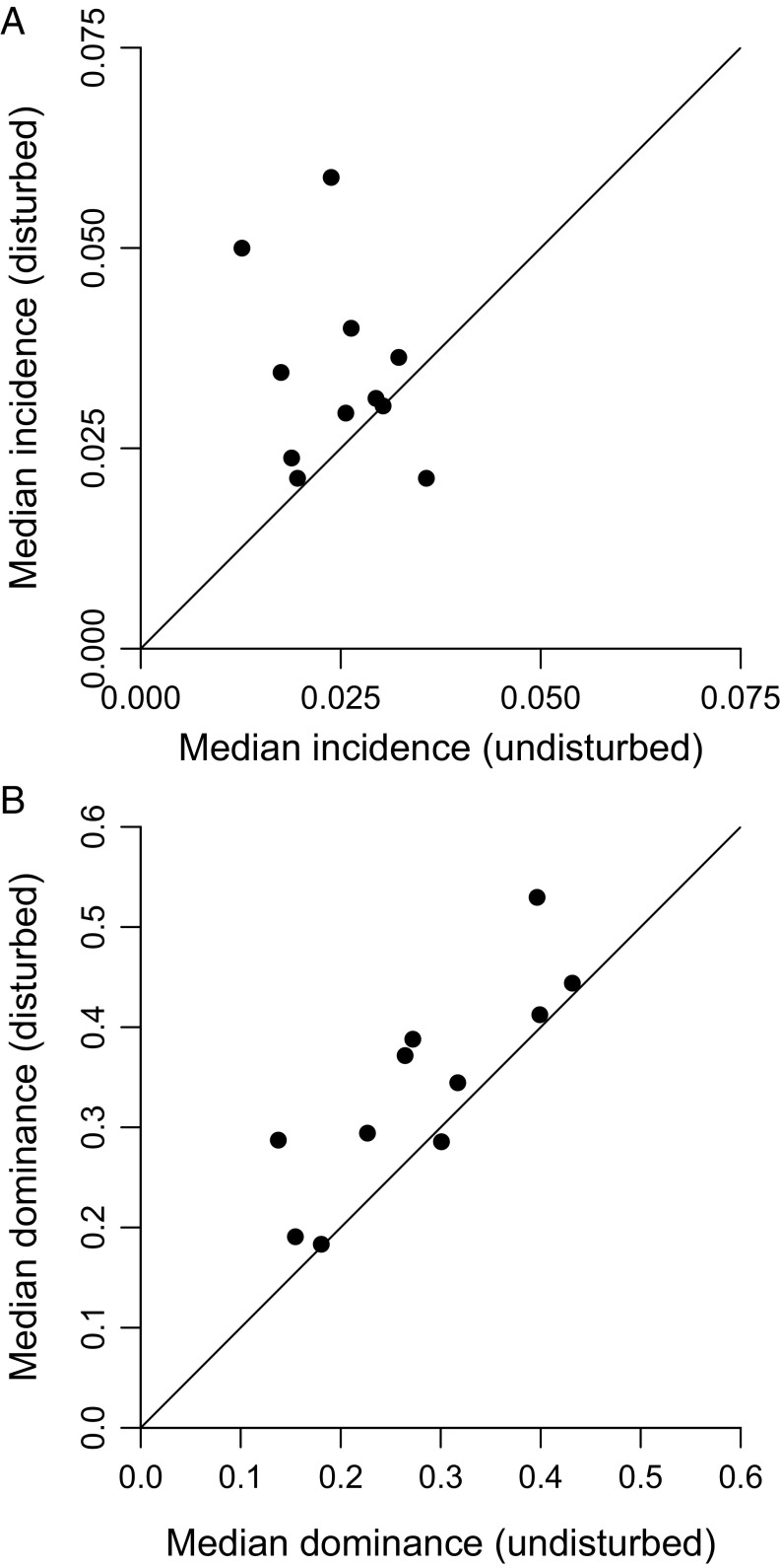
Weaker responses at local rather than global scales are counterintuitive but are easily explained by a simple mechanism: Disturbed ecosystems are dominated by widely dispersed, highly abundant, and often invasive species such as the pig (Sus scrofa), black rat (Rattus rattus), cane toad (Rhinella marina), southern house mosquito (Culex quinquefasciatus), electric ant (Wasmannia auropunctata), and globe skimmer (Pantala flavescens). This fact can be demonstrated by examining incidence proportions (frequencies of presence across samples), which in almost every group are higher on average in disturbed settings (Fig. 5A). Another useful measure is average dominance (the frequency of the most common species), which again shows a strong and consistent signal (Fig. 5B). Because high species losses at local scales are masked by the spread of common species able to tolerate human impacts, the most important results in this paper are those pertaining to potential extinction at the global scale.

Fig. 5.

Effects of complete habitat disturbance on species incidence and dominance within samples. Points are ecological groups. CIs are not shown because they would be minimal, given the large sample sizes. (A) Median incidence of species. Incidence is the proportion of samples that include a particular species. (B) Median dominance within samples. Dominance is the relative abundance of the most common species.

There are numerous reasons to believe that even the global estimates of richness loss are minimums. (i) Ecologists only infrequently study ecosystems that are highly unsuitable for the taxonomic groups of interest to them. Thus, the disturbed samples in this study tend to derive from suboptimal but still reasonably benign habitats. Indeed, only 10.7% of the samples (94 of 875) represent habitats that are completely deforested (Table S1). (ii) Many of the disturbed habitat samples (157, 17.9%) actually come from forests that are not strongly impacted (Fig. 2). This category includes rural forests, fragments, and lightly disturbed forests (those currently subjected to minor disturbance or described as being disturbed in a general way). (iii) Some nominal primary forest samples may be misclassified as such because of underreporting of contextual information in the primary literature that was consulted. (iv) Many disturbed samples are reported in the same papers as matched primary forest samples and therefore are spatially proximate to large tracts of nearly pristine habitat. Thus, individuals of rare species in disturbed habitats may have dispersed into them. (v) Some groups are actually more diverse in open habitats and therefore may prosper when primary forests are degraded (17, 18). (vi) The analyses reported here do not account for overall extinction debt [i.e., the fact that many surviving species will go globally extinct within the next few decades or centuries because their overall population sizes are not viable (29)]. Specifically, small populations in isolated forests will eventually be lost (30, 31), thus increasing the number of range-wide extinctions.

The most important point, however, is that many species may have already gone extinct because their ranges are now entirely deforested. These species were never in the sampling pools whose sizes have been estimated by extrapolating from the undisturbed habitat data. Furthermore, many species in otherwise pristine forests may have already gone extinct because of stressors not related to habitat destruction, such as hunting, interactions with invasive species, introduced epidemic diseases, pollution, and the direct effects of climate change. Thus, the current comparisons (Figs. 3 and 4) are between depauperate and very depauperate species pools. Given the rapid pace of deforestation throughout the tropics (10, 11), it therefore is conceivable that an event on the scale of a true mass extinction has already taken place. If recent, these losses may have gone unrecognized because the many rare species found in terrestrial communities are both at high risk of extinction and hard to sample on a regular basis. Regardless of this possibility, the current study paints a bleak picture of rapid, continuing loss of biodiversity even in a world where disturbed forests remain widespread.

Methods

Data.

The sample data used in this study were downloaded from the relational Ecological Register database (ecoregister.org) on 15 March 2017 using standard criteria, and these particular flat files have been archived at the same site (ecoregister.org/?page=data). Samples were defined as lists of species with matched abundances, as reported in the original literature. The datasets included as many published papers as possible. Only samples located between 23.44° N and 23.44° S and representing originally forested habitats were drawn. Woodland and savanna environments were excluded. Samples deriving from the same equal-area latitude/longitude degree cell, published in the same study, and representing the same original and altered habitats were lumped by summing the counts of individuals for each species.

Habitat alteration categories were similar to those used in a related study of strictly local-scale patterns (8), except that a unidimensional system was used instead of a two-way system with use intensity as the second axis. The reasons are that (i) the two axes are interdependent, with urban systems, for example, being “intense use” by definition; and (ii) extremely detailed information on use is not normally reported in the primary literature. Furthermore, secondary forests, forest fragments <100 ha in area, and lightly disturbed forests were split into separate categories instead of subsetting secondary forests by stand age (again, because detailed information on stand age is normally lacking). Clearcuts and rural and suburban settings were also recognized as separate categories. Forests were classified as being lightly disturbed if they were said to be disturbed in a general way or if they were subjected to grazing, selective logging, or hunting. Together, the additional categories capture the consistently recoverable information on use intensity.

Samples were divided into 11 primarily taxonomic groupings (Table S1). Tree samples were restricted to inventories based on a lower size cutoff of approximately 10-cm diameter at breast height. Large mammal samples were strictly derived from camera trapping studies; terrestrial small mammal studies were based on physical trapping studies; bat and bird samples were based on mist-netting; ant samples were based on pitfall and Winkler apparatus collections; and dung beetle samples were based on pitfall trapping. Specifically indeterminate records, which formed a small minority in most cases, were included in the analyses. If multiple records of indeterminate species stemmed from the same publication and were spelled identically, they were considered to represent a single morphospecies, whereas informal names spelled identically but stemming from different references were considered distinct. Counts of morphospecies are 5,239 (trees), 301 (large mammals), 380 (small mammals), 441 (bats), 2065 (birds), 332 (lizards), 787 (frogs), 811 (mosquitoes), 2,479 (ants), 815 (dung beetles), and 1,715 (butterflies).

Richness Estimation Methods.

Local analyses focused on counts of individuals within samples, whereas global analyses focused on counts of presences across samples. For example, if two samples respectively included species A and B and A and C, the respective presence counts would be 2, 1, and 1 for A, B, and C. Using presences in global analyses is standard procedure in the literature (e.g., ref. 24) and yields more accurate values in simulation.

Species richness was estimated using two extrapolation methods and two interpolation methods. The older extrapolation method (26) has two very similar variants, called the Chao 1 index when applied to raw counts of individuals and the Chao 2 index when applied to counts of presences. There are two names because a sample size correction term is used with presence counts. The basic form is S + s₀ = S + s₁²/2s₂ where S is the observed number of species, s₀ is the number of unsampled species, and s₁ and s₂ are the numbers of species respectively represented by exactly one or two individuals (i.e., the singletons and doubletons). Although the Chao indices assume that abundance distributions are nearly uniform, they are still well-established and widely used (27) and perform very well in simulation when this key assumption is met.

The second extrapolation approach seeks to account for the fact that real abundance distributions are typically far from uniform. It stems from reformulating Chao's equation in terms of Poisson sampling. Let λ be the average rate of sampling per species across the dataset. The chance of failing to draw a species is then e^−λ and that of drawing a singleton is λ e^−λ. If R is the unknown total number of species, then s₀ = R e^−λ and s₁ = R λ e^−λ. It follows that s₀/s₁ = 1/λ, λ = s₁/s₀, and s₀ = s₁/λ. A generic richness estimate therefore would be S + s₁/λ. Chao's equation can be justified on this account because it assumes that λ (here called “λ₁”) equals 2s₂/s₁, which is easily proven to be valid because s₂ = R λ² e^-λ/2. However, the value of λ can be fixed in a number of other ways by exploiting relationships such as S = R (1 − e^-λ) and N = R λ where N is the number of individuals. For example, we can define λ₂ = (N − s₁)/S and λ₃ = ln(N/s₁) and justify both by using simple algebra. Another easily proved estimator is λ₄ = −ln[s₁/λ₄ S(1 − e^−λ₄)], which can be computed recursively. It is interesting because it ignores N, but like all the estimators discussed to this point it is not particularly accurate.

The last estimator, λ₅, is the most complex and the most robust. It is computed by a simple hill-climbing equation from the equality ln[N/(S − s₁)] s₁/S = ln[λ/(1 − e^−λ − λ e^−λ)] λ e^−λ/(1 − e^−λ). Although daunting, this equation has intuitive components. First, like Chao 1, it implies that sampling is poor when s₁ is large (because s₁ appears by itself as a numerator and also in the denominator term S − s₁). Second, it implies that sampling is good when S is large (because S appears in two denominator terms). This idea makes sense because we eventually must encounter all species as S grows. Third, and most importantly, it implies that sampling is actually poor when N is large because large samples are likely to include some highly abundant species, so they should also include very rare species that are unlikely to be found. All the prominent species-abundance distributions such as the geometric series, log series, and log normal also rest on the assumption that when the most common species are very common, the rarest species are very rare. To put these considerations simply, the purpose of the N term is to compensate for the downward bias of most λ-based estimators that results from their assumption of uniformity in abundance.

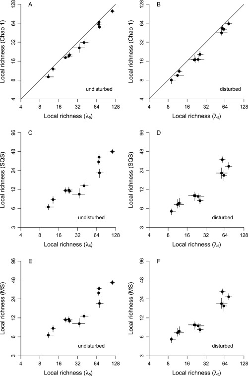
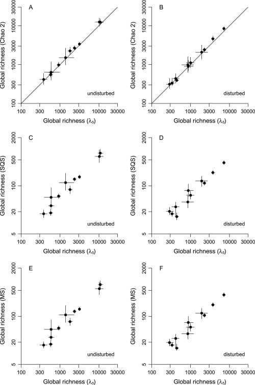
The λ₅ equation is emphasized throughout this paper because it outperforms all others in simulation by producing relatively unbiased estimates when abundances are very uneven. That said, the λ₅ method and the Chao indices do produce similar patterns when applied to the current data. The λ₅ estimates are a bit higher at the local scale, consistent with the expectation that this method will uncover more species when distributions are uneven but otherwise will yield the same values (Fig. 4B vs. Fig. S3A). Global-scale λ₅ estimates are slightly lower than Chao 2 estimates, but the differences are statistically insignificant for most groups (Fig. 4A vs. Fig. S4A). Values are more similar in this case because global presence–absence distributions tend to be quite flat and thus are more consistent with Chao 2's assumptions. The methods also yield very similar underlying richness estimates for the undisturbed and disturbed habitat categories at both scales (Figs. S5 A and B and S6 A and B).

Fig. S3.

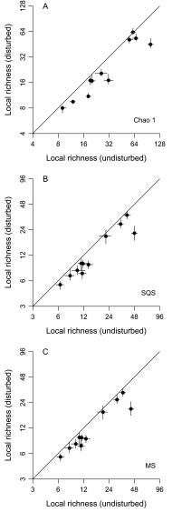
Effects of complete habitat disturbance on local richness, as estimated using three additional sampling standardization methods (compare with Fig. 4B). Values for undisturbed- and disturbed-habitat samples are shown on the x and y axes, respectively. Points are ecological groups, and lines through points indicate 95% CIs. Lines of unity are shown. (A) Chao 1. (B) Shareholder quorum subsampling (SQS, a.k.a. coverage-based rarefaction) with a quorum of 0.90. (C) Multiton subsampling with a target of 4.

Fig. S4.

Effects of complete habitat disturbance on global richness, as estimated using three additional sampling standardization methods (compare with Fig. 4A). See the legend of Fig. S3 for additional details. (A) Chao 2. (B) Shareholder quorum subsampling (a.k.a. coverage-based rarefaction) with a quorum of 0.10. (C) Multiton subsampling with a target of 0.05.

Fig. S5.

Comparisons of local richness estimates generated by the λ₅ equation (x axes) and three other methods (y axes, with each method corresponding to a row). Separate estimates for samples from undisturbed habitats (Left) and from disturbed habitats (Right) are given. Points are ecological groups, and lines through points indicate 95% CIs. Lines of unity are shown only for Chao 1 because the other methods work through interpolation instead of extrapolation, so average values are not comparable to λ₅ values. Shareholder quorum subsampling quorums are 0.90, and multiton targets are 4. (A) Chao 1 (undisturbed data). (B) Chao 1 (disturbed data). (C) Shareholder quorum subsampling (undisturbed data). (D) Shareholder quorum subsampling (disturbed data). (E) Multiton subsampling (undisturbed data). (F) Multiton subsampling (disturbed data).

Fig. S6.

Comparisons of global richness estimates generated by the λ₅ equation (x axes) and three other methods (y axes). Shareholder quorum subsampling quorums are 0.10, and multiton targets are 0.05. See the legend of Fig. S5 for additional details. (A) Chao 2 (undisturbed data). (B) Chao 2 (disturbed data). (C) Shareholder quorum subsampling (undisturbed data). (D) Shareholder quorum subsampling (disturbed data). (E) Multiton subsampling (undisturbed data). (F) Multiton subsampling (disturbed data).

The first subsampling method was originally called “shareholder quorum subsampling” (24) and is now often called “coverage-based rarefaction” (25). It was originally an algorithmic approach (24), but calculations here are based on exact equations (25). Its goal is to determine the expected richness at a certain sampling level such that Good's index of frequency distribution coverage equals a fixed target, called a “quorum” (24). The index is 1 − s₁/N. The second subsampling method is also analytical and is called “multiton subsampling” (SI Methods, Multiton Subsampling). It is based on examining the ratio (S − s₁)/S where S − s₁ is the number of nonsingletons (i.e., multitons). To guarantee that it will rise monotonically with N, the observed ratio at a candidate sampling level N_i is multiplied by N_i/(s_1,i +1) where s_1,i is a candidate singleton count. An exact algorithm is used to find subsampled richness given a desired (target) multiton ratio.

The end-member richness ratios generated by the λ₅ equation (Fig. 4) are similar to those produced by the two interpolation methods (Figs. S3 B and C and S4 B and C). That said, the underlying values are substantially different (Figs. S5 C–F and S6 C–F). Again, the λ₅ results are emphasized in this paper because this method builds in an explicit correction for the unevenness of abundance distributions, but the other three do not.

Loss Curves.

In the analyses varying the proportions of undisturbed and disturbed samples (Fig. 3), each illustrated species loss value equals 1 − S_d/S_u where S_d represents the number of species estimated to remain at a given disturbance level and S_u represents the estimated number given no disturbance. The global estimate S_d at each level reflects a mixture of disturbed and undisturbed local samples. For example, at one extreme all samples are undisturbed, so S_d = S_u; at the other all are undisturbed; and at the midpoint 50% are in each category. The combined number of samples drawn at each step was fixed, with the quota equaling the smaller of the total counts in each category. Quotas were 40 samples (trees), 25 (large mammals), 46 (small mammals), 55 (bats), 44 (birds), 24 (lizards), 28 (frogs), 25 (mosquitoes), 32 (ants), 30 (dung beetles), and 26 (butterflies). To compute an individual S_d value, an appropriate number of samples in each category was drawn at random; the species list for each sample was bootstrapped (i.e., sampled with replacement); the presences were summed; and a global richness estimate for the combined presences was computed using the λ₅ equation. Each point in a given curve represents the median 1 − S_d/S_u value generated by 10,000 randomization trials.

CIs on Local Richness Estimates.

The CIs (Fig. 4B and Figs. S3 and S5) were computed using a two-layer bootstrapping protocol. First, during each of 1,000 trials each sample's species list was bootstrapped up to the original richness level; the randomized abundances were used to obtain a richness estimate by means of the appropriate method; and the median richness across samples was found. Separate distributions of medians were computed for the disturbed and undisturbed data partitions. Second, the medians for the disturbed samples were sampled with replacement 10,000 times; the same was done with the undisturbed sample medians; the ratio of the two vectors was taken; and nonparametric CIs (based on percentiles) were then computed using the ratio vector. Because the CIs are nonparametric, some are seen to be asymmetrical in Fig. 4B.

CIs on Global Richness Estimates.

Calculations similar to those used in the loss-curve analysis were used to obtain CIs for the global-scale data (Fig. 4A and Figs. S4 and S6). First, during each of 10,000 trials the list of samples itself was sampled without replacement down to the least common denominator level for the two disturbance categories (i.e., the relevant quota given in the list above). Because of computational limits, 1,000 trials were carried out when applying the two subsampling methods instead of the two extrapolation methods. Second, during each trial all the drawn samples in a given category were transformed to presences and summed; estimates were made using the four methods; and the standardized richness values were recorded in arrays. Third, the arrays of 10,000 richness values in each category were sampled with replacement 10,000 times, and the ratios were recorded. Finally, nonparametric CIs were computed from those data.

Incidence and Dominance Calculations.

Incidence (Fig. 5A) was computed by taking the ratio of the number of samples including a given species (X_i) to the total number of samples representing the relevant group (X). However, raw ratios are somewhat upward biased when X is small because they have a lower bound of 1/X. Thus, a mild correction was used: X was incremented by 1 to produce the ratio X_i(X + 1). This correction had no qualitative effect on the results. CIs on across-species medians are not shown because the extremely large sample sizes render them too small to illustrate meaningfully.

Dominance figures were computed directly from the species abundance data for the individual samples, with each sample yielding a single dominance value equal to the maximum abundance of any included species divided by the sum of abundances. Again, CIs are not illustrated (Fig. 5B) because sample sizes are so large.

SI Methods

Simulated Loss Curves.

Differences in the shapes of loss curves (Fig. 3) can be accounted for by a simulation model making very simple assumptions. It supposes that each of 100 species occupies a narrow, continuous, randomly centered range across a unidimensional spatial gradient (as opposed to having many local populations that are distributed across the entire gradient). The width of each distribution is set at 0.1, 1, or 10% of the gradient, depending on the scenario. One hundred local samples are placed randomly along the gradient, and local sampling is assumed to be complete. Equal-width disturbance blocks are randomly placed on the gradient, and all species are removed from all samples falling within these blocks. Either 32 blocks or 1,024 blocks are placed. The width of the blocks is back-computed from the desired proportion of the gradient to be disturbed. For example, if 10% is to be disturbed and 32 blocks are to be placed, the blocks need to be 1–0.9^1/32 = 0.0033 gradient units wide, and placing them end-to-end instead of randomly would erase 10.5% of the gradient. To mimic the empirical analyses, the number of species in the system is extrapolated from the observed presence–absence distribution using the λ₅ equation. The estimated number of species at each disturbance level in a given scenario is recorded to produce a loss curve, and the entire procedure is iterated 1,000 times.

Because the number of samples is finite and the sampling regime is artificial, the λ₅ estimates are not always exactly correct. Therefore, the curve is rescaled to range from 0 to 1, with the curve's starting value equating to 0. For example, if the λ₅ richness estimate is 100 species with no disturbance and 30 with 50% disturbance, the curve rises from 0 to 0.7 at the latter point. The same scaling procedure was used to create the empirical curves (Fig. 3).

This simple model easily accounts for the major patterns seen in Fig. 3. Asymptotic trends are seen when species have very narrow geographic range sizes (Fig. S1 A and B). In other words, extinction proceeds quickly when species are highly endemic, as one might expect. Linear patterns of the kind seen for several groups (Fig. 3) arise only when species have medium-sized ranges (1% of the gradient) and disturbance blocks are large (Fig. S1C). Semiexponential trends are seen in all other cases (Fig. S1 D–F). These threshold patterns arise when disturbances are very localized relative to range sizes, either because ranges are large (Fig. S 1 E and F) or because disturbance is very fine-grained (Fig. S1 D and F). In either circumstance it is difficult to cause extinctions without erasing a large fraction of all available habitat.

The tendency of the trends based on subsampling to be linear or asymptotic (Fig. 3) is therefore realistic because most species do inhabit relatively small regions when considered on a global scale. To put this assertion in perspective, it is worth noting that 1% of the surface of the continents amounts to an area roughly the size of Peru. Thus, the most realistic simulation scenarios might be the ones in which ranges are on the order of 0.1% of the available area (Fig. S1 A and B), in which cases we might expect disturbed areas to be relatively large compared with the range sizes of many species. If these assumptions are wrong, and disturbance blocks in the real world do tend to be smaller than range sizes (Fig. S1 D–F), then we might expect more groups to exhibit tipping point behavior in the future.

A minor note: The loss curves decline transiently below zero in two scenarios that both involve fine-scale disturbance with range sizes exceeding block sizes (Fig. S1 D and F). This behavior results from overestimation of richness just before tipping points are reached, possibly because the number of single-sample species exceeds any reasonable expectation derived from Poisson sampling theory when range fragmentation is extreme. The exact cause is unclear, but the pattern provides no real reason to think that λ₅ suffers from a large systematic bias because the circumstances are so narrow.

In any event, the simulation results make it clear that to avoid rapid extinction it is essential to narrow the local extent of disturbances. At least on a theoretical level, mosaic landscapes with many small fragments are preferable to landscapes with small numbers of large fragments. Meanwhile, the simulations suggest that the possibility of a major mass extinction of organisms with small ranges already having occurred must be considered in light of the spatial grain of disturbance. Quantifying disturbance scales and comparing them to historical range size data would be an avenue for future research.

Effect of Sample Size.

Like anything else, extrapolation using the λ₅ equation (Methods) is expected to work poorly when sample sizes are very limited. The open question is whether the datasets used in this study are large enough to constrain the pool size estimates used to infer the effects of habitat disturbance on global richness (Figs. 3 and 4A). If so, we should expect to see a plateau in the relationship between the amount of data drawn and the proportion of species estimated to be lost.

To make such an analysis possible, the numbers of undisturbed and disturbed samples must be made to match at any given level of sampling. In other words, a single quota on the size of each partition must be imposed. This requirement must be met even when using as much data as possible. The quotas that result from this consideration are applied here both to the analysis contrasting amount of disturbance with species loss (Fig. 3) and to the analysis projecting loss given complete disturbance (Fig. 4A), which is simply the end-member case (compare Fig. 4A with end points of curves in Fig. 3).

Fig. S2 illustrates the effect of gradually increasing the quotas from the logical minimum (two) to the maximal values actually used in the rest of the study. The x axis is the quota, i.e., the number of samples in each of the undisturbed and disturbed categories. At each point on a curve, the loss value is one minus the ratio of the richness estimate based on the disturbed samples to the estimate based on the undisturbed samples. For example, if the disturbed and undisturbed samples respectively yield estimates of 1,000 and 4,000 species, the expected loss is 1–1,000/4,000 = 0.75. The values are medians across 10,000 bootstrapping trials, with each trial following the same procedure used in the related analyses of Figs. 3 and 4A: A set of samples is first drawn from the master list, and then the individual samples are individually bootstrapped by sampling the species with replacement.

The resulting curves suggest that sample size effects are weak to absent in most groups. A fairly obvious plateau is seen in the curve for trees (Fig. S2A). There are weak downward or upward trends for many of the other groups, but it is possible that asymptotes are not far off in these cases. There are stronger upward trends for bats and especially for large mammals (Fig. S2B), and the data for dung beetles and butterflies (Fig. S2D) are equivocal. However, these data are not a problem because the trends are conservative relative to the main claim made in this paper: that further habitat disturbance can be expected to cause unexpectedly large losses. The only pattern of substantial concern is a strong decrease for mosquitoes (Fig. S2D). However, projected losses are so small for this group that the exact figures hardly matter. The important point is that none of the other curves end anywhere close to zero.

Multiton Subsampling.

Shareholder quorum subsampling (24), also called “coverage-based rarefaction” (25), has come into wide use because it largely solves the problem of richness estimate compression: If two samples differ in underlying, actual richness by a factor of two, it will generally find that the richness ratio is two no matter what the desired interpolation level (24). The method involves drawing down the data to a fixed level of frequency distribution coverage as defined using Good's equation (32), i.e., 1 − s₁/N where s₁ is the number of singletons and N is the number of individuals. Quorum subsampling can implemented either algorithmically (24, 33) or using an exact analytical equation (25).

In this section, I discuss a newer, also analytical method, multiton subsampling, that yields similar results but is more robust. It involves computing expected richness given a specified ratio or “target” equal to (S − s₁)/S where S is the total number of species and S − s₁ is the number of species represented by at least two individuals in a sample (the multitons).

To obtain an estimate, different potential sample sizes, N_i, in terms of the number of individuals are considered; for each N_i, the expected numbers of species overall and of singletons are computed using standard combinatorial equations (23, 25); and expected richness is computed as the average species count yielded by the two N_i counts, yielding multiton ratios that straddle the target. Samples then can be compared by finding their expected richness levels, given that all have been drawn down to the same target.

At very low sample sizes, more than one N_i value might produce the same (S − s₁)/S ratio, violating the intuitive principle that a sampling quality measure should rise monotonically with the amount of raw data. This problem is easily resolved by multiplying the target ratio by N_i/(s_1,i + 1) where s_1,i is the number of singletons expected to be found in a sample of size N_i. The target then is a positive number potentially >1 instead of a proportion ranging from 0 to 1.

Global data for all groups are analyzed at a target multiton ratio of 0.05, and local data are analyzed at a target ratio of 4. Both values take the aforementioned scaling term into account. The targets were selected as the lowest common denominator values across ecological groups. The global figure is low because global presence–absence distributions are extremely flat. The equivalent quorum subsampling targets are 0.10 (global data) and 0.90 (local data). These figures were selected to make sure that the absolute values returned by the two methods would be roughly comparable.

The multiton method is similar to shareholder quorum subsampling in that both uncompress the data. The two also yield highly correlated results (Figs. S5 A and B and S6 A and B). The difference is that the older method produces values that are less precise and substantially more biased, especially when richness is either very low or very high.

References

- 1.Sala OE, et al. Global biodiversity scenarios for the year 2100. Science. 2000;287:1770–1774. doi: 10.1126/science.287.5459.1770. [DOI] [PubMed] [Google Scholar]
- 2.Brooks TM, et al. Habitat loss and extinction in the hotspots of biodiversity. Conserv Biol. 2002;16:909–923. [Google Scholar]
- 3.Laurance WF, et al. Averting biodiversity collapse in tropical forest protected areas. Nature. 2012;489:290–294. doi: 10.1038/nature11318. [DOI] [PubMed] [Google Scholar]
- 4.Feeley KJ, Silman MR. Biotic attrition from tropical forests correcting for truncated temperature niches. Glob Change Biol. 2010;16:1830–1836. [Google Scholar]
- 5.Huey RB, et al. Why tropical forest lizards are vulnerable to climate warming. Proc Biol Sci. 2009;276:1939–1948. doi: 10.1098/rspb.2008.1957. [DOI] [PMC free article] [PubMed] [Google Scholar]
- 6.Chaudhary A, Burivalova Z, Koh LP, Hellweg S. Impact of forest management on species richness: Global meta-analysis and economic trade-offs. Sci Rep. 2016;6:23954. doi: 10.1038/srep23954. [DOI] [PMC free article] [PubMed] [Google Scholar]
- 7.Gibson L, et al. Primary forests are irreplaceable for sustaining tropical biodiversity. Nature. 2011;478:378–381. doi: 10.1038/nature10425. [DOI] [PubMed] [Google Scholar]
- 8.Newbold T, et al. Global effects of land use on local terrestrial biodiversity. Nature. 2015;520:45–50. doi: 10.1038/nature14324. [DOI] [PubMed] [Google Scholar]
- 9.Barlow J, et al. Anthropogenic disturbance in tropical forests can double biodiversity loss from deforestation. Nature. 2016;535:144–147. doi: 10.1038/nature18326. [DOI] [PubMed] [Google Scholar]
- 10.Kim D-H, Sexton JO, Townshend JR. Accelerated deforestation in the humid tropics from the 1990s to the 2000s. Geophys Res Lett. 2015;42:3495–3501. doi: 10.1002/2014GL062777. [DOI] [PMC free article] [PubMed] [Google Scholar]
- 11.Leisher C, Touval J, Hess SM, Boucher TM, Reymondin L. Land and forest degradation inside protected areas in Latin America. Diversity (Basel) 2013;5:779–795. [Google Scholar]
- 12.Rodrigues ASL, et al. Effectiveness of the global protected area network in representing species diversity. Nature. 2004;428:640–643. doi: 10.1038/nature02422. [DOI] [PubMed] [Google Scholar]
- 13.Dirzo R, et al. Defaunation in the Anthropocene. Science. 2014;345:401–406. doi: 10.1126/science.1251817. [DOI] [PubMed] [Google Scholar]
- 14.Wilson JB, Peet RK, Dengler J, Pärtel M. Plant species richness: The world records. J Veg Sci. 2012;23:796–802. [Google Scholar]
- 15.Mora C, Tittensor DP, Adl S, Simpson AGB, Worm B. How many species are there on Earth and in the ocean? PLoS Biol. 2011;9:e1001127. doi: 10.1371/journal.pbio.1001127. [DOI] [PMC free article] [PubMed] [Google Scholar]
- 16.Lawton JH, et al. Biodiversity inventories, indicator taxa and effects of habitat modification in tropical forest. Nature. 1998;391:72–76. [Google Scholar]
- 17.Schulze CH, et al. Biodiversity indicator groups of tropical land-use systems: Comparing plants, birds, and insects. Ecol Appl. 2004;14:1321–1333. [Google Scholar]
- 18.Barlow J, et al. Quantifying the biodiversity value of tropical primary, secondary, and plantation forests. Proc Natl Acad Sci USA. 2007;104:18555–18560. doi: 10.1073/pnas.0703333104. [DOI] [PMC free article] [PubMed] [Google Scholar]
- 19.Gardner TA, et al. Prospects for tropical forest biodiversity in a human-modified world. Ecol Lett. 2009;12:561–582. doi: 10.1111/j.1461-0248.2009.01294.x. [DOI] [PubMed] [Google Scholar]
- 20.Dunn RR. Recovery of faunal communities during tropical forest regeneration. Conserv Biol. 2004;18:302–309. [Google Scholar]
- 21.Gardner TA, Hernández MIM, Barlow J, Peres CA. Understanding the biodiversity consequences of habitat change: The value of secondary and plantation forests for neotropical dung beetles. J Appl Ecol. 2008;45:883–893. [Google Scholar]
- 22.Sanders HL. Marine benthic diversity: A comparative study. Am Nat. 1968;102:243–282. [Google Scholar]
- 23.Hurlbert SH. The nonconcept of species diversity: A critique and alternative parameters. Ecology. 1971;52:577–586. doi: 10.2307/1934145. [DOI] [PubMed] [Google Scholar]
- 24.Alroy J. The shifting balance of diversity among major marine animal groups. Science. 2010;329:1191–1194. doi: 10.1126/science.1189910. [DOI] [PubMed] [Google Scholar]
- 25.Chao A, Jost L. Coverage-based rarefaction and extrapolation: Standardizing samples by completeness rather than size. Ecology. 2012;93:2533–2547. doi: 10.1890/11-1952.1. [DOI] [PubMed] [Google Scholar]
- 26.Chao A. Non-parametric estimation of the number of classes in a population. Scand J Stat. 1984;11:265–270. [Google Scholar]
- 27.Walther BA, Moore JL. The concepts of bias, precision and accuracy, and their use in testing the performance of species richness estimators, with a literature review of estimator performance. Ecography. 2005;28:815–829. [Google Scholar]
- 28.Sodhi NS, et al. Perspectives in ornithology: Effects of disturbance or loss of tropical rainforest on birds. Auk. 2008;125:511–519. [Google Scholar]
- 29.Tilman D, May RM, Lehman CL, Nowak MA. Habitat destruction and the extinction debt. Nature. 1994;371:65–66. [Google Scholar]
- 30.Turner IM. Species loss in fragments of tropical rain forest: A review of the evidence. J Appl Ecol. 1996;33:200–209. [Google Scholar]
- 31.Brooks TM, Pimm SL, Oyugi JO. Time lag between deforestation and bird extinction in tropical forest fragments. Conserv Biol. 1999;13:1140–1150. [Google Scholar]
- 32.Good IJ. The population frequencies of species and the estimation of population parameters. Biometrika. 1953;40:237–264. [Google Scholar]
- 33.Alroy J. Accurate and precise estimates of origination and extinction rates. Paleobiology. 2014;40:374–397. [Google Scholar]