

Abstract
The paper introduces an algorithm which allows the automatic segmentation of multi channel magnetic resonance images. We extended the Expectation Maximization-Mean Field Approximation Segmenter, to include Local Prior Probability Maps. Thereby our algorithm estimates the bias field in the image while simultaneously assigning voxels to different tissue classes under prior probability maps. The probability maps were aligned to the subject using nonrigid registration. This allowed the parcellation of cortical sub-structures including the superior temporal gyrus. To our knowledge this is the first description of an algorithm capable of automatic cortical parcellation incorporating strong noise reduction and image intensity correction.
1 Introduction
Quantitative medical image analysis often involves segmentation to assess the shape and volume of anatomical structures. Progress has been made for major tissue classes, however, segmentation of other structures is still difficult. Manually segmenting hundreds of cases is not only time consuming but also has large variations. Given these factors, the need for automatic and validated segmentation methods is clear.
There are several approaches to achieve this goal. The Level Set Method introduced by Osher and Sethian [1] segments images by evolving predefined shapes to fit the image. Leventon [2], Tsai [3] and Baillard [4] introduced this method to the clinical field by using complex anatomical information. These methods ignore the intra-scan inhomogeneities, often caused by the radio-frequency (RF) coils, or acquisition sequences. Comprehensive validation studies are still needed regarding these methods.
Using registration for segmentation is another approach. These methods use a previously segmented brain and align it with the subject. The result of this alignment is the segmentation. Fischl et el. [5] uses a detailed atlas with over 30 different labels to segment the brain. The ANIMAL+INSECT algorithm [6] on the other hand uses two algorithms at the same time. The ANIMAL is responsible for the non-rigid alignment of an atlas with the subject. The INSECT corrects the intensity inhomogeneity in the image. Nevertheless, segmentation by registration approaches cannot segment structures, which are not projected from the atlas onto the subject. For example, white matter lesions, which are common in several neurological diseases, cannot be identified with such an approach. As an alternative, some algorithms have been proposed which combine intensity based classification with segmentation by registration (Warfield [7]).
A very different approach introduced to the medical field by Wells [8], is the Adaptive Segmentation, which uses an Expectation Maximization (EM) Algorithm. It simultaneously labels and estimates the intensity inhomogeneities artifacts in the image. To add more robustness through noise rejection, Kapur [9] incorporated the Mean-Field Approximation (MF) for the labeling mechanism. However, the algorithm lacked any shape information. Van Leemput [10] improved this handicap by including prior probability maps (PPM) of tissue class spatial distribution into the initial formulation of Wells togther with a MF. He used affine registration to align PPMs with the subject. He iteratively updated the tissue class distributions and the labeling of the image simultaneously. To date, the published results indicate that ‘the method may occasionally fail, due to poor initialization … This problem may be overcome by using non rigid rather than affine registration for matching.’ [10] Additionally Van Leemput did not consider parcellation of the cortex.
Like Van Leemput, we used the Expectation Maximization-Mean Field Approximation (EM-MF) Algorithm for the segmentation itself, however, we align the PPM through non-rigid registration. Compared to registration alone, this approach has the advantage of segmenting tissue classes relative to each other. Therefore, it can better cope with large artifacts in the image, such as significant intensity differences between the subject and the atlas. It allows us to parcellate substructures of the cortex, e.g. amygdala or parrahippocampal gyrus. We demonstrate the clinical usefulness of our new algorithm by carrying out validation experiments on the task of superior temporal gyrus (STG) segmentations.
2 Method
As mentioned, the Expectation Maximization - Mean Field Approximation - Local Prior Algorithm (EM-MF-LP) first registers PPMs to the subject. The method then uses the EM-MF algorithm, defined through Expectation-Step (E-Step) and Maximization-Step (M-Step), to segment the subject. The E-Step is responsible for calculating the weights, representing the likelihood of tissue classes, using the aligned PPMs. The M-Step calculates the bias field, which models the intensity inhomogeneity artifact. These two steps are repeated until the algorithm converges.
The PPMs used in this paper were derived from 82 different subjects using a statistical atlas construction method described by Warfield [11]. This method projects anatomy from a source to a target, such as white matter from subject a to subject b. The result is a minimum entropy anatomical model and a statistical volume or probability map for each tissue class.
2.1 Non-rigid Registration
In order to use these PPMs, we must register them to our subject. We register the SPGR corresponding to the target of the statistical atlases to the subjects SPGR, and project the PPMs using the same transformation. To do so, we use a deformable registration procedure [12, 13]. It finds the displacement v(x) for each voxel x of a target image T to match the corresponding anatomical location in a source image S. The solution is found using the following iterative scheme:
| (1) |
where Gσ is a Gaussian filter with a variance of σ2, ⊗ denotes convolution, ○ denotes the composition, ∇ is the gradient operator and the transformation h(x) is related to the displacement v(x) by h(x)=x+v(x). is an intensity corrected version of S computed at the nth iteration to help capture intensity variations present between the images to register.
Equation (1) finds voxel displacements in the gradient direction . Convolution with a Gaussian kernel Gσ is performed to model a smoothly varying displacement field. As is common with registration methods, multi-resolution techniques are used to accelerate convergence.
2.2 EM-MF
When segmenting magnetic resonance images (MRI) it is hard to determine the inhomogeneities without knowing the tissue type of every voxel. On the other hand, one cannot find out the tissue type without knowledge of the inhomogeneities. Therefore, the adaptive segmentation approach [8] will try to solve for these two unknowns simultaneously.
In the Expectation Step (E-Step), the algorithm calculates the expected value of the weight (also see Kapur [9])
| (2) |
where Y(x,y,z) is the log intensity and β(x,y,z) is the bias of the image at voxel (x,y,z), T is the tissue class, DT is the tissue class distribution, and N is the normalizing factor of weight WT. The energy function ET (x,y,z), representing the mean field approximation, is defined as
| (3) |
where M is the number of classes, U = U(x,y,z) is the neighborhood of (x,y,z) and
| (4) |
is the ‘Tissue Class Interaction Matrix’ (CIM).
The Maximization Step (M-Step) calculates the maximum a-posteriori (MAP) estimate of the bias field assuming the weight calculation in the previous step is correct for every voxel.
| (5) |
where is the mean residual, defined by DT, and Y, and H is determined by the mean tissue class covariances and the bias covariance (see Wells [8]).
2.3 The EM-MF-LP
The EM-MF Algorithm, described in Section 2.2, assumed that the probability for a given tissue class P(T) does not change throughout the image. For the EM-MF-LP algorithm this assumption will be dropped. P(T), in equation (2), will be substituted with P(T|x,y,z). Thus the weight in the E-Step will be updated as follows:
| (6) |
The EM-MF-LP Algorithm works in two phases (see Figure 1). First, it registers the brain atlas with the subject. The resulting deformation field is used to align the PPMs to the subject. The aligned PPMs define the local prior probability P(T|x,y,z). In the second phase, it segments the image using EM-MF Algorithm with the updated E-Step (see Equation 6).
Fig. 1.
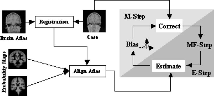
The structure of the EM-MF-LP Algorithm
3 Implementation and Experiments
The algorithm is fully integrated in the 3D Slicer [14], which is a software package for medical image analysis. A basic version of the described method is publicly available at http://www.slicer.org. The user interface guides the user through the segmentation process. Tissue definitions for the actual image can be done manually or automatically. Graphs and other tools help to verify the results.
To show the improvements of the EM-MF-LP method over other approaches, the different strategies will be compared on one MRI Scan with 256×256 pixels. Both Spoiled Gradient Recalled Acquisitions in the Steady State(SPGR) and T2 weighted intensity features were. The resulting segmentations are displayed in Figure 2. The first method is simply using brain mapping with non-rigid Registration (NRR). After the atlas brain is registered with the subject, the PPMs are then aligned. Each voxel is assigned to the tissue class with the highest a posteriori probability. This approach is very similar to Fischl[5], Pachai[15], and Collins[6]. The segmentation is only a rough estimate, which is too ’stiff’ for the subject. Especially the CSF at the outside of the brain is underestimated.
Fig. 2.
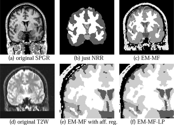
Segmenting up to 7 tissue classes with different methods. Methods used in (b) and (c) do not allow the parcelation of cortical substructures. In (e) the misclassifcation of the scalp is visible as described in [10]. These errors are eliminated in our result shown in(f).
The EM-MF Algorithm is more flexible than NRR (see Figure 2(c)). In addition, the algorithm better incorporates the image inhomogeneities. However, voxels are still seen independently, which causes additional noise. Segmenting cortical substructures is not possible, as opposed to NRR. Again, the need for increased usage of spatial information is very apparent. In Figure 2(f), we use the method described in Section 2. Figure 2(e) is the same method, but the non-rigid registration is substituted with an affine one, similar to Van Leemputs’ approach. Comparing 2(e) to 2(f) the dangers of including local priors into the EM-MF Algorithm are readily apparent. The STG in Figure 2(e) is expanding into neighboring structures like the middle temporal gyrus. Also as in Van Leemput’s paper [10] additional misclassification at the outside of the brain can be observed in Figure 2(e). This is primarily due to poor alignment of the atlases. It can readily be seen that these effects are eliminated in Figure 2(f), where the more accurate non-rigid registration method is used.
Figure 3(b) shows a segmentation with 11 different tissue classes. Increasing the number of tissue classes does not cause a problem for the algorithm in terms of convergence. The algorithm will only take more time for every iteration step because it has to consider more classes. However, as mentioned, more classes restricts the system further and therefore lets the algorithm converge faster.
Fig. 3.
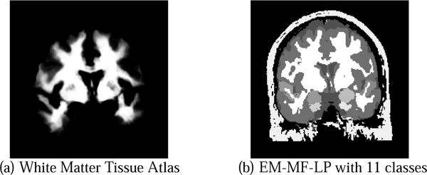
Segmenting brain with 11 tissue classes including left and right amygdala, superior temporal gyrus and parrahippocampal gyrus
4 Validation
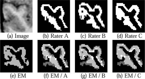
To validate this new approach, the left and right STG of four subjects were manually segmented by three raters. We used the Dice Similarity Measure (DSC) described by Zijdenbos et al. [16] to compare manual and EM-MF-LP segmentations. The is derived from the kappa statistic, where A1 and A2 are the two segmented areas. DSC > 70% is regarded as an excellent agreement between the two. In our approach, in all cases the similarity measure for the automatic segmentation was within the variance of the manual ones or above 70% (see Table 1(a)), which can also be observed in Figure 5.
Table 1.
Comparing the average DSC for one case and Warfield/Zou/Wells Measure between Rater A, B, C and the EM-MF-LP algorithm. The fraction in Table (b) is defined as . - means value was not available.
| (a) DSC Measure for one case | ||||||||
|---|---|---|---|---|---|---|---|---|
| Rater | A | B | C | EM | ||||
| A | 1.0 | 0.828 | 0.742 | 0.778 | ||||
| B | 0.828 | 1.0 | 0.744 | 0.825 | ||||
| C | 0.742 | 0.744 | 1.0 | 0.715 | ||||
| EM | 0.778 | 0.825 | 0.715 | 1.0 | ||||
| (b)Warfield/Zou/Wells Measure | ||||||||
| Rater\Case | 1 | 2 | 3 | 4 | ||||
| A |
|
|
|
|
||||
| B |
|
|
|
|
||||
| C |
|
|
|
|
||||
| EM |
|
|
|
|
||||
Fig. 5.
Comparing manual and automatic (EM-MF-LP) segmentation of the right STG where dark gray is EM-MF-LP only, light gray overlapping of manual and automatic, and white manual only segmentation.
The results were also compared with the performance measure introduced by Warfield et al. [17] (see Table 1(b)). This measure combines a maximum likelihood estimate of the ’ground truth’ segmentation from all the segmentations, and a simultaneous measure of the quality of each expert. The quality measure is composed of a sensitivity and specificity measures. A value of 1.0 for both is seen as perfect. Again, in all cases the automatic segmentation does as well as the manual ones. However, unlike manual segmentations, the algorithm can occasionally spread out over the ends of the STG into the middle temporal gyrus. In this segmentation the STG’s local priors do not compete with other neighbouring cortical substructures. Adding additional local tissue classes, like the middle temporal gyrus, would eliminate this effect and therefore further increase the accuracy of the automatic segmentation. Overall, the validation shows that the algorithm produces reliable results when compared with manual segmentations.
5 Discussion and Conclusion
In this paper we showed the benefits of integrating local tissue priors through non-rigid registration into the EM-MF. We validated the method by comparing it to manual segmentations of the STG. The results showed that the segmentation is comparable to manual ones. Through examples we showed that the algorithm performs better than some previous methods and is capable of more detailed segmentation including parcellation of the cortical structures. It also runs rapidly and robustly enough for further use in the real medical environment.
We believe the accuracy of the algorithm could be further increased by re-aligning the PPMs with the subject, by using the results of the segmentation and then re-segmenting the images again. When segmenting smaller structures, small errors can have large effects on the topology of the object, e.g. a voxel is assigned to a wrong class causing a structure to be separated. This effect could be limited by using higher order spatial information.
We believe that this approach is a step towards fully automated medical image processing, enabling the automatic segmentation of cortical sub-structures.
Fig. 4.
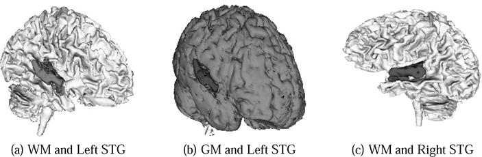
These figures show high quality, volumetric brain segmentations higlighting left and right STG
Acknowledgments
This investigation was supported by NIH grants P41 RR13218, P01 CA67165,R01 RR11747, R01 CA86879, by a research grant from the Whitaker Foundation, and by a New Concept Award from the Center for Integration of Medicine and Innovative Technology. We would especially like to thank for the helpful discussions with Dave Gering, Lauren O’Donnell and Samson Timoner.
References
- 1.Osher S, Sethian JA. Fonts propagating wiht curvature-dependent speed: Algorithms based on hamilton-jacobi formulations. J Comp Physics. 1988;79:12–49. [Google Scholar]
- 2.Leventon ME. Statistical Models in Medical Image Analysis PhD thesis, Massachusetts Institute of Technology. 2000 [Google Scholar]
- 3.Tsai A, Yezzi A, Wells W, III, Tempany C, Tucker D, Fan A, Grimson W, Willsky A. Model-based curve evolution technique for image segmentation. IEEE Conference on Computer Vision and Pattern Recognition. 2001 [Google Scholar]
- 4.Baillard C, Hellier P, Barillot C. Segmentation of 3d brain structures using level sets. Rapport interne IRISA. 2000;1291 [Google Scholar]
- 5.Fischl B, Salat DH, Busa E, Albert M, Dieterich M, Haselgrove C, van der Kouwe A, Killiany R, Kennedy D, Klaveness S, Montillo A, Makris N, Rosen B, Dale AM. Whole brain segmentation: Automated labeling of neuroanatomical structures in the human brain. Neuron. 2002;33 doi: 10.1016/s0896-6273(02)00569-x. [DOI] [PubMed] [Google Scholar]
- 6.Collins DL, Zijdenbos AP, Barre WFC, Evans AC. Animal+insect: Inproved cortical structure segmentation. Proc of the Annual Symposium on Information Processing in Medical Imaging. 1999;1613 [Google Scholar]
- 7.Warfield SK, Rexilius J, Kaus M, Jolesz FA, Kikinis R. Adaptive, template moderated, spatial varying statistical classification. Med Image Analysis. 2000;4(1):43–55. doi: 10.1016/s1361-8415(00)00003-7. [DOI] [PubMed] [Google Scholar]
- 8.Wells WM, III, Grimson WEL, Kikinis R, Jolesz FA. Adaptive segmentation of MRI data. IEEE Transactions on Medical Imaging. 15:429–442. 1996. doi: 10.1109/42.511747. [DOI] [PubMed] [Google Scholar]
- 9.Kapur T. Model based three dimensional Medical Imaging Segmentation PhD thesis, Massachusetts Institute of Technology. 1999 [Google Scholar]
- 10.Van Leemput K, Maes F, Vanermeulen D, Suetens P. Automated model-based bias field correction of MR images of the brain. IEEE Transactions on Medical Imaging. 1999;18(10):885–895. doi: 10.1109/42.811268. [DOI] [PubMed] [Google Scholar]
- 11.Warfield SK, Rexilius J, Huppi PS, Inder TE, Miller EG, Wells WM, Zientara GP, Jolesz FA, Kikinis R. A binary entropy measure to assess nonrigid registration algorithm. MICCAI. 2001 Oct;:266–274. [Google Scholar]
- 12.Thirion J-P. Image matching as a diffusion process: an analogy with Maxwell’s demons. Medical Image Analysis. 1998;2(3):243–260. doi: 10.1016/s1361-8415(98)80022-4. [DOI] [PubMed] [Google Scholar]
- 13.Guimond A, Roche A, Ayache N, Meunier J. Three-dimensional multimodal brain warping using the demons algorithm and adaptive intensity corrections. IEEE Transactions in Medical Imaging. 2001 Jan;20:58–69. doi: 10.1109/42.906425. [DOI] [PubMed] [Google Scholar]
- 14.Gering D, Nabavi A, Kikinis R, Hata N, O’Donnell L, Grimson E, Jolesz F, Black P, Wells W. An integrated visualization system for surgical planning and guidance using image fusion and an open MR. J Magn Reson Imaging. 2001;13:967–975. doi: 10.1002/jmri.1139. [DOI] [PubMed] [Google Scholar]
- 15.Pachai C, Zhu YM, Guttmann CRG, Kikinis R, Jolesz FA, Gimenez G, Froment J-C, Confavreux C, Warfield SK. Unsupervised and adaptive segmentation of multispectral 3d magnetic resonance images of human brain: a generic approach. 2001:1067–1074. [Google Scholar]
- 16.Zijdenbos AP, Dawant BM, Margolin RA, Palmer AC. Morphometric analysis of white matter lesions in MR images: Method and validation. IEEE Transactions on Medical Imaging. 1994;13(4):716–724. doi: 10.1109/42.363096. [DOI] [PubMed] [Google Scholar]
- 17.Warfield SK, Zou KH, Wells WM. Validation of image segmentation and expert quality with an expectation-maximazation algorithm,” in. MICCAI. 2002 [Google Scholar]