Statistical thinking for 21st century scientists

We offer a brief review of important questions concerning modern inference and how these questions relate to classical statistics.

Abstract

Statistical science provides a wide range of concepts and methods for studying situations subject to unexplained variability. Such considerations enter fields ranging from particle physics and astrophysics to genetics, sociology and economics, and beyond; to associated areas of application such as engineering, agriculture, and medicine, in particular in clinical trials. Successful application hinges on absorption of statistical thinking into the subject matter and, hence, depends strongly on the field in question and on the individual investigators. It is the job of theoretical statisticians both to be alive to the challenges of specific applications and, at the same time, to develop methods and concepts that, with good fortune, will be broadly applicable.

To illustrate the breadth of statistical concepts, it is helpful to think of the following sequence, in practice is often encountered in a different order:

1. Clarification of research questions in a complex situation.

2. Specification of the context for study, for example, the choice of individuals for entry into a clinical trial.

3. Issues of metrology: How are key features best measured in the context in question, and how secure is the measurement process?

Considered broadly, there may be many aspects of study design. The general aims are to achieve a reasonable level of precision, an absence of systematic error, and economy and breadth of interpretation, sometimes by answering several interconnected questions in one study. (i) Data collection, possibly including monitoring of data quality; (ii) data analysis, usually in various stages from the simple descriptive onward; (iii) summary of conclusions; (iv) interpretation:What is the underlying interpretation of what has been found? What are the relations with other work in the field? What new questions have been raised?

General statistical considerations may enter at all these stages, even though in essence they are all key subject matter concerns.

Phrases often heard nowadays are big data, machine learning, data science, and, most recently, deep learning. Big data have been around a long time, but the ability to analyze such data other than on a sampling basis is new. Key issues concern first the relevance of the data, especially if they are collected in a sense fortuitously. Then, there may or should be worries over quality. Some big data, for example, those obtained in the investigation at CERN leading to the Higgs boson, are of very high quality. However, in other situations, if a small amount of bad data may be quite misleading, a large amount of bad data may be exceedingly misleading. The third aspect is more technically statistical. The simpler methods of precision assessment may appear to indicate a very narrow confidence band on the conclusions from the big data, and this narrowness may give a seriously overoptimistic view of the precision achieved.

The other newer themes of statistical concepts involve important ideas coming with heavy computer science emphasis. These are often aimed at empirical prediction from noisy data rather than with probing the underlying interpretation of the data or with issues of study design or with the nature of the measurement process.

The theory and practice of computer-age statistics are, for the most part, a case of new wine in old bottles: The fundamental tenets of good statistical thinking have not changed, but their implementation has. This has been a matter of necessity. Data collection for a modern scientist can move in seven-league boots, thanks to spectacular advancements in equipment—notable examples include microarrays and DNA sequencers in microbiology and robotic telemetry for astronomy. Along with big data comes big questions; often, thousands of hypothesis testing and estimation problems are posed simultaneously, demanding careful statistical discussion.

Statisticians have responded with much more flexible and capacious analysis methods. These depend, of course, not only on the might of modern computation but also on powerful extensions of classical theories, which shift the burden of mathematical analysis onto computable algorithms but demand careful discussion for the formulation of principles. The examples that follow are too small to qualify as big data but, hopefully, are big enough to get the idea across.

A study at a pediatric hospital in Guatemala followed some 1800 children over a 12-year period beginning in 2002 (1). Ten percent of the children were abandoned by their families during their stay. The goal of the study was to identify the causes of abandonment. The key response variable was time, the number of days from admission to abandonment. For 90% of the children, abandonment was never observed, because of they left the hospital or the study period ended, in which case time was known only to exceed the number of days of observation. In common terminology, time was heavily censored.

More than 40 possible explanatory factors were measured, only 6 of which will be discussed here: distance, the distance of the child’s home from the hospital; date, the date of the child’s admission measured in days since the study’s beginning; age and sex of the child; and ALL or AML, indicating that the child was suffering from acute lymphoblastic leukemia (ALL) or acute myeloid leukemia (AML) (a worse prognosis). All of the variables were standardized. (Note that ALL and AML are two of several diagnoses under consideration, all of which were considered “others” for this analysis.)

Proportional hazards is a modern regression methodology that allows the fair comparison of potentially causative factors for a censored response variable (2). Table 1 shows its output for the abandonment study. Date for instance has a very strongly negative estimate, indicating that abandonment was decreasing as calendar time went on. Distance was strongly positive, suggesting increased abandonment from remote home locations. Neither age nor sex yielded significant P values, although there is some suggestion that older children did better. Likewise, neither ALL nor AML achieved significance, but, perhaps surprisingly, AML children seemed better off.

Table 1. Proportional hazards analysis of the abandonment data.

Estimated date coefficient of 1.660 is strongly negative, indicating decreased abandonment as study progressed.

	Estimate	SE	Z value	P value	Bootstrap
					SE
Distance	0.210	0.072	2.902	0.004	0.068
Date	–1.660	0.107	–15.508	0.000	0.088
Age	–0.154	0.084	–1.834	0.067	0.082
Sex	–0.027	0.076	–0.347	0.729	0.078
ALL	0.146	0.082	1.771	0.077	0.083
AML	–0.070	0.081	–0.864	0.387	0.088

In addition to the parameter estimates (Table 1, column 1), proportional hazards theory also provides approximate standard errors (column 2). The bootstrap (3) was used as a check. Each bootstrap data set was formed by sampling the 1800 children 1800 times with replacement; thus, child 1 might appear twice, child 2 not at all, child 3 once, etc. Then, the proportional hazards model was run for the bootstrap data set, giving new estimates for distance, date, age, sex, ALL, and AML. Two thousand bootstrap data sets were independently generated, yielding the bootstrap standard errors in column 5 of the table. For instance, the 2000 bootstrap estimates for distance had an empirical SD of 0.068, nearly the same as the theoretical SE of 0.072. With the moderate exception of date, the other comparisons were similarly reassuring.

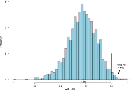
The bootstrap replications can be used to address a variety of other inferential questions. Figure 1 shows the histogram of the 2000 bootstrap estimates of the difference AML minus ALL. Only 34 of the 2000 exceed 0, yielding a one-sided bootstrap P value of 0.017 (34 of 2000) against the null hypothesis of no difference.

Fig. 1. Two thousand bootstrap replications of difference between AML and ALL proportional hazards coefficients.

The proportional hazards algorithm required perhaps 100 times as much computation as a standard linear regression, whereas the bootstrap analysis multiplied the burden by 2000. Neither theory would have been formulated in the age of mechanical calculation. They are discussed in chapters 9 and 10 in the study of Efron and Hastie (4), along with a suite of other computer-intensive statistical inference methods.

At the fundamental level, statistical theory concerns learning from experience, especially from experience that arrives a little bit at a time, perhaps in noisy and partly contradictory forms. Modern equipment allows modern scientists to cast wider experiential nets. This has increased the burden on the statistical learning portion of the scientific process. Our next example, taken from chapter 6 in the study by Bradley and Hastie (4), shows the learning process in action, using statistical ideas proposed in the 1950s but which are only now routinely feasible.

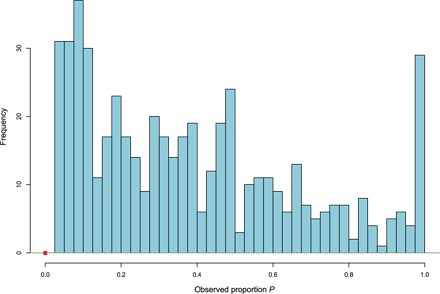
Figure 2 concerns a study of 844 patients undergoing surgery for stomach cancer. Besides the removal of the central site, surgeons often remove surrounding lymph nodes, malignant or negative. For patient i, i = 1, 2, …, 844, let

$$\begin{array}{c}{\mathit{n}}_{\mathit{i}}=\# \text{nodes removed}\\ {\mathit{x}}_{\mathit{i}}=\# \text{nodes positive}\end{array}$$

and

$${\mathit{p}}_{\mathit{i}}={\mathit{x}}_{\mathit{i}}/{\mathit{n}}_{\mathit{i}}$$

where p_i is the proportion of positive nodes; n_i varied between 1 and 69. The histogram in Fig. 2 depicts the 522 patients with p_i > 0, that is, having at least one positive node; 322 of the patients, about 38%, had p_i = 0, represented by the large dot.

Fig. 2. Observed proportion P of malignant nodes for 522 patients having P > 0; 322 patients (38%) had P = 0, as indicated by the large dot.

It is reasonable to imagine that each patient has a frailty parameter θ_i, indicating how prone he or she is to positive nodes and that we are seeing binomial observations

$${\mathit{x}}_{\mathit{i}}~ \text{binomial}({\mathit{n}}_{\mathit{i}},{\mathrm{\theta }}_{\mathit{i}})$$

Equivalently, x_i is the number of heads observed in n_i independent flips of a coin having a probability of heads θ_i. If the n_i’s were large, then p_i = x_i/n_i would nearly equal θ_i. However, many of the n_i’s were small (eight of them equaling 1); hence, Fig. 2 gives a badly distorted picture of the distribution of the θ_i’s.

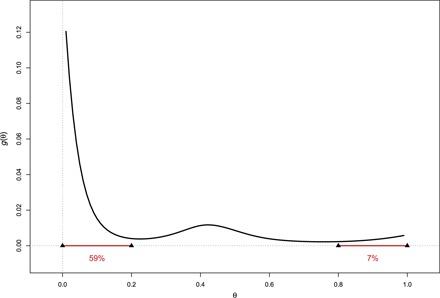
Empirical Bayes methods allow us to recover a good estimate of what a histogram of the 844 true θ_i values would look like. We assume that the θ_i’s have some prior density g(θ); g(θ) is unknown but assumed to belong to a low-dimensional parametric family. Here, log g(θ) was assumed to be a fifth-order polynomial in θ. Maximizing the likelihood of the observed data (n_i, x_i), i = 1, 2, …, 844, over the coefficients of the polynomial yielded the estimate of g(θ) pictured in Fig. 3. It shows that most of the frailties are small (59% less than 0.2), but there are large ones too (7% above 0.8).

Fig. 3. Estimated prior density for frailty parameter θ, with median value θ = 0.09.

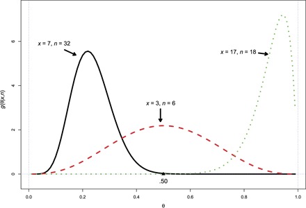
Having estimated the prior density g(θ), we can use the Bayes rule to calculate the posterior density of θ_i given patient i’s observed values n_i and x_i. This is done for three of the patients in Fig. 4. Patient 1, with n_i = 32 and x_i = 7, is seen to almost certainly have θ_i less than 0.5; patient 3, with n_i = 18 and x_i = 17, almost certainly has frailty θ_i greater than 0.5; and patient 2, with n_i = 6 and x_i = 3, could conceivably have almost any value of θ_i. This kind of information may be valuable for recommending follow-up therapy that is either more stringent or less.

Fig. 4. Posterior probabilities of frailty parameter θ for three hypothetical patients.

The observed data n_i = 32 and x_i = 7 represent direct statistical evidence for patient 1. It provides, among other things, the direct estimate P₁ = 7/32 = 0.22 for θ₁. Indirect evidence, from the other 843 patients, also contributed to the posterior probability density for patient 1 depicted in Fig. 4.

An increased acceptance of indirect evidence is a hallmark of modern statistical practice. Both frequentist techniques (regression algorithms) and Bayesian methods are combined in an effort to bring enormous amounts of possibly relevant “other” cases to bear on a single case of particular interest, that is, patient 1 in the nodes study. Avoiding the difficulties and pitfalls of indirect evidence motivates much of current statistical research.

We emphasize the current high level of fruitful application and methodological development. However, this is anchored in a long history going back particularly to the great early 19th century mathematicians, Gauss and Laplace. Their statistical work was motivated by concerns over the analysis of astronomical data. Quasi-philosophical disagreements over the meaning of probability have rumbled on since then. Our attitude is eclectic, but in the last analysis, we see a contrast, not a conflict, between the use of probability to represent in idealized form patterns of variability in the real world and its use to capture the uncertainty of our conclusions. Controversy centers mostly on the second, and more than one approach may be fruitful. However, in the last analysis, we are using probability as a measuring instrument, and in some sense, it must be well calibrated.

We have worked as statisticians for a combined total of 125 years (72 and 53 years of experience, respectively) and both of us fully retain our enthusiasm for the field. It has changed enormously over our lifetimes and no doubt will continue to do so. Yet, at the heart of our subject are core issues about uncertainty and variability that have both a permanent value and an exciting continuing challenge that is conceptual, mathematical, and computational.

SPECIAL NOTE: The Editors invited authors David Cox and Bradley Efron to submit this article to honor their receipt of the 9th Edition (2016) BBVA Foundation Frontiers of Knowledge Award in Basic Sciences for revolutionizing statistics.

References

- 1.E. Alvarez, M. Seppa, K. Messacar, J. Kurap, E. A. Sweet-Cordero, S. Rivas, M. Bustamante, L. Fuentes, F. Antillón-Klussmann, P. Valverde, M. Castellanos, S. C. Howard, B. Efron, S. Luna-Fineman, Improvement of abandonment of therapy in pediatric patients with cancer in Guatemala. J. Glob. Oncol. 10.1200/JGO.2016.004648 (2016). [DOI] [PubMed] [Google Scholar]
- 2.Cox D. R., Regression models and life-tables. J. Roy. Stat. Soc. B 34, 187–220 (1972). [Google Scholar]
- 3.Efron B., Bootstrap methods: Another look at the jackknife. Ann. Stat. 70, 1–26 (1979). [Google Scholar]
- 4.B. Efron, T. Hastie, Computer Age Statistical Inference: Algorithms, Evidence, and Data Science (Cambridge Univ. Press, 2016). [Google Scholar]