Squeezing of Ion Populations and Peaks in Traveling Wave Ion Mobility Separations and Structures for Lossless Ion Manipulations Using Compression Ratio Ion Mobility Programming

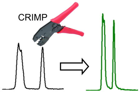
Abstract

In this work we report an approach for spatial and temporal gas-phase ion population manipulation, wherein we collapse ion distributions in ion mobility (IM) separations into tighter packets providing higher sensitivity measurements in conjunction with mass spectrometry (MS). We do this for ions moving from a conventional traveling wave (TW)-driven region to a region where the TW is intermittently halted or “stuttered”. This approach causes the ion packets spanning a number of TW-created traveling traps (TT) to be redistributed into fewer TT, resulting in spatial compression. The degree of spatial compression is controllable and determined by the ratio of stationary time of the TW in the second region to its moving time. This compression ratio ion mobility programming (CRIMP) approach has been implemented using “structures for lossless ion manipulations” (SLIM) in conjunction with MS. CRIMP with the SLIM-MS platform is shown to provide increased peak intensities, reduced peak widths, and improved signal-to-noise (S/N) ratios with MS detection. CRIMP also provides a foundation for extremely long path length and multipass IM separations in SLIM providing greatly enhanced IM resolution by reducing the detrimental effects of diffusional peak broadening and increasing peak widths.

Graphical abstract

Mobility-based gas-phase ion separations, including drift tube ion mobility (DTIM),^1–3 field asymmetric ion mobility spectrometry (FAIMS),⁴ differential mobility,^5,6 overtone mobility,⁷ trapped ion mobility spectrometry (TIMS),^8,9 and traveling wave ion mobility (TWIM),^10,11 are of increasing analytical utility for distinguishing charged species not feasible by mass spectrometry (MS) alone. Each separation has been utilized for different applications to provide capabilities not possible with other separation techniques.

In TWIM separations, higher mobility ions tend to move with the TW while lower mobility ions are more frequently passed over by waves, resulting in mobility-dependent separation for all charged species below a mobility threshold. ^12–15 TWIM separations use a repeating and moving voltage profile to drive ion mobility separations.¹⁰ If DTIM were used, exceedingly high voltages would be necessary to move ions through very long paths. However, TWIM operates with a low revolving voltage, making long path lengths possible. TWIM is particularly attractive in conjunction with structures for lossless ion manipulations (SLIM)^12,13 where we can fashion extended ion separation paths, as well as construct switches, reaction regions, and traps from electric fields using combinations of rf and dc potentials applied to appropriate electrode arrays on two planar and closely spaced surfaces.^13–15 SLIM provide the basis for complex and otherwise impractical combinations of ion manipulations over extended times.¹⁶ Of particular relevance here are the recent demonstrations using extended serpentine paths in SLIM for achieving greatly increased IM resolution.^16–18

While SLIM now arguably provide a basis for ultrahigh IM resolution in conjunction with high sensitivity,^16–18 long path length separations can give rise to exceedingly large peak widths due to diffusion and other factors. We have observed that TWIM separations (using our SLIM platform) provide higher resolution than DTIM for a given path length, but also entail greater peak broadening.¹³ Regardless of its origin, peak broadening in IM separations results in lower signal intensities and reduced signal-to-noise (S/N) ratios as path lengths increase, limiting the maximum useful path length. This limitation due to diffusion is particularly evident for multipass designs where ions execute more than one passage through the ion path.¹⁷ In addition, multipass designs also entail a progressive reduction in the range of ion mobilities effectively examined with each pass to avoid the “lapping” of peaks and are also ultimately limited by the expansion of the peak (or peaks) of interest across the entire separation path. The ability to reduce the peak widths in a multipass separation would enable addressing these issues.

We have recently discussed the utility of IM peak spatial compression in the context of DTIM separations.¹⁹ The DTIM approach, however, was limited by practical electric field constraints in the extent of compression achievable as well as the range of mobilities to which it could be applied.¹⁹ Here we report a new and broadly applicable approach for IM peak compression based upon the use of traveling waves. In TW-based IM separations the ions in a peak will typically be dispersed across some number of “traveling traps” (TT), which are the periodically occurring potential minima of the TW troughs. In the compression approach we report, ions spanning a number of TT in a first conventionally TW-driven region move through an interface to a second region having intermittently moving TW (i.e., stuttering traps; ST). Thus, ions effectively redistribute into a smaller zone (i.e., fewer TT “bins”) at the TT/ST interface, and ion populations (partial or full IM separations) are compressed in a controllable fashion by an arbitrary integer value, which is defined as the compression ratio (CR). This spatial compression step is followed by programmed switching of the ST region to a nonstuttering TT mode. This can be done to resume separation if desired, typically using the initial TT conditions, albeit with narrower IM peaks than prior to compression.

The present work describes both the theoretical considerations related to compression ratio ion mobility programming (CRIMP) and its initial experimental implementations using SLIM. The reported developments are of general utility for the spatial manipulation of ion populations, and more specifically address the major challenges of using extended path SLIM designs for achieving much greater IM resolution while simultaneously maintaining the signal intensities and sensitivity.

EXPERIMENTAL SECTION

Ion motion simulations were performed using SIMION 8.1 (Scientific Instruments Services (SIS) Inc., New Jersey, U.S.A.). The SDS collision model was used to model the ion motion in 4 Torr N₂.^13,14 The simulated geometries were based upon SLIM printed circuit board (PCB) components developed for experimental studies and were generated using EagleCAD software (CAD Soft Inc., Germany). The TW voltages were defined using a “Lua” code and interfaced with SIMION 8.1. Experimentally, ions were introduced from a nanoelectrospray ionization (nanoESI) source into the first stage of vacuum housing an ion funnel trap (IFT)² (2.45 Torr, 820 kHz, 200 V_p-p), followed by a SLIM module at (~2.50 Torr), as shown in

Figure 1a. This module has interleaved rf and dc electrodes (Figure 1a) similar to that previously described.¹⁶ Ions were introduced from the IFT either continuously or “pulsed” as ion packets (of <0.5 ms width) after a period of accumulation. The IM paths are created using electric fields resulting from rf and dc potentials applied to arrays of electrodes,¹⁶ and previously demonstrated to effectively confine ions, allowing their transport and IM separations using TW. Ions exit the SLIM module to a “rear” ion funnel (2.50 Torr, 750 kHz, 120 V_p-p) and were transmitted through a short quadrupole (170 mTorr, 960 kHz, 340 V_p-p) to an Agilent 6538 QTOF MS (Agilent Technologies, Santa Clara, CA). Data were recorded using a U1084A 8-bit ADC digitizer (Keysight Technologies, Santa Rosa, CA) and processed using in-house software. Ion currents transmitted through the SLIM were measured in some experiments using a fast current inverting amplifier (model 428, Keithley Instrument Inc., Cleveland, OH) and a TDS-784C digital oscilloscope (Tektronix, Richardson, TX).

Figure 1.

(a) Schematic of the experimental arrangement. The SLIM electric fields were generated by potentials applied to two parallel surfaces with electrodes arranged as described in the text, to create a 13 m long IM separation path. The inset on the right shows a detailed view of a small portion (at a turn) of the electrode arrangement on one of the two SLIM surfaces, and the left inset shows a small portion of two parallel surfaces of the SLIM corresponding to the length of one eight-electrode repeating unit. (b) Left panel shows the contours lines of the rf effective potentials in the XY plane (i.e., plane normal to the axial direction of ion motion). Center panel shows isopotential surface (at 100 V) showing the confinement region forming ion “conduits” or ion “pipes” Ions are confined to a conduit defined by the central oval region between the two surfaces. The right panel shows the TW potential distribution in the XZ plane for a 80 TW electrode segment (or ~8 cm of the path) between the two SLIM surfaces and where ions are confined in the TT mode (see text) by the potential minima.

The SLIM module used in this work was a nominal 13 m serpentine multipass design (to be described in detail in a future manuscript).²⁰ The SLIM designs used a pair of evenly spaced surfaces (~3 mm gap) having mirror-image arrays of six rf strip electrodes and lateral ion-confining dc “guard” electrodes, as described previously.^13,16 Five strips of segmented TW electrodes of 1.03 mm length and 0.43 mm width were interspersed between adjacent oppositely phased rf electrodes (a small portion of one surface is shown in the inset of Figure 1a). The segmented TW electrodes were supplied with a voltage profile that was repeated for each set of eight adjacent electrodes to create the TT or ST that propel ions through a serpentine 13 m multipass SLIM module. Ion packets were manipulated by programmatically adjusting the voltages applied to the TW electrodes as described in this work.

RESULTS AND DISCUSSION

We report a highly flexible approach for spatially compressing ion populations by a predetermined compression ratio (CR) and specifically describe it in the context of IM separations with a present focus on enabling more effective and much higher resolution separations. We refer to this overall process as “compression ratio ion mobility programming” (CRIMP). In this work the ion spatial compression occurs in devices having two different regions, the first operating in a conventional TT mode, and a second ST region that can be halted periodically to achieve compression for specified times during extended manipulations (as in multipass separations). The key compression step occurs at the interface between the two regions where the ST in the second region presents a trapping region for the accumulation of ions spread over multiple TTs as the ions approach the TT/ST interface from the first region. Once this spatial compression is accomplished, the ST region is switched back into the normal TT mode to retain the compression in the temporal domain. The application of this compression step depends on the careful control of timing for the resumption of conventional TT conditions in the second region after the desired spatial compression event is completed. We note that, once the spatial compression process is accomplished, this switching from ST mode to the TT modes must be performed while the spatially compressed ion distribution (e.g., multiple IM peaks) is still within the ST. If an ion distribution is still in the ST mode (with intermittently moving traps) when it moves into a conventional TT region all the benefits of the spatial compression will be lost as the packets will be “decompressed” at this ST/TT interface. It is important to emphasize that CRIMP can involve multiple compression events during the course of multipass IM separations to both control the growth of peak widths and the range of mobilities that can be studied. Such IM separations can avoid limitations on the range of mobilities effectively studied (by avoiding lower mobility species being lapped by higher mobility species) and can also benefit from compression applied prior to detection to enhance peak intensities and sensitivity.

Our initial implementation of CRIMP benefitted from the flexibility and relative ease of fabrication afforded using SLIM and has specifically aimed to address key challenges of multipass IM separations for providing greatly enhanced resolution. In this work the TW potentials applied to the TT and ST regions were coordinated, but were separately controlled to provide the intermittent STs used part of the time in the second region. The TW potentials (50 V maximum) were applied to each four adjacent electrodes of each eight-electrode array extending along the ion path (i.e., across many eight electrode sets), with the applied profile moving by stepping in single electrode steps with a frequency dependent on the desired TT speed. For example, in the 00001111 sequence, “0” represents the low voltage used and “1” represents the high voltage used.¹³ Figure 1b (left) shows an image of the confining field between the electrode surfaces in the “XY” plane (the plane normal to the axis of ion motion). Figure 1b (center) shows a 3-D representation of an isopotential (at 100 V) surface created by SLIM rf and TW electrode potentials. The enclosed region is the confining surface that retains ions within ion “conduits” and transports them along the direction of the TW motion. Figure 1b (right) shows the TW potentials along the ion motion path in the XZ plane (equidistant from each surface, with one of the surfaces displayed), spanning 80 TW electrodes along the IM path and used to create the TW (both TT and ST). Ten TT created by the applied TW and guard voltages are evident. The ions thus remain confined within the SLIM ion conduits and are driven by the applied TW profiles. If the TW is sufficiently slow or stationary, the ions remain confined within the TT (i.e., the TW troughs shown in Figure 1b, right). When the TT speed is sufficiently high, and depending on the mobility, ions can be periodically passed over by a TW, i.e., rollover into the preceding TT. Thus, for a TT speed greater than some threshold, ions have a mobility-dependent probability of being passed over by a wave, leading to separation. In this process peaks broaden due to both diffusion and also an extra diffusion TW-related component. Thus, an IM peak will span an increasing number of TT as a separation progresses.

In CRIMP, ions that are moving (either confined to traveling traps or in the separation mode and occupying some number of TT) in the first region transition to a second region where they are redistributed into a smaller number of ST. Figure 2a gives a schematic of the CRIMP process for CR = 2. In step 1 ions distributed over multiple TT, with each TT packet represented by a colored oval in Figure 2a, and where the red electrodes have an elevated voltage forming the TT that moves to the right. In step 2 the TT enters the second region (i.e., the TT/ST interface) during a period when it is stationary, causing a merging of the TT contents with any other ions already residing in the ST, and leading to spatial compression. We note that an alternative approach for this step 2 would involve the transition to a second region with the traps having a smaller size due to the use of shorter TW segmented electrodes, or alternatively with the use of a different TW sequence (e.g., 00110011 rather than 00001111). However, these alternative approaches would only allow CRs corresponding to the ratio of electrode lengths in the two regions, or by a factor of 2 for the indicated sequence change. In principle CRIMP allows CR of any integer value as it depends only on the time the TW is paused in the ST region. In practice, the CR should be applied with consideration of the initial peak widths. For example, assuming that a minimum of 5 TT need to be sampled to accurately define a Gaussian peak, then the initial peak should span at least ~5 × CR TT. In addition, constraints provided by space charge limit the maximum compressibility of the ion packet. Step 3 involves the resumption of wave motion in the ST region, and step 4 represents the initial halting of the TW and the return to step 1 for compressing the next set of incoming TTs. After a number of such compression steps (repeated to cover some portion, or all, of the separation), the selected region (or mobility range) from the first TT region will be spatially compressed in the second ST region. Subsequent to this spatial compression, and before ions exit the second region, there is a transition from ST operation to the TT mode in the second region, to “lock in” the compression and effectively provide temporal compression. In principle, CRIMP can be used to compress any IM separation or other ion distribution to an arbitrary degree. In practice, the finite size and charge capacity of each TT makes the use of CRIMP much more effective for broad low-abundance peaks than for narrow high-abundance peaks.

Figure 2.

(a) Schematic representing the CRIMP process. (b) Simulation showing lossless ion transport in the SLIM device during CRIMP. (c) Simulation showing spatial peak compression at the TT/ST interface.

To initially evaluate CRIMP, ion trajectory simulations were performed using SIMION 8.1. A TW speed of 50 m/s was used in the TT region and indicated lossless performance throughout. Figure 2b show the ion trajectories through the device in the XZ plane (top panel) and in the YZ plane between the surfaces (bottom panel). Simulations were performed with four electrodes at 50 V, four electrodes at 0 V, and at 50 m/s TT speed. The ST region was operated with the same voltage configuration as the TT region, but with a duty cycle of 33% (i.e., combining three TT bins into 1 ST; CR = 3). Since ions surf under the selected conditions, those occupying a single TT (each four electrodes wide) are expected to remain confined to the TT through the point of merging into the ST. In the simulations ions distributed uniformly over three adjacent TT (Figure 2c, black lines) merge into one ST at the TT/ST interface, providing a reduction in peak width and an increase in peak height (Figure 2c, blue line). Subsequent to this spatial compression, normal TW conditions are imposed in second region before the compressed zone of the separation exits the second region.

Our experimental validation of this approach used a 13 m multipass SLIM module divided into two regions with independent TWs applied to each. While the synchronization of the TW in both regions was retained, the switching of TW potentials was intermittently halted in the ST region to provide the desired CR. The first SLIM region was 9 m in length, and the second region was 4.5 m in length (see Figure 3a). The length 4.5 m for the second region allowed a distribution spanning the whole of the first region (9 m) to be compressed for CR = 2 and above (and also time for subsequent switching to normal TT mode after compression). After the second region, ions exited the SLIM and entered the rear ion funnel (Figure 1a). A timing diagram for the TT and ST regions is shown in Figure 3b; the left panel shows the TT and ST frequency in these regions. While the TT conditions in the first region have a constant TW speed (i.e., a constant frequency of the wave motion), the motion of the TW in the ST region is intermittent during the chosen times when peak compression is executed, with normal TT conditions applied at all other times. The potential applied to the first electrode of the ST region as a function of time is shown in Figure 3b (right panel). When the second region is operated in the normal TT mode, the voltage changes at uniform intervals as the wave moves forward. However, in the ST stuttering/compression mode, the stationary period of the voltage profile is evident by the longer times for which the electrode remains at the same voltage (0 V in this case). The CR is determined by the ratio of stationary time versus moving time for the voltage profile in the ST region. For example, a stationary time (indicated by the time for which the frequency of the wave is zero in Figure 3b) for the ST that is twice the moving time causes two TT to be merged in the ST before it moves forward, thus providing a CR of 2. Larger stationary periods of the ST provide larger CR. The timing diagrams (as directly measured by the oscilloscope) for the second and fifth electrodes after the TT/ST interface are shown in Supporting Information Figure S1. Thus, the first four electrodes are at a lower potential while the next four electrodes are at a higher potential (i.e., a 00001111 sequence). This profile is applied for a longer period of time in the ST region as compared to profile in the TT region. This allows ions to be accumulated in the low-potential region (first four electrodes for each of four segmented strips) as they enter the TT/ST interface. The maximum CR is ultimately limited by the accumulation of excessively large ion populations and the resulting space charge effects. As noted previously, the useful CR is also constrained by the minimum number of bins needed to define the peak with a desired level of accuracy (which in the case of sampling a chromatographic peak is conventionally considered to be in the range of 5–10).²¹

Figure 3.

(a) Schematic showing the traveling trap (TT) and stuttering trap (ST) regions of the SLIM. (b) Timing diagram of the TW speed/frequency and electrode voltages for CRIMP are shown. In the left panel the TW frequency applied in the TT region and ST region is shown, with the ST region experiencing intermittent wave velocity represented by periodically stopping waves at 0 kHz frequency. The right panel shows the voltage of the first electrode in the TT/ST interface. When in the normal TT mode the amplitude varies between 50 and 0 V at equal intervals, while in the ST mode the voltage experiences 0 V for longer times corresponding to times when the wave is stationary.

Figure 4 shows ion current measurements (at the quadrupole after the exit ion funnel; Figure 1a) for a 100 ms wide ion pulse from the IFT, both without and with compression. This 100 ms pulse is spread over ~1000 bins (the width of each bin is approximately four electrodes or 4.1 mm, and each bin is spaced another 4.1 mm apart), with the TT speed of 82 m/s. The present work used “surfing” condition (i.e., where the ions moved with the TT and without rolling over) to perform CRIMP. Therefore, all ions regardless of mobility traveled at the same speed simplifying timing for these initial experiments using CRIMP. We emphasize that CRIMP can also be performed in the separation mode with knowledge of separation, which can be obtained from a prescan experiment of the analytes or from theoretical considerations. Thus, a peak spanning 100 ms (Figure 4, blue trace) is spread over a number of bins given by $N_{\text{bins}}=\frac{82\left[\frac{\mathrm{m}}{\mathrm{s}}\right]\times 100[\text{ms}]}{(4.1[\text{mm}]+4.1[\text{mm}])}=1000\text{TT}$, or ~8.2 m of the 9 m long first region (see Figure 3a); the ion population spans almost the entire region from the SLIM entrance to the TT/ST interface. When we apply CR = 10, every 10 TT of the original peak are combined into one ST. Subsequently, the ST region is switched back to the TT mode before ejection to the detector. Thus, after compression ions are expected to span ~100 bins (~0.82 m length of the ST region). Since the ST region has a length of 4.5 m, the band was fully contained within the ST region, and the subsequent change in the voltage profile to the TT mode is expected to result in compressed peak width of $10\text{ms}\left(\frac{100[\text{bins}]\times 8.2\left[\frac{\text{mm}}{\text{bin}}\right]}{82\left[\frac{\mathrm{m}}{\mathrm{s}}\right]}\right)$, consistent with experiment (Figure 4, green). This reduction in peak width is accompanied by a nearly 10-fold gain in peak height. The area under each peak was calculated and found to be preserved before and after compression (~25 million charges) within measurement uncertainty and consistent with essentially lossless performance.

Figure 4.

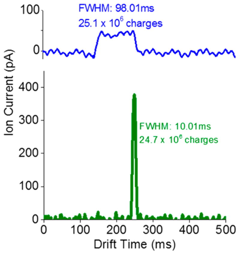
CR = 10 peak compression applied to a 100 ms wide packet introduced into the 13 m long path SLIM used in this work, showing effective and lossless peak width reduction.

Potential effects on IM peak width and resolution with CRIMP arise from the ion packet “quantization” (due to the finite TT size). Consider two peaks with mobilities of K₁ and K₂ moving with average speeds 〈v₁〉 and 〈v₂〉 in a TW separation, having undergone a separation for an initial time t₀. The time separation between the two peaks after t₀ can be estimated by the equation: $\mathrm{\Delta }T=\left(\frac{\langle {\nu }_1\rangle }{\langle {\nu }_2\rangle }-1\right)t_0$. We assume that subsequent to initial separation time (t₀), the peaks are subjected to CRIMP. For simplicity we assume that ions are in the surfing mode (i.e., move with the TT) during compression, and we note that a transition to this mode is potentially achievable by simply increasing the TW amplitude. The number of TT that span a separation between two peaks originally separated by ΔT can be given as

$$\mathrm{\Delta }{N}_{\text{bins}}=\lfloor \frac{s}{x_{\mathrm{w}}}\mathrm{\Delta }T\rfloor$$ (1)

Here “s” is the speed of the TW, “x_w” is the width of a single TT (e.g., the width of each TW trough as in Figure 1b, right panel), and the function ⌊x⌋ represents the floor function operated on variable “x” (i.e., ⌊x⌋ = the nearest integer value lesser than x). For such peak compression performed at a selected CR, the new separation between the two peaks will span a number of TT “ ΔN_compressed” with a temporal separation ΔT_compressed given by

$$\mathrm{\Delta }{N}_{\text{compressed}}=\lfloor \frac{1}{\text{CR}}\lfloor \frac{s}{x_{\mathrm{w}}}\mathrm{\Delta }T\rfloor \rfloor$$ (2)

$$\mathrm{\Delta }{T}_{\text{compressed}}=\frac{x_{\mathrm{w}}}{s}\lfloor \frac{1}{\text{CR}}\lfloor \frac{s}{x_{\mathrm{w}}}\mathrm{\Delta }T\rfloor \rfloor$$ (3)

The floor function by eqs 2 and 3 provides a lower estimate to the number of TT spanning a separation after compression, with the uncertainties related to the detailed parsing of the ion distribution into TT. Similarly, the peak full width at half-maximum (fwhm) after compression can be expressed in terms of the fwhm before compression (〈t_fwhm〉) as

$${\langle t_{\text{fwhm}}\rangle }_{\text{compressed}}=\frac{x_{\mathrm{w}}}{s}\lceil \frac{1}{\text{CR}}\lceil \frac{s}{x_{\mathrm{w}}}\langle t_{\text{fwhm}}\rangle \rceil \rceil$$ (4)

Here, ⌈x⌉ represents the ceiling function operated on a variable “x” (i.e., ⌈x⌉ = the nearest integer value greater than x). Thus, using eqs 3 and 4, a lower bound on the obtained resolution after compression is given by eq 5; eq 3 gives the lowest possible value of the time separation after compression, and eq 4 gives the highest value of the peak width that may be obtained after compression, assuming that the ions are distributed uniformly within any given bin.

$$R_{\text{compressed}}\ge \frac{\lfloor \frac{1}{\text{CR}}\lfloor \frac{s}{x_{\mathrm{w}}}\mathrm{\Delta }T\rfloor \rfloor }{\lceil \frac{1}{\text{CR}}\lceil \frac{s}{x_{\mathrm{w}}}\langle t_{\text{fwhm}}\rangle \rceil \rceil }$$ (5)

Theoretically any integer CR may be used until either space charge limit is reached or the final peaks widths are excessively narrow (covering <~5 TT).

CRIMP can greatly benefit long-path IM separations, where periodic application can offset diffusional peak broadening. To demonstrate this the 13 m SLIM module (shown in Figure 1a) was enabled with a multipass capability (to be described in detail in a future manuscript) allowing ions to either be switched to the MS or switched back to the original path to execute another pass. Using CRIMP with such a multipass device has many possible modes of application and provides a general basis for obtaining increased peak heights while maintaining peak resolutions (as indicated by eq 5). Figure 5a shows the peak widths, separations, and resolution predicted using eq 5 (for ions with mobilities corresponding to the isomers of lacto-N-hexaose; see below). The effect of peak compression on peak width, separation and resolution in an extended (long path) separation is evident. These calculations serve to emphasize two important points. First, the resolution achievable with CRIMP can only approach that achievable without CRIMP if there are no constraints related to IM path length and sensitivity for peak detection, e.g., the resolution achieved in a given time will always be less, but the difference can be negligible with proper application. Second, when real-world constraints on path length and detection exist CRIMP provides significant benefits, constraining the growth in peaks widths, the narrowing of the mobility range in multipass separations, and allowing greater resolution to be achieved. CRIMP application is most effective when the individual peak widths, i.e., their traveling trap or “bin counts”, are not excessively narrow after compression is applied. As shown in Figure 5a, after compression there is a decrease in both the separation between peaks and the width of peaks. Thus, application of excessive CR using CRIMP resulting in very narrow peaks after compression (e.g., less than approximately 5–10 traveling traps or bins at half-height) can lead to significant loss of resolution.

Figure 5.

(a) Left, theoretical prediction of the peak separation and peak widths without (black) and with (blue) multiple compression events; right, theoretical resolution without (black) and with (blue) peak compression. The inset shows the recovery time (i.e., added separation) needed is small for regaining the small loss of resolution from compression. Also, subsequent to recovery, the peak height remains significantly increased. (b) Experiment measurements showing resolution for the m/z 622 and 922 peaks for three situations: left, separation after two passes; center, separation after three passes; right, separation after two passes with CRIMP CR = 2 then applied, showing similar resolution as two passes but with increased peak heights.

For an initial demonstration of a simple application of CRIMP in a multipass separation we used a mixture of lacto-N-hexaose (LNH) and lacto-N-neohexaose (LNnH) and 0.48 ms packets of ions injected from the IFT, both with and without compression. The left panel of Figure 5b shows the separation after ~27 m (two cycles; left), and after ~40 m (three cycles; center), without compression. Using CRIMP with CR = 2 after two cycles of separation, the peak height was increased by ~1.6-fold. The spectrum on right panel of Figure 5b corresponds to same path length traversed as in Figure 5b, center panel, but with only two cycles of separation and the third pass constituting the “surfing” mode and peak compression. Thus, the separation obtained after two cycles (Figure 5b, left panel) is preserved in the surfing mode and after compression with only a modest loss in resolution (0.9 from Figure 5b, left before compression, 0.85 in Figure 5b, right after compression). This minor loss of peak resolution is easily recovered by additional separation following peak compression (as indicated by recovery time t_R = 10 ms; Figure 5a, right panel), at which point the peak width is still significantly lower than without compression (~1.8-fold thinner peaks and correspondingly higher S/N). In the present work we maintained surfing conditions after two cycles of separation (i.e., through the compression and until switching for ejection to the MS). We note our intent to implement more sophisticated programming of CRIMP to allow an arbitrary number of separation cycles followed by an arbitrary CR and resumption of separation cycles for arbitrary number of cycles prior to detection. This capability for precisely timing the application of CRIMP to target a mobility range window will allow improvement in S/N ratios over chosen mobility ranges, or of an entire separation. One significant advantage of TW-based CRIMP over previously reported peak compression approaches for drift field IMS¹⁹ (where a nonconstant electric field is applied periodically) is that the effects of compression are not mobility-dependent. As the ions remain effectively confined within traveling traps during CRIMP, a set compression ratio CR would enable all “real” ions to be rebinned into a smaller number of traveling traps without any bias. Also, as long as the spatially compressed peaks are returned to normal (i.e., nonstuttering) TW conditions by proper timing of this event (i.e., before exiting the ST region), the peak compression will be temporally preserved. In instances when only a portion of peak is within the ST region and some part of the peak has already exited the ST region before switching to normal TW, a reversal of the compression (i.e., decompression) would take place at the ST/TT interface, and the possibility of some loss of resolution. However, this is easily avoided by proper application of CRIMP.

To further demonstrate CRIMP, 25 ms wide bands of ions (significantly wider than the <0.5 ms pulses typical of IFT-based injection) were injected into the 13 m SLIM to emulate very broad peaks and also as the starting point for separations. The first 9 m TT region the SLIM was operated in a separation mode, and the second 4.5 m ST region was operated in the surfing mode. This preserved the separation achieved in the first 9 m, providing the separation shown in Figure 6a. Separation is obtained for the two species [m/z 622; K_o = 1.17 cm²/(V s), and m/z 922; K_o = 0.97 cm²/(V s)] in spite of the very wide initial peak width due to the extended ion injection event. After 9 m of separation the peak width of the two species was ~30 ms providing a resolution of ~3.5, and greatly limited due to the large initial peak widths. In the next experiment CRIMP with CR = 7 (Figure 6b) was applied to the peaks after the separation for ~150 ms, after which the entire SLIM was operated in the separation mode (30 V, 82 m/s) allowing ions to further separate for the remainder of region 2. The resulting peaks now have a fwhm of ~5 ms, approximately 6-fold less than shown in Figure 6a, starting from the same broad distribution. Thus, CRIMP enabled an improved and more useful separation with the resolution increased to 13 with the indicated additional separation in the second region. Clearly, CRIMP can be utilized to manipulate the width of peaks and their temporal spread to progressively resolve peaks within much larger ion populations and with much larger initial widths than otherwise feasible. The practical details and utility for injection of much larger ion populations and the use of multiple compression and separation events for achieving further large increases in IM resolution are presently a subject of intense study and will be the subject of future reports.

Figure 6.

Separations from for m/z 622 and 922 (Agilent Tune Mix) starting with a 25 ms wide packet of ions introduced from the IFT. (a) The broad peaks detected after the 9 m separation provide a resolution of 3.45. (b) Application of CR = 7 peak for 50 ms to compress both the peaks and then reverting back to separation mode for the remaining path length (~3 m) provides a significant improvement in resolution (R > 13) as well as peak intensities.

CONCLUSIONS

The concept and initial implementation of CRIMP for IM separations have been explored and shown to allow ion packets and distributions to be efficiently compressed. Ions can be effectively redistributed to smaller zones at the TT/ST interface, i.e., a zone of conventional TW-driven motion and a transition region to a second area that relies on an intermittent or stuttering TW. The compression process described is based on the quantization of ion populations by traveling waves and is broadly applicable for the manipulations of ion populations. This process can provide benefits that include increased peak intensities, reduced peak widths, and improved S/N ratios upon MS detection. We have shown that separations are compressible without significant loss of resolution for broad peaks under conditions of interest, and where an ion distribution spans a large number of TT. Small losses of resolution do occur for cases where peak widths are excessively narrow (span <~5–10 TT widths after compression); however, in general, any loss of resolution can be recovered over a relatively short additional drift time, resulting in the ability to achieve significantly higher resolution than practical without compression. Finally, we note that the CRIMP approach described has far greater flexibility than the compression approach recently described for DTIM.¹⁹ Importantly, it provides the foundation for extremely long path length and multipass IM separations in TW devices and SLIM without the otherwise detrimental effects of peak broadening.

References

- 1.May JC, McLean JA. Anal Chem. 2015;87:1422–1436. doi: 10.1021/ac504720m. [DOI] [PMC free article] [PubMed] [Google Scholar]
- 2.Ibrahim YM, Garimella SVB, Tolmachev AV, Baker ES, Smith RD. Anal Chem. 2014;86:5295–5299. doi: 10.1021/ac404250z. [DOI] [PMC free article] [PubMed] [Google Scholar]
- 3.de Souza Pessoa GD, Pilau EJ, Gozzo FC, Arruda MAZ. J Anal At Spectrom. 2011;26:201–206. [Google Scholar]
- 4.Shvartsburg AA, Tang KQ, Smith RD. Anal Chem. 2004;76:7366–7374. doi: 10.1021/ac049299k. [DOI] [PubMed] [Google Scholar]
- 5.Shvartsburg AA, Smith RD. Anal Chem. 2011;83:9159–9166. doi: 10.1021/ac202386w. [DOI] [PMC free article] [PubMed] [Google Scholar]
- 6.Shvartsburg AA, Tang KQ, Smith RD, Holden M, Rush M, Thompson A, Toutoungi D. Anal Chem. 2009;81:8048–8053. doi: 10.1021/ac901479e. [DOI] [PMC free article] [PubMed] [Google Scholar]
- 7.Kurulugama RT, Nachtigall FM, Valentine SJ, Clemmer DE. J Am Soc Mass Spectrom. 2011;22:2049–2060. doi: 10.1007/s13361-011-0217-6. [DOI] [PMC free article] [PubMed] [Google Scholar]
- 8.Michelmann K, Silveira JA, Ridgeway ME, Park MA. J Am Soc Mass Spectrom. 2015;26:14–24. doi: 10.1007/s13361-014-0999-4. [DOI] [PubMed] [Google Scholar]
- 9.Hernandez DR, DeBord JD, Ridgeway ME, Kaplan DA, Park MA, Fernandez-Lima F. Analyst. 2014;139:1913–1921. doi: 10.1039/c3an02174b. [DOI] [PMC free article] [PubMed] [Google Scholar]
- 10.Li HL, Giles K, Bendiak B, Kaplan K, Siems WF, Hill HH. Anal Chem. 2012;84:3231–3239. doi: 10.1021/ac203116a. [DOI] [PMC free article] [PubMed] [Google Scholar]
- 11.Shvartsburg AA, Smith RD. Anal Chem. 2008;80:9689–9699. doi: 10.1021/ac8016295. [DOI] [PMC free article] [PubMed] [Google Scholar]
- 12.Garimella SVB, Ibrahim YM, Webb IK, Ipsen AB, Chen TC, Tolmachev AV, Baker ES, Anderson GA, Smith RD. Analyst. 2015;140:6845–6852. doi: 10.1039/c5an00844a. [DOI] [PMC free article] [PubMed] [Google Scholar]
- 13.Hamid AM, Ibrahim YM, Garimella SVB, Webb IK, Deng LL, Chen TC, Anderson GA, Prost SA, Norheim RV, Tolmachev AV, Smith RD. Anal Chem. 2015;87:11301–11308. doi: 10.1021/acs.analchem.5b02481. [DOI] [PMC free article] [PubMed] [Google Scholar]
- 14.Garimella SVB, Ibrahim YM, Webb IK, Tolmachev AV, Zhang XY, Prost SA, Anderson GA, Smith RD. J Am Soc Mass Spectrom. 2014;25:1890–1896. doi: 10.1007/s13361-014-0976-y. [DOI] [PMC free article] [PubMed] [Google Scholar]
- 15.Webb IK, Garimella SVB, Tolmachev AV, Chen TC, Zhang XY, Cox JT, Norheim RV, Prost SA, LaMarche B, Anderson GA, Ibrahim YM, Smith RD. Anal Chem. 2014;86:9632–9637. doi: 10.1021/ac502139e. [DOI] [PMC free article] [PubMed] [Google Scholar]
- 16.Hamid AM, Garimella SVB, Ibrahim YM, Deng L, Zheng X, Webb IK, Anderson GA, Prost SA, Norheim RV, Tolmachev AV, Baker ES, Smith RD. Anal Chem. 2016;88:8949–8956. doi: 10.1021/acs.analchem.6b01914. [DOI] [PMC free article] [PubMed] [Google Scholar]
- 17.Deng L, Ibrahim YM, Baker ES, Aly NA, Hamid AM, Zhang X, Zheng X, Garimella SVB, Webb IK, Prost SA, Sandoval JA, Norheim RV, Anderson GA, Tolmachev AV, Smith RD. ChemistrySelect. 2016;1:2396–2399. doi: 10.1002/slct.201600460. [DOI] [PMC free article] [PubMed] [Google Scholar]
- 18.Deng L, Ibrahim YM, Hamid AM, Garimella SVB, Webb IK, Zheng X, Prost SA, Sandoval JA, Norheim RV, Anderson GA, Tolmachev AV, Baker ES, Smith RD. Anal Chem. 2016;88:8957–8964. doi: 10.1021/acs.analchem.6b01915. [DOI] [PMC free article] [PubMed] [Google Scholar]
- 19.Garimella SVB, Ibrahim YM, Tang KQ, Webb IK, Baker ES, Tolmachev AV, Chen TC, Anderson GA, Smith RD. J Am Soc Mass Spectrom. 2016;27:1128–1135. doi: 10.1007/s13361-016-1371-7. [DOI] [PMC free article] [PubMed] [Google Scholar]
- 20.Deng L, Garimella SVB, Hamid AM, Webb IK, Norheim RV, Prost SA, Zheng X, Sandoval JA, Baker ES, Ibrahim YM, Smith RD. Unpublished work. [Google Scholar]
- 21.Ranville PD. Chromatography Today. 2010;3(1):12–14. [Google Scholar]
Associated Data
This section collects any data citations, data availability statements, or supplementary materials included in this article.