Regular biennial cycles in epidemics caused by parametric resonance

Abstract

The interaction between nonlinearity and seasonal forcing in childhood infectious diseases often leads to multiyear cycles with large amplitude. Regular biennial cycles in particular, were observed in measles reports throughout the world. The objective of this paper is to understand the mechanism of such biennial cycles, especially the conditions under which the large amplitude biennial oscillation might appear. It is proposed that such biennial cycles is caused by parametric resonance, which might occur when varying the parameter at a frequency close to twice the natural frequency of the system. The analysis is carried out by solving an SIR model semi-analytically using method of multiple scales (MMS). This analysis shows how parametric resonance occurs due to the interaction between nonlinearity and periodic forcing. Using the MMS solution, the boundary between the resonance region and non-resonance region in the parameter space is obtained. The effects of different parameters on the triggering of parametric resonance are studied, such as transmission rate, recovery rate, birth rate and amplitude of seasonality. The effects of stochasticity on the onset of parametric resonance are studied also.

1. Introduction

Seasonal environmental changes can have strong effects on the dynamics of infectious diseases [1, 2, 3, 4]. Most seasonal variations are annual, and empirical evidence shows that such annual seasonality can cause oscillations ranging from annual cycles to multiyear cycles, and even chaotic dynamics [1, 5]. In the case of measles epidemics, both regular and chaotic cycles were observed during the past century in many cities throughout the world [1, 6, 7]. Regular biennial pattern was observed to be the most stable one, lasting for more than a decade in some cities, and causing major epidemics every other year. Such biennial cycles have aroused particular interest due to its large amplitude and persistence observed in disease case reports [8, 9, 10].

Large amplitude multiyear oscillations, which are also identified as subharmonic resonances, are formed from the instability caused by the interaction between the natural mode of the system and the external force [5]. The study of subharmonic resonances in childhood infectious diseases using SIR based models has resulted in a rich variety of interesting mathematical results that show good agreement with empirical evidences [5, 11, 12, 13]. In particular, large biennial cycles in yearly forced SIR-based models usually appear when the external driving frequency is approximately twice the natural frequency of the system [5]. This phenomenon is commonly known as parametric resonance. Models from the deterministic SIR family all show qualitatively similar dynamical properties and parametric resonance might occur when parameters of the system fall into certain region [14, 15, 1]. One important question thus raised is: What determines the onset of biennial cycles?

The onset of parametric resonances in SIR based models have been studied in the past by varying certain parameters in numerical simulations. Dietz [15] observed a transition from an annual cycle to a biennial cycle by increasing the amplitude of seasonality. Aron and Schwarz [14] extended this result to an SEIR model. Earn et al. [1] varied the average contact rate that results in a transition from a biennial cycle to a small amplitude chaotic dynamics. Kuznetsov and Piccardi [13] studied the consequences of varying both amplitude of seasonality and transmission rate. Despite the rich results, most of these studies are carried out by direct numerical integration, which shows the dynamics but obscures the occurrence of parametric resonance caused by the interaction between model nonlinearity and external forcing. Black and McKane [16] carried out an analysis where the stochastic SIR model with periodic forcing is formulated as a master equation and studied using Van Kampen’s expansion [17]. They show how parametric resonance, referred to as period-doubling bifurcation in the paper, occurs as R₀ varies. However, this method is essentially linear and the linear approximation breaks down near the bifurcation point and at large amplitudes. Therefore, the understanding of the role of the interaction between nonlinearity and periodic forcing in the onset of parametric resonance is incomplete.

Parametric resonances have been studied extensively for nonlinear mechanical and electrical systems [18, 19] using perturbation methods. In this paper, the method of multiple scales (MMS) is used to construct approximations to the solutions of SIR-based models. MMS is carried out by formulating an independent variable (infectious fraction I for instance) as the sum of a fast-scale and several slow-scale variables, and treat them as if they are independent. Then, the system is studied at all scales, coupled one by one, so as to find an approximation solution. Using MMS, we can observe how resonance is caused by instability of the interaction between the natural mode of the system and the external force. Transition curves are also obtained to separate the parameter space into a resonance regime and a non-resonance regime. The onset of parametric resonance is caused by crossing the transition curve in the parameter space. We will show that cycles of large amplitudes can be caused by much lower excitations than commonly believed [15, 20, 3] when the driving frequency is close to twice the natural frequency of the system.

Sections 2.1 and 2.2 present the MMS approach to find approximate solutions for SIR-based models. Section 2.3 introduces the transition curves and periodic solutions obtained from analysis in different parameter regions. Section 3 presents the effects of varying different parameters on predicted periodic solutions. Section 4 broadens the discussion by introducing stochasticity to the problem and exploring the effect of noise on the onset of parametric resonance. It can be observed numerically that stochasticity can further lower the threshold of excitation amplitude that leads to larger amplitudes by pushing the system from one deterministic attractor onto another.

2. Modeling and analysis

In this section, we first describe the parametrically excited SIR model, and then show briefly how we use the MMS approach to obtain an approximate solution. More details of the approach can be found in the Supplementary Information.

2.1. SIR model

For simplicity we restrict our analysis to an SIR model, expressed as,

$$\begin{array}{l}\frac{dS}{dt}=\mu -\mu S-\beta IS,\\ \frac{dI}{dt}=\beta SI-\gamma I-\mu I,\\ \frac{dR}{dt}=-\mu R+\gamma I,\end{array}$$ (1)

where S, I and R denote susceptible, infectious and recovered fractions. Because S +I +R = 1, only two of the variables are independent, so the system can be reduced to the first two equations. Parameter β is the transmission rate, γ is the recovery rate, and μ is birth and death rates.

For any transmission rate β larger than γ + μ, the SIR system in (1) has an endemic equilibrium at (S^∗, I^∗), where,

$$\begin{array}{l}{S}^{\ast }=\frac{1}{R_0},\\ I^{\ast }=\frac{\mu }{\gamma +\mu }(1-\frac{1}{R_0}).\end{array}$$

Here $R_0=\frac{\beta }{\gamma +\mu }$ is the basic reproductive ratio, commonly defined as the average number of secondary cases caused by an infectious individual in a totally susceptible population [3]. R₀ is one of the most important parameters in SIR-based models because the endemic equilibrium only exists when R₀ is larger than 1.

The Jacobian of the dynamics near the endemic fixed point is given by

$$J_{(S^{\ast },I^{\ast })}=\left[\begin{array}{cc}-\mu R_0& -\gamma -\mu \\ \mu (R_0-1)& 0\end{array}\right].$$ (2)

Hence the eigenvalues of the system are

$${\mathrm{\lambda }}_{1,2}=-\mu R_0\pm \sqrt{{\mu }^2{R}_0^2-4\mu (\beta -\gamma -\mu ).}$$ (3)

Because (μR₀)² is much smaller than 4μ(β − γ − μ), the eigenvalues λ_1,2 consist of a real and an imaginary part. Because of the negative real part, the endemic equilibrium is stable. When the free system is perturbed away from the endemic equilibrium, it spirals inward, oscillating at the natural frequency of the system. The natural frequency is determined by the imaginary part of the eigenvalues,namely

$${\omega }_0=\sqrt{-{\mu }^2{R}_0^2+4\mu (\beta -\gamma -\mu ).}$$ (4)

The free SIR model predicts damped oscillations when it is perturbed. However, observation of childhood disease case reports show regular cycles instead. Measles case reports, in particular, show regular biennial cycles in different regions of the world as shown in Fig. 1. Such periodic dynamics can be caused by a transmission rate that varies annually, caused by environmental fluctuations and by human activity such as school terms. For simplicity, we assume that the transmission rate β varies sinusoidally, namely

$$\beta ={\beta }_0(1+\epsilon \mathit{cos}(2\pi t)),$$ (5)

with β₀ and ε being constant, and time t measured in years. Although seasonality may have a period with a varying length, as in [21], we consider the case there the period is 1 year because in this analysis we focus on the effects of biological parameters and the effects of the amplitude of the seasonality (instead of the effects of the period of the seasonality).

Figure 1.

Time series of weekly case reports of measles in three regions: (a) England and Wales, (b) New York City, (c) Baltimore [1].

Parametric resonance can occur when β varies at a frequency close to twice the natural frequency of the system. Because the frequency of the parameter variation is fixed (one oscillation per year), parametric resonance can occur when the natural period of the system is close to 2 years. In the case of measles, the value of β is shown in Table 1. The natural period is 2.1 years, which is close to 2 years. Therefore, large amplitude biennial cycles in measles can be caused by parametric resonance. The following sections show an MMS approach to analyze SIR model with periodic forcing to identify the criteria for the onset of parametric resonance.

Table 1.

Epidemiological parameters of measles in England and Wales [11]. The natural period is calculated from the imaginary part of the eigenvalue at the fixed point.

Disease (England Wales)	Measles
Transmission rate β (1/days)	17/13
Recovery rate γ (1/days)	1/13
Birth and Death rate μ (1/years)	1/70
Natural period (years)	2.1 years

2.2. Method of multiple scales

The method of multiple scales (MMS) is a technique to construct approximate solutions as corrections to the solution of the linearized system [9, 18]. This approach accounts for the nonlinearity and periodic forcing of the system. All the nonlinear parts of the system are assumed to be small compared to the linear part.

To apply MMS to our SIR model, several changes of variables are carried out. The first change of variable is applied so that the equilibrium of the transformed system is at the origin. Coordinates X₁ and X₂ are defined as X₁ = S – S* and X₂ = I – I*. Thus we obtain,

$$\begin{array}{l}\frac{d{X}_1}{dt}=\frac{-\mu {\beta }_0}{\gamma +\mu }{X}_1-(\gamma +\mu )X_2-{\beta }_0{X}_1{X}_2-\epsilon {\beta }_0\cos (\mathrm{\Omega }t)(X_1+S^{\ast })(X_2+I^{\ast }),\\ \frac{d{X}_2}{dt}=\frac{\mu ({\beta }_0-\gamma -\mu )}{\gamma +\mu }{X}_1+{\beta }_0{X}_1{X}_2+\epsilon {\beta }_0\cos (\mathrm{\Omega }t)(X_1+S^{\ast })(X_2+I^{\ast }),\end{array}$$ (6)

where Ω is the driving frequency of the system.

A second change of variables is applied to analyze the cases where the nonlinear term β₀X₁X₂ is small compared to the linear part of the system. Coordinates Y₁ and Y₂ are defined as Y₁ = εX₁ and Y₂ =εX₂. The governing equations become

$$\begin{array}{l}\frac{d{Y}_1}{dt}=\frac{-\mu {\beta }_0}{\gamma +\mu }{Y}_1-(\gamma +\mu )Y_2-{\beta }_0\cos (\mathrm{\Omega }t)S^{\ast }{I}^{\ast }\\ -\epsilon {\beta }_0{Y}_1{Y}_2-\epsilon {\beta }_0\cos (\mathrm{\Omega }t)(\epsilon Y_1{Y}_2+I^{\ast }{Y}_1+S^{\ast }{Y}_2),\\ \frac{d{Y}_2}{dt}=\frac{\mu ({\beta }_0-\gamma -\mu )}{\gamma +\mu }{Y}_1+{\beta }_0\cos (\mathrm{\Omega }t)S^{\ast }{I}^{\ast }\\ +\epsilon {\beta }_0{Y}_1{Y}_2+\epsilon {\beta }_0\cos (\mathrm{\Omega }t)(\epsilon Y_1{Y}_2+I^{\ast }{Y}_1+S^{\ast }{Y}_2),\end{array}$$ (7)

A third change of variables is applied so that the linear part of the system can be off-diagonalized. This step is necessary because MMS was originally developed in the context of second order single-degree-of-freedom systems.

To that aim, we first define

$${\mathbf{A}}_{\mathbf{x}}=\left[\begin{array}{cc}\frac{-\mu {\beta }_0}{2(\gamma +\mu )}& -(\mu +\gamma )\\ \frac{-\mu ({\beta }_0-\gamma -\mu )}{\gamma +\mu }& \frac{-\mu {\beta }_0}{2(\gamma +\mu )}\end{array}\right],$$

so that $\left(\begin{array}{c}{\dot{Y}}_1\\ {\dot{Y}}_2\end{array}\right)={\mathbf{A}}_{\mathbf{x}}\left(\begin{array}{c}{Y}_1\\ Y_2\end{array}\right)$ is the linear part of Eq. (7) without damping and external forcing. Matrix A_x determines the natural frequency and mode shape of the system. The eigenvectors of A_x are ${\mathbf{V}}_{\mathbf{x}}=\left[\begin{array}{cc}-\frac{\mu {\beta }_0}{2(\beta +\mu )}& \omega \\ \frac{\mu (\beta -\gamma -\mu )}{\mu +\gamma }& 0\end{array}\right].$

Next, we define

$${\mathbf{A}}_{\mathbf{u}}=\left[\begin{array}{cc}0& -{\omega }_0^2\\ 1& 0\end{array}\right],$$

which has eigenvectors as ${\mathbf{V}}_{\mathbf{u}}=\left[\begin{array}{cc}0& \omega \\ 1& 0\end{array}\right]$.

The coordinate transformation is defined as: $\left(\begin{array}{c}{u}_1\\ u_2\end{array}\right)=\mathrm{M}\left(\begin{array}{c}{Y}_1\\ Y_2\end{array}\right)$, where M = V_u(V_x)⁻¹ Equation (7) thus becomes:

$$\begin{array}{l}\frac{d{u}_1}{dt}=-{\omega }_0^2{u}_2+({\mathbf{M}}_{1,2}-{\mathbf{M}}_{1,1}){\beta }_0\cos (\mathrm{\Omega }t)S^{\ast }{I}^{\ast }\\ +\epsilon [{\beta }_0{Z}_1+({\mathbf{L}}_{1,1}{u}_1+{\mathbf{L}}_{1,2}{u}_2)\cos (\mathrm{\Omega }t)+{\mathbf{C}}_{1,1}{u}_1+{\mathbf{C}}_{1,2}{u}_2]\\ +{\epsilon }^2{\beta }_0\cos (\mathrm{\Omega }t)Z_1,\end{array}$$ (8)

$$\begin{array}{l}\frac{d{u}_2}{dt}=u_1+({\mathbf{M}}_{2,2}-{\mathbf{M}}_{2,1}){\beta }_0\cos (\mathrm{\Omega }t)S^{\ast }{I}^{\ast }\\ +\epsilon [{\beta }_0{Z}_2+({\mathbf{L}}_{2,1}{u}_1+{\mathbf{L}}_{2,2}{u}_2)\cos (\mathrm{\Omega }t)+{\mathbf{C}}_{2,1}{u}_1+{\mathbf{C}}_{2,2}{u}_2]\\ +{\epsilon }^2{\beta }_0\cos (\mathrm{\Omega }t)Z_2,\end{array}$$ (9)

where ω₀ is the natural frequency of the system, $\mathbf{L}=\mathbf{M}\left[\begin{array}{cc}-I^{\ast }& -S^{\ast }\\ I^{\ast }& S^{\ast }\end{array}\right]{\mathbf{M}}^{-1}$,and $\mathbf{C}=\mathbf{M}\left[\begin{array}{cc}-c& 0\\ 0& -c\end{array}\right]{\mathbf{M}}^{-1}$ Here L is related to the linear parametric excitation terms, and C is related to damping terms (separated from the linear part of the system). Because this is a weakly damped system, a scalar c is defined as $c=\frac{\mu {\beta }_0}{2\epsilon (\gamma +\mu )}$ so that damping terms only appear in the slow time scales. Z₁ and Z₂ are nonlinear terms defined as

$$\begin{array}{l}{Z}_1=M_1{u}_1^2+M_2{u}_1{u}_2+M_3{u}_2^2,\\ Z_2=N_1{u}_1^2+N_2{u}_1{u}_2+N_3{u}_2^2,\end{array}$$

where parameters M₁, M₂, M₃, N₁, N₂ and N₃ are functions of entries of matrix M. Details of the parameters can be found in the Supplementary Information.

The off-diagonalized system can be transformed into a second-order single-degree-of-freedom system by taking a time derivative of Eq. (8) and substituting Eq. (9) into that to obtain

$$\begin{array}{l}\frac{d^2{u}_1}{d{t}^2}=-{\omega }^2{u}_1+({\mathbf{M}}_{1,2}-{\mathbf{M}}_{1,1}){\beta }_0\cos (\mathrm{\Omega }t)S^{\ast }{I}^{\ast }\\ -{\omega }_0^2({\mathbf{M}}_{2,2})-{\mathbf{M}}_{2,1}){\beta }_0\cos (\mathrm{\Omega }t)S^{\ast }{I}^{\ast }\\ +\epsilon [{\beta }_0(2M_1{u}_1{\dot{u}}_1+M_2{\dot{u}}_1{u}_2+M_2{u}_1{\dot{u}}_2+2M_3{u}_2{\dot{u}}_2)\\ +({\mathbf{L}}_{1,1}{\dot{u}}_1+{\mathbf{L}}_{1,2}{\dot{u}}_2)\cos (\mathrm{\Omega }t)-\mathrm{\Omega }({\mathbf{L}}_{1,1}{u}_1+{\mathbf{L}}_{1,2}{u}_2)\sin (\mathrm{\Omega }t)\\ +{\mathbf{C}}_{1,1}{\dot{u}}_1+{\mathbf{C}}_{1,2}{\dot{u}}_2]+{\omega }_0^2\epsilon [{\beta }_0(N_1{u}_1^2+N_2{u}_1{u}_2+M3u_2^2)\\ +({\mathbf{L}}_{2,1}{u}_1+{\mathbf{L}}_{2,2}{u}_2)\cos (\mathrm{\Omega }t)+{\mathbf{C}}_{1,1}{u}_1+{\mathbf{C}}_{1,2}{u}_2]\\ +{\epsilon }^2[{\beta }_0\cos (\mathrm{\Omega }t)(2M_1{u}_1{\dot{u}}_1+M_2{\dot{u}}_1{u}_2+M_2{u}_1{\dot{u}}_2+2M_3{u}_2{\dot{u}}_2)\\ -\mathrm{\Omega }{\beta }_0\sin (\mathrm{\Omega }t)(M_1{u}_1^2+M_2{u}_1{u}_2+M_3{u}_2^2)]\\ -{\omega }_0^2{\epsilon }^2{\beta }_0(N_1{u}_1^2+N_2{u}_1{u}_2+N_3{u}_2^2)\cos (\mathrm{\Omega }t).\end{array}$$ (10)

Because parametric resonance occurs when the driving frequency Ω is close to twice the natural frequency of the system, we introduce the detuning factor k to quantify how close Ω is to twice the natural frequency

$$\mathrm{\Omega }=2{\omega }_0(1+k\epsilon ).$$

The solution of Eq. (10) shall be represented at three different time scales, which are distinguished in their order of magnitude by the small parameter ε. The solution of the linear part of Eq. (10) is represented by the fast time scale $T_0=\frac{\mathrm{\Omega }}{2}t$ [18, 19, 22]. The nonlinear terms cause a deviation from the solution of the linearized system. This deviation is expressed as a variation in the amplitude and the phase of the system dynamics based on the slow time scales T₁ = εt and T₂ = ε²t.

The MMS is applied following several steps. First, the solution of Eq. (10) is expanded into a power series of ε as

$$u_1=u_{10}(T_0,T_1,T_2)+\epsilon u_{11}(T_0,T_1,T_2)+{\epsilon }^2{u}_{12}(T_0,T_1,T_2)+H.O.T.,$$ (11)

where H.O.T. indicate higher order terms (of order ε ³ and higher).

Differential operators are introduced for the different time scales as

$$D_0=\frac{\partial }{\partial T_0},D_1=\frac{\partial }{\partial T_1},D_2=\frac{\partial }{\partial T_2}.$$

Thus, we obtain three equations, one each power of ε as

order ε⁰

$$\begin{array}{l}{\omega }_0^2{D}_0^2{u}_{10}=-{\omega }_2{u}_{10}\\ -2{\omega }_0({\mathbf{M}}_{1,2}-{\mathbf{M}}_{1,1}){\beta }_0\sin (\mathrm{\Omega }t)S^{\ast }{I}^{\ast }\\ -{\omega }_0^2({\mathbf{M}}_{2,2}-{\mathbf{M}}_{2,1}){\beta }_0\cos (\mathrm{\Omega }t)S^{\ast }{I}^{\ast },\end{array}$$ (12)

order ε

$$\begin{array}{l}{\omega }_0^2{D}_0^2{u}_{11}=-{\omega }_0^2{u}_{11}-2{\omega }_0{D}_0{D}_1{u}_{10}-2{\omega }_0^{2}k{D}_0^2{u}_{10}\\ +H(u_{10},D_0{u}_{10},u_{20},D_0{u}_{20},\beta ,\gamma ,\mu ,\cos (\mathrm{\Omega }t),\sin (\mathrm{\Omega }t)),\end{array}$$ (13)

order ε²

$$\begin{array}{l}{\omega }_0^2{D}_0^2{u}_{11}=-{\omega }_0^2{u}_{12}-k^2{\omega }_0^2{D}_0^2{u}_{10}\\ -2{\omega }_0{D}_0{D}_1{u}_{11}-2{\omega }_{0}k{D}_0{D}_1{u}_{10}\\ -D_1^2{u}_{10}-2{\omega }_0{D}_0{D}_2{u}_{10}\\ +G(u_{10},D_0{u}_{10},u_{20},D_0{u}_{20},u_{11},D_0{u}_{11},u_{21},D_0{u}_{21},\beta ,\gamma ,\mu ,\cos (\mathrm{\Omega }t),\sin (\mathrm{\Omega }t)).\end{array}$$ (14)

Details of H and G can be found in the Supplementary Information.

The general solution of the order ε ⁰ equation (Eq. (12)) is of the form

$$\begin{array}{c}{u}_{10}=A(T_1,T_2)\cos T_0+B(T_1,T_2)\sin T_0\\ +P_1\cos (2T_0)+P_2\sin (2T_0),\\ u_{20}=\frac{1}{{\omega }_0}[A(T_1,T_2)\sin T_0-B(T_1,T_2)\cos T_0\\ +2P_1\sin (2T_0)-\frac{1}{2}{P}_2\cos (2T_0)],\end{array}$$ (15)

where P₁ and P₂ are constants, while A and B are functions of T₁ and T₂. The values of P₁ and P₂ are

$$\begin{array}{l}{P}_1=\frac{1}{3}({\mathbf{M}}_{2,2}-{\mathbf{M}}_{2,1}){\beta }_0{S}^{\ast }{I}^{\ast },\\ P_2=\frac{2}{3{\omega }_0}({\mathbf{M}}_{1,2}-{\mathbf{M}}_{1,1}){\beta }_0{S}^{\ast }{I}^{\ast }.\end{array}$$

Substituting Eq. (15) into Eq. (13) yields

$$\begin{array}{l}{\omega }_0^2{D}_0^2{u}_{11}=-{\omega }_0^2{u}_{11}+C\cos (T_0)+D\sin (T_0)+Q_1\cos (2T_0)+Q_2\sin (2T_0)\\ +R_1\cos (3T_0)+R_2\sin (3T_0)+S_1\cos (4T_0)+S_2\sin (4T_0)+Z.\end{array}$$ (16)

All coefficients in Eq. (16) are functions of A, B, D₁A and D₁B, where $D_{1}A=\frac{\partial A}{\partial T_1}$ and $D_{1}B=\frac{\partial B}{\partial T_1}$. For the system to be stable, all the secular terms on the right side of Eq. (16) have to be 0. Therefore, C = D = 0.

With C and D being 0, we can solve Eq. (16) to obtain the solution of u₁₁ as

$$\begin{array}{l}{u}_{11}=-\frac{1}{3{\omega }_0^2}(Q_1\cos (2T_0)+Q_2\sin (2T_0))\\ -\frac{1}{8{\omega }_0^2}(R_1\cos (3T_0)+R_2\sin (3T_0))\\ -\frac{1}{15{\omega }_0^2}(S_1\cos (4T_0)+S_2\sin (4T_0))\\ +\frac{1}{{\omega }_0^2}Z.\end{array}$$ (17)

Next, u₂₁ can be obtained using Eq. (8) and Eq. (9). Note that the cos(T₀) and sin(T₀) parts of u₁₁ are omitted because their coefficients are not functions of A and B, which means they will not affect the growth of A and B.

Solutions of u₁₀, u₂₀, u₁₁ and u₂₁ are then substituted into Eq. (14), which yields

$${\omega }_0^2{D}_0^2{u}_{12}=-{\omega }_0^2{u}_{12}+E\cos (T_0)+F\sin (T_0)+N.S.T.$$ (18)

where N.S.T. stands for terms that do not include secular terms. Again, eliminating secular terms, we obtain E = F = 0. Here, E and F are functions of A,B,D₁A,D₁B,D₂A and D₂B, where $D_{2}A=\frac{\partial A}{\partial T_2}$ and $D_{2}B=\frac{\partial B}{\partial T_2}$.

Enforcing that C = D = E = F = 0, we can obtain the relationship between D₁A, D₁B, D₂A, D₂B and A, B. Thus, the governing equations for the variation of A and B over time can be written as

$$\frac{dA(T_1,T_2)}{dt}=\frac{\partial A}{\partial T_1}\frac{d{T}_1}{dt}+\frac{\partial A}{\partial T_2}\frac{d{T}_2}{dt}=\epsilon D_{1}A+{\epsilon }^2{D}_{2}A,$$ (19)

$$\frac{dB(T_1,T_2)}{dt}=\frac{\partial B}{\partial T_1}\frac{d{T}_1}{dt}+\frac{\partial B}{\partial T_2}\frac{d{T}_2}{dt}=\epsilon D_{1}B+{\epsilon }^2{D}_{2}B.$$ (20)

Substituting Eq. (15) and Eq. (17) back into Eq. (11), we can obtain an approximation solution where A and B are governed by Eq. (19) and Eq. (20). Periodic steady state solutions can be obtained by solving $\frac{dA}{dt}=0$ and $\frac{dB}{dt}=0$, which gives a relationship between the amplitudes A, B and, the detuning factor k and the seasonality ε.

Once the approximate solutions for u₁ and u₂ are obtained, S and I can be obtained by reversing the procedure of change of variables in Eqs. (6), (7) and (8).

2.3. Periodic solutions

The solution of the frequency response function (Eqs. (19) and (20)) yields either one, two or three coexisting solutions. The stability of these solutions can be determined using the eigenvalues of the Jacobian of Equations (19) and (20) at equilibrium. The trivial linear solution with oscillation frequency Ω is obtained when A = B = 0. When the trivial solution is unstable, A and B grow, and a non-trivial stable 2:1 subharmonic motion appears. In this case the system oscillated at frequency $\frac{\mathrm{\Omega }}{2}$ that is roughly the natural frequency of the system ω₀. In childhood infectious disease models, the driving frequency Ω is 1/year. Therefore, the trivial solution corresponds to one year cycles, while the non-trivial solution corresponds to biennial cycles. The stable trivial solution and the non-trivial solution can also coexist, and in that case they are separated by another unstable solution.

Based on different characteristics of the solutions, the parameter space ε−Ω/ω₀ can be divided into four regions as shown in Fig. 2.

Figure 2.

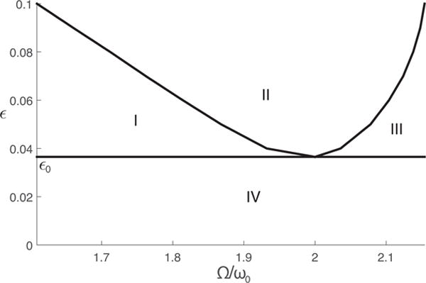
Transition curves of a periodically forced SIR model. Parameters of the SIR model are shown in Table 1. The parameter plane is separated into four regions based on different behaviors of the periodic solutions. In region I, three solutions coexist, including two stable solutions and one unstable solution. In region II, an unstable trivial solution and a stable non-trivial solution coexist. In region III and region IV, only a trivial solution exists.

When ε is below a certain threshold ε₀ and the system falls into region IV, there will be no resonance. In this case, the trivial solution is the only solution, and the system response oscillates at frequency Ω. Time series and phase plane plots from this region are shown in Fig. 3 (e) and (j).

Figure 3.

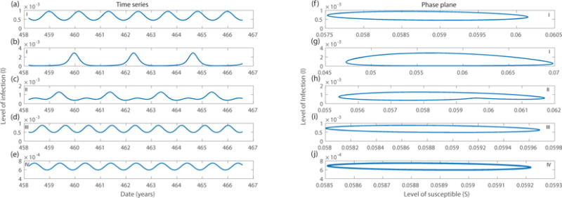
Time series (left column) and phase plane (right column) plots for an SIR model when parameters ε and Ω/ω₀ fall into different regions separated by transition curves. The corresponding region of parameters are shown on the plot. The same set of parameters is used in the first and second rows, showing two coexisting stable solutions. Parameter values of ε and Ω/ω₀ are as follows: first and second rows, ε = 0.05, Ω/ω₀ = 1.8; third row, ε = 0.06, Ω/ω₀ = 2.1; fourth row, ε = 0.02, Ω/ω₀ = 2.1; final row, ε = 0.06, Ω/ω₀ = 2.3.

When ε is above the threshold ε₀, whether the trivial solution (A = B = 0) is stable depends on both the amplitude of seasonality ε and the detuning factor k. The rest of the ε − Ω/ω₀ plane can be further divided into three regions (regions I, II and III) as shown in Fig. 2.

When the detuning factor is positive and above a certain threshold, the system will fall into region III where only the trivial solution A = B = 0 exists. The system again oscillates at frequency Ω as shown in Fig. 3 (d) and (i). In this case, only small annual cycles can be observed.

For systems belonging to region II, two solutions exist. The trivial solution A = B = 0 is unstable. Thus, the system will always exhibit resonance, oscillating at frequency $\frac{\mathrm{\Omega }}{2}$ with nonzero values for A and B, which corresponds to biennial cycles as shown in Fig. 3 (c) and (h).

As the detuning factor becomes smaller, system goes into region I where there are three coexisting solutions. The trivial solution is stable in this region, coexisting with one stable and one unstable resonance solutions. Time series and phase plane plots of the stable and unstable solutions are shown in Fig. 3 (a), (f) and (b), (g). In region I, annual cycles and biennial cycles are separated by an unstable solution. Transitions from one solution to another can be triggered by perturbations in the state variables without changing the parameter. This suggests that transitions from annual cycles to biennial cycles might be caused by suddenly introducing a large enough amount of infectious individual to the region.

Biennial cycles can be observed in an annual forced SIR model in different parameter regions. Transitions from annual cycles to biennial cycles can thus be triggered in different ways. Using the transition curve obtained from analysis, we can explore the behavior of a periodically forced SIR model and the transitions between different behaviors in more detail.

3. Parametric analysis

The stability of trivial linear solution and the existence of non-trivial solution depends on the amplitude of seasonality ε and on the natural frequency of the system ω₀. Because natural frequency is affected by the transmission rate β, the recovery rate γ and the death-birth rate μ, the transition from trivial linear solution (one year cycle) to non-trivial solution (biennial cycle) can be triggered by changes in any of these parameters.

In previous research, it was observed that transition from annual cycles to biennial cycles (referred to as period doubling bifurcation) could be triggered by increasing the amplitude of seasonality ε [14]. It was pointed out also that the transition from large amplitude biennial cycles to small amplitude oscillations can be caused by decreasing the transmission rate β, or increasing the birth rate [1]. In this section, we show that all transitions observed in previous studies are caused by crossing transition curves in the ε − Ω/ω₀ plane due to changes in parameters. Effects of changing the amplitude of seasonality ε the transmission rate β and the birth rate are revisited both analytically and numerically. Results from both analyses are compared to show the accuracy of the approximate solution obtained from the analysis. The influence of other parameters, such as the recovery rate γ is also studied.

3.1. Amplitude of seasonality ε

Increasing the amplitude of seasonality ε can bring the system from region IV to region II when the driving frequency Ω is close to twice the natural frequency ω₀ as shown in Fig. 2. When system is in region IV, the trivial linear solution is stable. Thus, the system shows annual cycles with small amplitude. When ε is larger, the system transitions from annual cycles to biennial cycles. Fig. 4 shows the change in the maximum level of infection in this process. An abrupt increase in the amplitude of infectious population accompanies the period-doubling phenomenon. Results from both analytical and numerical analyses are compared to show the accuracy of the approximation solution obtained from analytical analysis.

Figure 4.

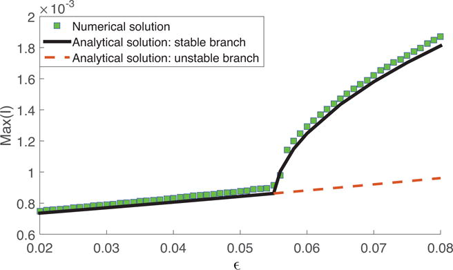
Maximum level of infection plotted against the amplitude of seasonal forcing ε as the system transitions from a non-resonance region (region IV) to a resonance region (region II) by increasing ε. The solid black line gives the stable branch of the analytical solution; the red dashed line gives the unstable branch of the analytical solution; the green squares show the results from numerical simulation. Parameters are same as in Table 1.

It is worth pointing out that the threshold ε₀ for the non-trivial solution to exist can be lower when the driving frequency Ω is closer to twice the natural frequency ω₀ of the system. The threshold is lowest when Ω is exactly 2ω₀. This threshold can be much lower than originally believed, and it shows that large biennial outbreaks are more likely to happen when the natural frequency is closer to 1/(2 years).

3.2. Transmission rate β

When ε is fixed, decreasing the transmission rate β causes a simultaneous shift of transition curve and of the natural frequency. Fig. 5 shows that decreasing β with fixed γ lowers and broadens the transition curve. Thus, it becomes easier to trigger parametric resonances. ω₀ decreases as β decreases because ${\omega }_0=\sqrt{-{\mu }^2{R}_0^2+4\mu (\beta -\gamma -\mu )}$ and $-{\mu }^2{R}_0^2$ is much smaller than μ(β − γ − μ). Because Ω is fixed as 1/year, the decrease in β actually takes the system from left to right in the parameter space in Fig. 5. Therefore, the transition may not take place as the transmission rate decreases, depending on the relative relationship between the position of the system in the parameter space and the transition curve.

Figure 5.

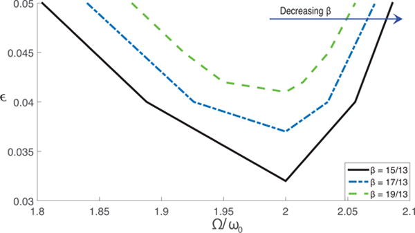
Change of the transition curve for parametric resonance as the transmission rate β is increased. The solid black line, blue and green dashed lines give the transition curve obtained using transmission rates of 15/13, 17/13 and 19/13, respectively. Parameters other than the transmission rate are the same as in Table 1.

Consider a scenario where the system starts in region I, where there are three coexisting solutions. As the transmission rate decreases, the system passes region II and finally reaches region III. In this process the solution transitions from large amplitude biennial cycles to annual cycles, as shown in Fig. 6. Analytical solutions are compared with numerical solutions (obtained using a shooting method [23, 24, 25]). Figure 6 shows that the analytical solution predicts the stable branch of the solution well. However, the unstable branch in region I has poor agreement with the numerical solution. In fact, region I can be further divided into two regions according to numerical simulation, because as β becomes larger than certain value, numerical simulation can only find one unique solution instead of three coexisting solutions. The discrepancy between analytical solutions and numerical simulations can be explained by the failure of the MMS approximation as the amplitude or the detuning factor becomes large.

Figure 6.

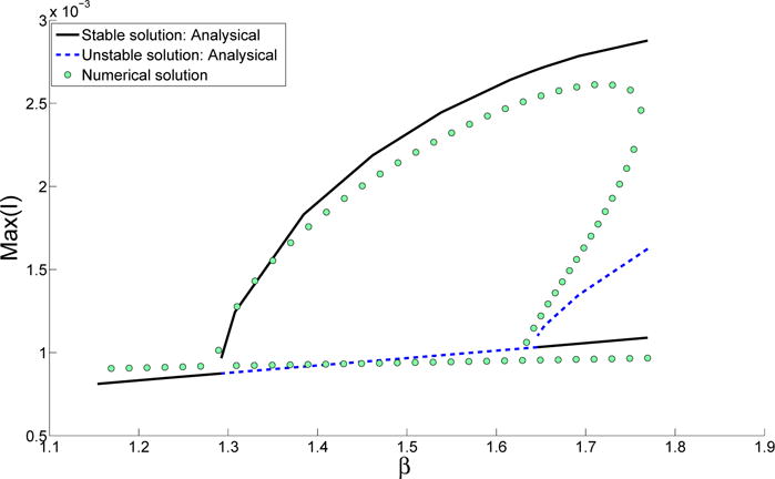
Maximum level of infection plotted against the transmission rate β as the system transitions from region I to region II and finally to region III by decreasing β. The black solid line shows the stable branch of the analytical solution; the dashed blue line shows the unstable branch of the analytic solution; the green circles show the results from the numerical simulations. Parameters other than the transmission rate are the same as in Table 1.

3.3. Birth rate

Changes in birth rate can also move the system from one section to another, causing changes on the periodicity of epidemics [1, 26, 27, 28]. It has been noted in [29] that for measles dynamics typically annual cycles take place when birth rate is high.

Changes in the birth rate are dynamically equivalent to changes in the transmission rate for SIR-based models as pointed out in [1]. Therefore, consider a scenario where the system starts in region II (similar to Section 3.2). The only stable solution in region II is the biennial solution. As the birth rate increases, the system shifts from region II and reaches region I. In this process the solution transitions from large amplitude biennial cycles to annual cycles, as shown in Fig. 7.

Figure 7.

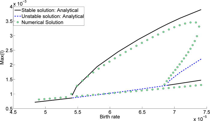
Maximum level of infection plotted against the birth rate as the system transitions from region I to region II and finally to region III by decreasing the birth rate. The black solid line shows the stable branch of the analytical solution; the dashed blue line shows the unstable branch of the analytic solution; the green circles show the results from the numerical simulations. Parameters other than the birth rate are the same as in Table 1.

Despite the limited accuracy of the analytical MMS method in predicting the unstable branch, this method still provides useful insight into biennial cycles. For the case of measles, the change from large biennial cycles to irregular annual cycles in the last century can be explained by the transition from one region to another induced by changes in the birth rate and vaccination rates.

3.4. Recovery rate γ

The recovery rate γ determines the average infectious period, which can be estimated from epidemiological data. The recovery rate typically does not change significantly over time, and it has a similar effect on the natural frequency of the system as the transmission rate. Thus, we do not focus on the effects of changing recovery rate over time on the transition from annual cycles to biennial cycles. However, different diseases have different transmission rate and recovery rate, which results in a different thresholds ε₀ for the transition. By analyzing cases with the same transmission rate β yet different recovery rates, we understand what are the effects of recovery rate on the threshold.

Fig. 8 shows that with the same transmission rate, increasing recovery rate lowers the threshold for parametric resonance. When recovery rate γ becomes larger than 0.14, the threshold can be as low as 0.01, which is much lower than originally believed [3, 15, 20]. The situation is opposite with the transmission rate. For constant recovery rate and increasing the transmission rate, there will be an increase in the threshold. Therefore, it can be concluded that systems with larger recovery rates and small transmission rates have smaller threshold for parametric resonance even if they might have similar natural frequencies.

Figure 8.

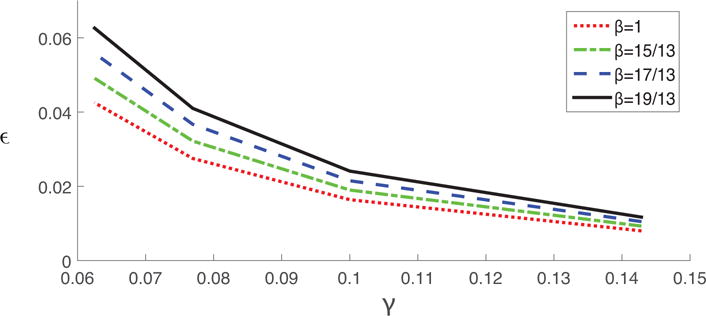
Threshold for amplitude of seasonal forcing ε plotted against recovery rate γ. The threshold ε₀ is defined as the maximum of region IV as shown in Fig. 2. All four lines from top to bottom are obtained using transmission rate values of 19/13, 17/13, 15/13, and 1, respectively.

4. Effects of stochasticity

We have observed that small changes in the periodic forcing, either amplitude or frequency, can cause a qualitative change in the behavior of the system. Stochasticity can have such disproportionate effects also. To understand the role of stochasticity in triggering parametric resonance, when periodic forcing and weak noise are present at the same time, the SIR model is transformed into a stochastic SIR model as in [30]

$$\begin{array}{l}dS(t)=(\mu -\beta S(t)I(t)-\mu S(t))dt-\sigma S(t)I(t)dW(t),\\ dI(t)=(\beta S(t)I(t)-(\mu +\gamma )I(t))dt+\sigma S(t)I(t)dW(t),\\ dR(t)=(\mathrm{\lambda }I(t)-\mu R(t))dt,\end{array}$$ (21)

where σ is a positive constant, and W is a standard Wiener process over the time interval [0 T]. The model is solved numerically using the Euler-Maruyama method, and the results for different noise level are shown in Fig. 9. This model is chosen because it enables us to study how different levels of stochasticity can cause different types of behavior of the system. When σ = 0, no noise is added to the system, so the system remains at the trivial solution, oscillating at frequency Ω with a relatively low amplitude. However, as the level of noise increases, the system starts switching between annual cycles and biennial cycles. After noise reaches a certain level, such as σ = 0.2, the system stabilizes on biennial cycles with a much larger amplitude.

Figure 9.

Stochastic simulations of an SIR model with periodic forcing and white noise. Levels of noise are 0, 0.05, 0.1 and 0.2 respectively for (a), (b), (c) and (d). All simulations start from the same initial condition. After a certain amount of simulation time, data are collected for 20 years to show different patterns under different levels of noise.

When the amplitude of the periodic forcing is close to the threshold, even weak noise can force the system out of the basin of attraction of the annual cycles. Therefore, the presence of stochasticity can significantly increase the amplitude of the system response by triggering the parametric resonance. In addition, the threshold of amplitude of periodic forcing can be further reduced when the system is accompanied by noise. This is important for understanding the effects of parametric resonance in epidemiology.

5. Conclusions

An analysis based on the method of multiple scales (MMS) is carried out to study a classic SIR model with periodic forcing. Analytical approximate solutions were obtained to show that parametric resonance can occur through the interaction between nonlinearity and seasonal forcing. The results reveal that large amplitude epidemics can take place if the system is moved into a resonance regime in the parameter plane by the change of any one of its parameters. This analysis can be extended to more complex epidemiological or biological models where more variables or other kinds of nonlinearity are present.

An important contribution of this analysis is that it shows that small order parametric excitations can synchronize with the system response, and trigger an order 1 parametric resonance. When parametric resonance is triggered, the excitation drives the growth of the biennial cycles until it is constrained by the nonlinearity.

This analysis also reveals that not only the amplitude of the parametric excitation, but also the relationship between natural frequency and excitation frequency matters. Therefore, all parameters can have an impact on triggering parametric resonance by changing the natural frequency of the system and changing the threshold of seasonality. Thus, this analysis unifies past research about the effects of different parameters on the biennial cycles of measles [1, 13, 14, 15]. It is also important to notice that large recovery rates and smaller transmission rates can lead to lower thresholds for parametric resonance.

Stochasticity also plays an important part in the dynamics. In particular, we showed numerically that stochasticity can trigger parametric resonance even when the system is in the non-resonance regime of the parameter space. This is because the stochasticity also contains components with the same frequency as the parametric excitation. When the intensity of stochasticity reaches a certain level, it can in fact push the system into the resonance regime, and induce the large amplitude biennial cycles.

The dynamics of childhood infectious disease is affected by the interplay between nonlinearity, periodic forcing and stochasticity. Through this analysis, the interaction between nonlinearity and periodic forcing as the source of instability is can be understood more clearly. More importantly, this work introduced for the first time perturbation methods such as the MMS to epidemiological models, and shows the considerable benefits of this approach. For example, it is much easier and more informative to study the effects of different parameters on the behavior of the system analytically rather than numerically. This type of methods can be applied to more sophisticated, higher dimensional epidemiological models, such as SIR model with multiple pathogens or pathogen strains [31], or spatial heterogeneity [32, 33]. In those cases, an analytical expression of the transition curve and the resonance peak as a function of the parameters can be quite useful [5].

References

- 1.Earn DJ, et al. A simple model for complex dynamical transitions in epidemics. Science. 2000;287(5453):667–670. doi: 10.1126/science.287.5453.667. [DOI] [PubMed] [Google Scholar]
- 2.Altizer S, et al. Seasonality and the dynamics of infectious diseases. Ecology Letters. 2006;9(4):467–484. doi: 10.1111/j.1461-0248.2005.00879.x. [DOI] [PubMed] [Google Scholar]
- 3.Keeling MJ, Rohani P. Modeling infectious diseases in humans and animals, Princeton University Press. 2008 [Google Scholar]
- 4.Anderson RM, May RM, Anderson B. Infectious diseases of humans: dynamics and control, Oxford University Press. 1992 [Google Scholar]
- 5.Jon Greenman MK, Boots M. External forcing of ecological and epidemiological systems: A resonance approach. Physica D: Nonlinear Phenomena. 2004;190(1):136–151. [Google Scholar]
- 6.Fine PE, Clarkson JA. Measles in england and walesi: An analysis of factors underlying seasonal patterns. International Journal of Epidemiology. 1982;11(1):5–14. doi: 10.1093/ije/11.1.5. [DOI] [PubMed] [Google Scholar]
- 7.Stone L, Olinky R, Huppert A. Seasonal dynamics of recurrent epidemics. Nature. 2007;446(7135):533–536. doi: 10.1038/nature05638. [DOI] [PubMed] [Google Scholar]
- 8.Bolker BM, Grenfell BT. Chaos and biological complexity in measles dynamics, Proceedings of the Royal Society of London B. Biological Sciences. 1993;251(1330):75–81. doi: 10.1098/rspb.1993.0011. [DOI] [PubMed] [Google Scholar]
- 9.Rand DA, Wilson HB. Chaotic stochasticity: a ubiquitous source of unpredictability in epidemics, Proceedings of the Royal Society of London B. Biological Sciences. 1991;246(1316):179–184. doi: 10.1098/rspb.1991.0142. [DOI] [PubMed] [Google Scholar]
- 10.Earn DJ, Rohani P, Grenfell BT. Persistence, chaos and synchrony in ecology and epidemiology, Proceedings of the Royal Society of London B. Biological Sciences. 1998;265(1390):7–10. doi: 10.1098/rspb.1998.0256. [DOI] [PMC free article] [PubMed] [Google Scholar]
- 11.Keeling MJ, Rohani P, Grenfell BT. Seasonally forced disease dynamics explored as switching between attractors, Physica D. Nonlinear Phenomena. 2001;148(3):317–335. [Google Scholar]
- 12.Alonso D, McKane AJ, Pascual M. Stochastic amplification in epidemics. Journal of the Royal Society Interface. 2007;4(14):575–582. doi: 10.1098/rsif.2006.0192. [DOI] [PMC free article] [PubMed] [Google Scholar]
- 13.Kuznetsov YA, Piccardi C. Bifurcation analysis of periodic seir and sir epidemic models. Journal of Mathematical Biology. 1994;32(2):109–121. doi: 10.1007/BF00163027. [DOI] [PubMed] [Google Scholar]
- 14.Aron JL, Schwartz IB. Seasonality and period-doubling bifurcations in an epidemic model. Journal of Theoretical Biology. 1984;110(4):665–679. doi: 10.1016/s0022-5193(84)80150-2. [DOI] [PubMed] [Google Scholar]
- 15.Dietz K. The incidence of infectious diseases under the influence of seasonal fluctuations. Mathematical Models in Medicine. 1976:1–15. [Google Scholar]
- 16.Black AJ, McKane AJ. Stochastic amplification in an epidemic model with seasonal forcing. Journal of Theoretical Biolog. 2010;267(1):85–94. doi: 10.1016/j.jtbi.2010.08.014. [DOI] [PubMed] [Google Scholar]
- 17.Kampen V, Godfried N. Stochastic processes in physics and chemistry, Elsevie. 1992 [Google Scholar]
- 18.Nayfeh AH, Mook DT. Nonlinear Oscillations. John Wiley & Sons; 2008. [Google Scholar]
- 19.Nayfeh AH. The response of single degree of freedom systems with quadratic and cubic non-linearities to a subharmonic excitation. Journal of Sound and Vibration. 1983;89:457–470. [Google Scholar]
- 20.Hethcote HW, Levin SA. Periodicity in epidemiological models. Applied mathematical ecology. 1989:193–211. [Google Scholar]
- 21.Halberg F, et al. Transyears: new endpoints for gerontology and geriatrics or confusing sources of variability?, The Journals of Gerontology Series A. Biological Sciences and Medical Sciences. 2004;59(12):1344–1347. doi: 10.1093/gerona/59.12.1344. [DOI] [PubMed] [Google Scholar]
- 22.Rand R. Lecture notes on nonlinear vibrations (version 52) 2005 Available from: http://www.tam.cornell.edu/randdocs/nlvibe52.pdf.
- 23.Sundararajan P, Noah ST. Dynamics of forced nonlinear systems using shooting/arc-length continuation methodapplication to rotor systems. Journal of vibration and acoustics. 1997;119(1):9–20. [Google Scholar]
- 24.Ribeiro P. Non-linear forced vibrations of thin/thick beams and plates by the finite element and shooting methods. Computers & structures. 2004;82(17):1413–1423. [Google Scholar]
- 25.Von Groll G, Ewins DJ. The harmonic balance method with arc-length continuation in rotor/stator contact problems. Journal of sound and vibration. 2001;241(2):223–233. [Google Scholar]
- 26.Cummings DA, et al. The impact of the demographic transition on dengue in thailand: insights from a statistical analysis and mathematical modeling. PLoS Med. 2009;6(9):e1000139. doi: 10.1371/journal.pmed.1000139. [DOI] [PMC free article] [PubMed] [Google Scholar]
- 27.Althouse BM, et al. Synchrony of sylvatic dengue isolations: a multi-host, multi-vector sir model of dengue virus transmission in senegal. PLoS Negl Trop Dis. 2012;6(11):e1928. doi: 10.1371/journal.pntd.0001928. [DOI] [PMC free article] [PubMed] [Google Scholar]
- 28.Broutin H, et al. Impact of vaccination and birth rate on the epidemiology of pertussis: a comparative study in 64 countries, Proceedings of the Royal Society of London B. Biological Sciences. 2010:rspb20100994. doi: 10.1098/rspb.2010.0994. [DOI] [PMC free article] [PubMed] [Google Scholar]
- 29.McLean AR, Anderson RM. Measles in developing countries part i. epidemiological parameters and patterns. Epidemiology and infection. 1988;100(01):111–133. doi: 10.1017/s0950268800065614. [DOI] [PMC free article] [PubMed] [Google Scholar]
- 30.Tornatore SMBE, Vetro P. Stability of a stochastic sir system, Physica A. Statistical Mechanics and its Applications. 2005;354:111–126. [Google Scholar]
- 31.Kamo M, Sasaki A. The effect of cross-immunity and seasonal forcing in a multi-strain epidemic model. Physica D: Nonlinear Phenomena. 2002;165(3):228–241. [Google Scholar]
- 32.Jansen VA. The dynamics of two diffusively coupled predatorprey populations. Theoretical Population Biology. 2001;59(2):119–131. doi: 10.1006/tpbi.2000.1506. [DOI] [PubMed] [Google Scholar]
- 33.Bernd Blasius AH, Stone L. Complex dynamics and phase synchronization in spatially extended ecological systems. Nature. 1999;399(6734):354–359. doi: 10.1038/20676. [DOI] [PubMed] [Google Scholar]
Associated Data
This section collects any data citations, data availability statements, or supplementary materials included in this article.