The Scandinavian Fantasy: The Sources of Intergenerational Mobility in Denmark and the US

Abstract

This paper examines the sources of differences in social mobility between the US and Denmark. Measured by income mobility, Denmark is a more mobile society, but not when measured by educational mobility. There are pronounced non‐linearities in income and educational mobility in both countries. Greater Danish income mobility is largely a consequence of redistributional tax, transfer, and wage compression policies. While Danish social policies for children produce more favorable cognitive test scores for disadvantaged children, they do not translate into more favorable educational outcomes, partly because of disincentives to acquire education arising from the redistributional policies that increase income mobility.

1.

The American Dream is now spoken with a Scandinavian accent. (Washington's Blog, 2014)

I. Introduction

Policy analysts around the world point to Scandinavia as a model for reducing inequality and promoting intergenerational mobility (see, e.g., Baily, 2016). By conventional measures, social mobility by income is much higher there than in the US.

In this paper, we use rich Danish data to explore the sources of these differences in social mobility. By all accounts, Denmark is a prototypical Scandinavian welfare state. Lessons learned from Danish data apply to Scandinavia more generally.

Our investigation reveals some surprises and apparent contradictions. The literature on Danish social mobility by income is surprisingly sparse and uses only a limited number of measures of income. One contribution of this paper is to demonstrate that the choice of the measure of income used matters greatly in determining the relative social mobility of the US and Denmark.

The standard measure of intergenerational mobility is based on the intergenerational elasticity (IGE): a regression coefficient showing the percentage change in a child's income associated with a percentage change in parental income. We show that estimated IGEs depend greatly on the measure of income used and that estimated IGEs vary with the level of income. US social mobility is low (absolutely and compared to Denmark) for children from high‐income families.

Popular discussions of the benefits of the Scandinavian welfare state point to its generous support of childcare and education relative to the US as major determinants of its greater social mobility. In Denmark, college tuition is free, there is ready access to childcare, pregnancy‐leave policy is generous, and there is virtually universal free pre‐kindergarten. Yet, despite these stark policy differences, the influence of family background on educational attainment is surprisingly similar in the two countries. Levels of intergenerational educational mobility are about the same. At higher levels of family income, educational mobility is lower in both countries.

In both countries, cognitive and non‐cognitive skills acquired by age 15 are more important for predicting educational attainment than parental income. The more child‐generous Danish welfare state produces much more favorable distribution of cognitive skills for disadvantaged Danish children compared to their counterparts in the US. The similarity of the influence of family background on educational attainment in the two countries, despite the more favorable distribution of test scores for Danish disadvantaged children, arises in part from the compression of the wage scale and the generous levels of social benefits that discourage Danish children from pursuing further schooling. In addition, the generosity of the Danish welfare state does not prevent sorting of children into neighborhoods and schools on the basis of family background, which appears to benefit the more advantaged.

Scandinavia invests heavily in child development and boosts the test scores of the disadvantaged. It then undoes these beneficial effects by providing weak labor market incentives. Better incentives to acquire skills would boost Danish educational mobility. Stated differently, the greater incentives to acquire education in the US labor market tend to offset its less favorable investments in the cognitive skills of disadvantaged children. In addition, while the Danish welfare state promotes equality of opportunity compared to the US, many barriers remain. There are large skill gaps between the children of the advantaged and the children of the disadvantaged, during early and late childhood. Residential sorting across neighborhoods and schools is strong.

This paper proceeds in the following way. In Section I., we analyze income mobility in Denmark and the US. We examine the sensitivity of estimated income IGEs to alternative measures of income. We examine the sources of differences in income mobility. We also report non‐parametric estimates of income mobility. In Section Non‐Linear Intergenerational Income Elasticities, we examine the relationship between schooling attainment, measures of family financial resources, cognitive and non‐cognitive skills of children at age 15, family background (education and home environment), and measures of schooling quality. We report surprisingly similar effects of family influence on educational attainment in both societies. We show a link between welfare benefits and educational attainment in Denmark. We discuss the role of neighborhood sorting on child educational attainment. In Section Neighborhood Sorting of Children by Family Background, we qualify our analysis. We conclude in Section IV..

II. Income Mobility

In this section, we explore alternative measures of intergenerational income mobility. Different measures of income convey very different impressions of social mobility. We show how the levels of transfers, the mapping of education to income, the levels and progressivity of taxation, and income inequality differ between the US and Denmark. All four factors affect estimates of income mobility.

We report estimates of non‐linear (NL) IGEs for both countries. We find different patterns depending on which income measure we consider. Differences favoring Denmark appear at the lowest and the highest levels of income.

Data

US Data

We use two US data sources. We use Panel Study of Income Dynamics (PSID) data for our main analysis of intergenerational income mobility. We measure parental income using a nine‐year average from the child's 7th to 15th year.¹ Child income is measured as income at ages 34–41 down to ages 30–35 for the 1972–1978 birth cohorts. In our main analysis, we only consider individuals with positive incomes. See Section F in the Online Appendix (https://cehd.uchicago.edu/scandinavian-appendix) for more details.

As the sample size for the PSID data is small (relative to the Danish data), we use the March Current Population Survey (CPS; 1968–2014) from the Integrated Public Use Microdata Series (IPUMS)² when we analyze US income distributions. The sample consists of civilian, non‐institutionalized citizens. We use parents in 1987 and individuals aged 36–38 in 2011.

Danish Data³

For Denmark, we use the full population register data on the entire cohorts born in 1973–1975. We discard individuals who migrate (or whose parents migrate), individuals for whom we have no identification of the father or mother (around 2 percent), and individuals with negative incomes (averaged over the period where we measure income). Parental income is measured as a nine‐year average from when the child is 7–15 years of age, and the child's income is measured at ages 35–37, 36–38, and 37–39 for the 1975, 1974, and 1973 cohorts, respectively. The full sample size is 166,359, and once we restrict to positive incomes the sample is reduced to 149,190 individual parent–child matches.⁴

In the Online Appendix, Table A23 provides the definitions of the various income measures we consider, Table A1 summarizes income levels for the US and Denmark by different quantiles and income measures, and Figure A1 depicts the distributions. Table A1 and Figure A1 in the Online Appendix show that incomes in Denmark are more compressed than incomes in the US. There is a large low‐income group in the US that virtually does not exist in Denmark (Forslund and Krueger, 1997; Aaberge et al., 2002; Corak, 2013).⁵ In the next section, we show that cross‐sectional differences in income distributions between Denmark and the US are an important source of higher income mobility in Denmark than in the US.

Linear Intergenerational Income Elasticities

There is a large literature investigating the association between parents' and children's income.⁶ The modal statistic used to study income mobility is the IGE of income ${\beta }^{IGE}$:

$$ln\left(Y^C\right)=\alpha +{\beta }^{IGE}ln\left(Y^P\right).$$ (1)

The father/son or parent/child IGE is generally found to be much higher in the US than in Denmark. Estimates generally lie between 0.3 and 0.5 in the US and around 0.1 to 0.2 in Denmark (Björklund and Jäntti, 2011; Blanden, 2013; Mazumder, 2005; Solon, 2002). There is a similar range for rank–rank associations. Boserup et al. (2013) and Chetty et al. (2014) estimate this to be 0.18 in Denmark and 0.34 in the US, respectively. Based on these estimates of the income IGE, Scandinavia is portrayed as a land of opportunity.⁷

Cross‐country differences in estimated IGEs of income can arise for a multitude of reasons that we attempt to capture using different income measures. One measure proxies transmission of total individual income potential with wage earnings, capital income, and profits. Another proxies transmission of total income including public transfers (but not the impact of in‐kind transfers). A third measure introduces the effects of the progressivity of the taxation on income mobility. A fourth measure, wage earnings, proxies intergenerational transmission of earnings‐potential rewarded in labor market – differences arise, in part, from differences in returns to education.

A further source of differences in estimated IGEs arises from differences in levels and trends in cross‐sectional income inequality.⁸ We put this issue aside for now, and investigate it in the following subsection.

Table 1 shows estimated intergenerational income elasticities for similar income measures in Denmark and the US. The odd‐numbered columns report estimates for Denmark. The even‐numbered columns report the corresponding estimates for the US.

Table 1.

IGE estimates with different income measures: Denmark and the US

	Gross income excl.		Gross income incl.		Wage earnings		Wage earnings and		Net‐of‐tax total
	public transfers		public transfers				public transfers		gross income
	Denmark	US	Denmark	US	Denmark	US	Denmark	US	Denmark
	(1)	(2)	(3)	(4)	(5)	(6)	(7)	(8)	(9)
Estimated IGE	0.352***	0.312***	0.271***	0.446***	0.083***	0.289***	0.063***	0.419***	0.221***
	(0.004)	(0.055)	(0.003)	(0.054)	(0.003)	(0.044)	(0.003)	(0.058)	(0.003)
Observations	149,190	621	149,190	621	149,190	621	149,190	621	149,190

Notes: This table shows coefficients (${\beta }^{IGE}$) and standard errors from regressions of child log income on parent log income for Denmark and the US. For Denmark, we use full population register data for children born in the period 1973–1975, and for the US we use PSID data for children born in the period 1972–1978. For Denmark, parental income is measured as a nine‐year average from the child's 7th to 15th year, and the child's income is measured at ages 35–37, 36–38, and 37–39 for the 1975, 1974, and 1973 cohorts, respectively. For the US, parental income is measured as a nine‐year average from the child's 7th to 15th year, and the child's income is measured as last‐year income at ages 34–41, 33–40, 32–39, 31–38, 30–37, 30–36, and 30–35 for the 1972, 1973, 1974, 1975, 1976, 1977, and 1978 cohorts, respectively. The columns are based on the following: column 1, for Denmark, all taxable income including wage earnings, profits from own business, capital income, and foreign income excluding all public transfers (both taxable and non‐taxable); column 2, for the US, all taxable income including earnings (payroll income from all sources, farm income, and the labor portion of business income), asset income (such as rent income, dividends, interest, income from trust and royalties, and asset income from business), and private transfers (such as income from alimony, child support, and help from relatives and others); column 3, for Denmark, all taxable income including wage earnings, public transfers, profits from own business, capital income, and foreign income; column 4, for the US, all taxable income including earnings, asset income, private transfers and public transfers (such as social security income, SSI, TANF, ETC, other welfare income, retirement, pension, unemployment, and workers compensation); column 5, for Denmark, taxable wage earnings and fringes, labor portion of business income, and non‐taxable earnings, severance pay, and stock‐options; column 6, for the US, payroll income from all sources (such as wages and salaries, bonus, overtime income, tips, commissions, professional practice, market gardening, additional job income, and other labor income), farm income, and labor portion of business income; column 7, for Denmark, taxable wage earnings and fringes, labor portion of business income, and non‐taxable earnings, severance pay, and stock‐options, plus taxable and non‐taxable public transfers (social assistance, unemployment benefits, labor market leave, sick leave assistance, labor market activation, child benefits, education grants, housing support, early retirement pension, disability pension, and retirement pension); column 8, for the US, payroll income from all sources, farm income, labor portion of business income, and public transfers; column 9, for Denmark, total gross income minus all final income taxes paid in given year (note we do not have information on individual net‐of‐tax income from the PSID). ⁺ p < 0.1; *p < 0.05; **p < 0.01; ***p < 0.001.

Column 1 shows that the estimated IGE based on gross income, excluding public transfers, is 0.352 for Denmark. This estimate is much higher than estimates reported in the literature, which use wage earnings, earnings, or income including public transfers. The corresponding estimate for the US is 0.312. The difference between the two estimates is not statistically significant. The third and fourth columns show that the estimated IGE for Denmark drops by around 20 percent to 0.271 when public transfers are included in the measure of income. This decrease illustrates the important role of redistribution in Denmark. For the US, the corresponding estimate jumps to 0.446, bringing us close to the estimate reported in Solon (1992) and Chetty et al. (2014) (see Table A1 in the Appendix). Comparing the estimate in column 3 in Table 1 to that of column 9 in the same table, we see that adding taxation reduces the Danish IGE estimate further. Unfortunately, we do not have the data required to estimate the corresponding IGE for the US.⁹

When we focus on wage earnings alone in columns 5 and 6, the estimated IGE for Denmark drops dramatically to 0.083, while the corresponding US estimate is 0.289. Finally, adding public transfers to wage earnings results in an even larger gap between the two countries. For wage earnings plus public transfers, the Danish IGE is 0.063 while the US estimate is 0.419.¹⁰

Our estimates for Denmark do not contradict the findings of the previous literature. Rather, they enrich our understanding of them. Measured by income potential (columns 1 and 2), we find that intergenerational mobility in Denmark is not significantly different from intergenerational mobility in the US. When we account for public transfers, estimates for the two countries diverge. Income mobility by this measure is substantially higher in Denmark than in the US. When we consider wage earnings alone or wage earnings inclusive of public transfers, we obtain estimates for Denmark reported in the previous literature with estimated IGEs around 0.1.

One should interpret cross‐country differences with great caution. There is no single best measure of the IGE. We do not claim that we have shown that levels of income mobility in the US and Denmark are alike or different. The conclusion from this analysis is that by accounting for transfers, wage compression, returns to education, and progressive income taxation, we can explain a substantial portion of the Denmark–US difference in associations between children's and parents' income.

In addition, several measurement problems discussed in the previous literature (see, e.g., Solon, 2004) might also affect estimated IGEs. Imputing zeros with an arbitrary value affects estimates. Censoring might also produce biased results, for example, by leaving out the long‐term unemployed from the analysis.¹¹ Table A5 in the Online Appendix reports the estimates corresponding to Table 1 when imputing zero incomes with $1,000. The table shows that estimated IGEs change for income categories that include many zeros (gross income excluding transfers and wage earnings).¹² Nevertheless, the overall patterns from Table 1 remain unchanged for Denmark. For the US, however, the PSID data are much more sensitive to the inclusion of zero and non‐reported incomes. In order to obviate the problems with zero income, analyses estimating relationships between children's and parents' ranks in their respective income distributions¹³ have recently been used (see Dahl and DeLeire, 2008; Chetty et al., 2014). We do not report results for rank–rank estimates in the main text and we refer readers to the Online Appendix.¹⁴ ${}^{,}$ ¹⁵

The Role of Inequality in Shaping the IGE

The cross‐country correlation between income mobility and income inequality has received a lot of attention in the past decade (Corak, 2006). Krueger (2012) calls this the “Great Gatsby curve”. In this subsection, we examine the mechanical relationship between estimated IGE and changes in inequality across generations. It follows from the definition of the IGE,

$${\beta }^{IGE}=corr[ln\left(Y^C\right),ln\left(Y^P\right)]\frac{sd[ln\left(Y^C\right)]}{sd[ln\left(Y^P\right)]},$$

that an increase in inequality from one generation to the next amplifies the estimate without affecting mobility measured by correlation coefficients. Hence, differences in inequality between generations and countries might generate differences in perceived income mobility.¹⁶

Table 2 shows how differences in variances drive estimates. The table shows the regression coefficients from Table 1 together with the correlation and intergenerational ratio of standard deviations below each coefficient. The table shows that, although not statistically significantly different, the intergenerational correlation for gross income excluding transfers in the US is above its Danish counterpart. It is the ratio of standard deviations that drives the Danish IGE to levels above the US. When public transfers are included in gross income, the correlation and ratio increase in the US, while in Denmark the ratio decreases and the correlation is roughly unchanged. These results also emphasize that transfers are more progressive and constitute a larger fraction of income in Denmark compared to the US. Furthermore, the table shows that the large increase in the estimated IGE for the US when public transfers are included, partly arises because transfers reduce inequality in parents' income while inequality in children's income is largely unaffected.¹⁷ When we focus on wage earnings alone, the correlation in Denmark drops from a level of 0.214 to 0.081, whereas in the US the intergenerational correlation remains unchanged.¹⁸ Table A5 in the Online Appendix presents a corresponding analysis imputing zero incomes with $1,000. The main difference for Denmark is that intergenerational correlations for gross income excluding transfers and wage earnings increase to 0.246 and 0.118, respectively, while the correlations for the remaining incomes measure remain largely unaffected. Hence, including individuals with zero incomes, there is a substantial reduction in the intergenerational correlation when we add transfers to gross income in Denmark.

Table 2.

Intergenerational correlations and inequality for different income measures: Denmark and the US

	Gross income excl.		Gross income incl.		Wage earnings		Wage earnings and
	public transfers		public transfers				public transfers
	Denmark	US	Denmark	US	Denmark	US	Denmark	US
	(1)	(2)	(3)	(4)	(5)	(6)	(7)	(8)
${\beta }^{IGE}$	0.352***	0.312***	0.271***	0.446***	0.083***	0.289***	0.063***	0.419***
${\rho }_{Child,Parents}\frac{sd\left(Child\right)}{sd\left(Parents\right)}$	$0.201\frac{0.860}{0.491}$	$0.268\frac{0.977}{0.840}$	$0.214\frac{0.375}{0.308}$	$0.318\frac{0.906}{0.645}$	$0.081\frac{1.004}{0.989}$	$0.256\frac{0.970}{0.860}$	$0.075\frac{0.561}{0.669}$	$0.280\frac{0.923}{0.615}$

Notes: This table shows coefficients (${\beta }^{IGE}$) and standard errors from regressions on parental log income on child's log income from Table 1, together with the correlation multiplied with the ratio of the standard errors ${\beta }^{IGE}={\rho }_{Child,Parents}(sd\left(Child\right)/sd\left(Parents\right))$ for Denmark and the US. ⁺ p < 0.1; *p < 0.05; **p < 0.01; ***p < 0.001.

From this analysis, we see that IGE estimates are sensitive not only to the income measures used, but also to inequality levels and changes. It is not meaningful to compare IGE estimates, when arbitrary large or small levels of inequality drive the estimates. In order to investigate this issue in greater depth, we conduct a further analysis showing the sensitivity of IGE estimates to adjustments for inequality.

We present regressions where we transform the different income distributions for Denmark to the corresponding income distributions for the US, holding income ranks fixed. Then, we place the US distribution in the Danish distribution. In the upper panel of Table 3, we present IGE estimates where quantiles of the Danish distributions – for parents (reported in the rows) and for children (reported in the columns) – are mapped into the equivalent income measures for the US for children born in the period 1973–1975 in 2011 with parents in the 1987 March CPS data. Figure A2(a) in the Online Appendix illustrates the transformation for wage earnings distributions. The child or parent with the nth total gross income rank in Denmark is assigned the total gross income level associated with the nth rank of total gross income for the US child or parent distribution. A similar transformation is used for total income excluding public transfers, total net‐of‐tax income, wage earnings, and wage earnings plus public transfers. Using this method, we illustrate what the Danish IGE would be for the different income measures, if Denmark had the same levels of inequality within generations as those found in the US.

Table 3.

IGE estimates with different income measures, imposing US income distribution on Danish distribution, and vice versa

	Gross income excl.		Gross income incl.		Net‐of‐tax total		Wage earnings		Wage earnings and
	public transfers		public transfers		gross income				public transfers
	Baseline	Transformed	Baseline	Transformed	Baseline	Transformed	Baseline	Transformed	Baseline	Transformed
	child	child	child	child	child	child	child	child	child	child
	inc. dist.	inc. dist.a	inc. dist.	inc. dist.	inc. dist.	inc. dist.	inc. dist.	inc. dist.	inc. dist.	inc. dist.
	(1)	(2)	(3)	(4)	(5)	(6)	(7)	(8)	(9)	(10)
Panel A: US distribution imposed on Danish distribution
Baseline parent	0.352***	0.435***	0.271***	0.600***	0.221***	0.392***	0.083***	0.071***	0.063***	0.104***
	(0.004)	(0.005)	(0.003)	(0.008)	(0.003)	(0.006)	(0.003)	(0.002)	(0.002)	(0.003)
Transformed parent	0.187***	0.230***	0.093***	0.213***	0.093***	0.168***	0.150***	0.138***	0.068***	0.124***
	(0.002)	(0.002)	(0.001)	(0.003)	(0.001)	(0.002)	(0.003)	(0.002)	(0.002)	(0.002)
Panel B: Danish distribution imposed on US distribution
Baseline parent	0.308***	0.207***	0.433***	0.186***			0.302***	0.247***	0.394***	0.177***
	(0.051)	(0.042)	(0.060)	(0.028)			(0.051)	(0.050)	(0.062)	(0.032)
Transformed parent	0.666***	0.501***	0.734***	0.337***			0.338***	0.304***	0.378***	0.186***
	(0.095)	(0.079)	(0.105)	(0.048)			(0.055)	(0.054)	(0.067)	(0.034)

Notes: This table shows coefficients (${\beta }^{IGE}$) and standard errors from regressions of child log income on parents' log income using the samples, variables, and income definitions detailed in the notes to Table 1. The columns labeled “Baseline child” show IGE of income where child's income distribution is unchanged. The columns labeled “Transformed child” show IGE of income where children's income distribution has been changed to fit the distributions of the corresponding income measures for the US in panel A and the corresponding income measures for Denmark in panel B. Rows labeled “Baseline parent” show IGE of income where parents' household income distribution is unchanged. Rows labeled “Transformed parent” show IGE of income where parents' household income distribution has been changed to fit the reported income distributions for corresponding income measures for the US in panel A and for Denmark in panel B. Number of observations: panel A, 149,190; panel B, 621. ⁺ p < 0.1; *p < 0.05; **p < 0.01; ***p < 0.001.

This is a radial transformation quantiles of Danish child income distribution mapped into quantiles of comparable measures of US distribution.

In the lower panel of Table 3, we do the opposite, which is illustrated in Figure A2(b) in the Online Appendix. In this case, quantiles of the US distributions are mapped into the equivalent income measures in 2010–2012 for Denmark for children born in the period 1973–1975 and their parents, using Danish register data. Hence, we illustrate what the US IGE would be for the different income measures, if the US had the same levels of inequality within generations as those found in Denmark.

The columns and rows labeled “Baseline” for both parents and children show the actual IGE coefficients from Table 1. The first line in the upper panel shows that if Danes born between 1973 and 1975 had the same income distribution as the corresponding US age cohorts, the Danish IGE estimates for gross income excluding transfers, including transfers, and net‐of‐tax would increase by 50–100 percent, whereas it would be unchanged for wage earnings. In the next thought experiment, we examine the consequences of giving Danish parents the same income distribution as US parents. Estimated IGEs would decrease. Transforming children's and parents' income distribution reduces IGEs by 30–50 percent when we consider the gross income measures, and increases IGEs by roughly 50–100 percent when we consider wage earnings and wage earnings plus transfers.

When we perform the equivalent exercise for the US, we naturally reach the opposite conclusion. Changing the income distribution of children while holding parents' income distributions fixed results in large reductions in the IGE, whereas changing income distributions for parents while holding children's income distributions fixed results in large increases in the IGE. Finally, by transforming both generations' income distributions, the IGE by gross income excluding transfers increases, the IGE for income measures including transfers decreases, and the IGE for wage earnings is unchanged.

Table 3 shows that IGEs in Denmark and the US are quite different when wage earnings and wage earnings plus transfers are used as measures of income. Estimated IGEs based on these two income measures are robust to the changes in inequality that we observe for both countries. For the remaining measures of income, the similarities between the IGEs in Denmark and the US are substantial and depend strongly on trends and levels in inequality.

The analyses presented in this section emphasize that levels of estimated income (im)mobility depend on the subjective evaluation of the reader. Not only do estimates vary by income measures, they are also affected by whether changing inequality is linked to mobility. For example, with a fixed correlation between children's and parents' income, doubling income inequality from one generation to the next clearly increases differences in income levels and the consumption possibilities between children from high‐income and low‐income families. Should the chosen measure of income mobility capture such change? Without specifying a social welfare function and a normative definition of fairness, this question does not have a clear answer.

Non‐Linear Intergenerational Income Elasticities

It is likely that any benefits from the Scandinavian welfare states accrue to the least advantaged. This is a feature that linear models of the IGE might fail to adequately capture. Thus, it is particularly interesting to analyze non‐linearities in the IGEs. Wage compression and the high level of redistribution via taxes and transfers only add weight to the relevance of considering possible non‐linearities.

Yet, few previous studies consider non‐linearities. Bratsberg et al. (2007) report that the relationship between the logarithm of child and parent income is convex in Denmark (and in Scandinavia more generally) and concave in the US for measures of wage earnings.¹⁹ They attribute this finding to higher mobility for individuals from low‐income families in Denmark than in the US. We replicate these findings in Figure A3 in the Online Appendix. However, as previously emphasized, results differ according to which income measure is used. In Denmark, for example, wage earnings of children and parents display a convex relationship, while for total gross income excluding public transfers the relationship is linear, or perhaps even concave.

We account for non‐linearities using local linear regressions. We estimate the NL‐IGE, ${\beta }^{IGE}[ln\left(Y_0^P\right)]$, where $Y_0^P$ is the income of the parent at Y ₀ and $Y^C$ is income of the child:²⁰

$$\begin{array}{ccc}& & \underset{\alpha [ln\left(Y_0^P\right)],\beta [ln\left(Y_0^P\right)]}{min}\stackrel{N}{\sum _{i=1}}{K}_{h_{\lambda }}\left(Y_0^P,Y_i^P\right)\hfill \\ & & \times {\left\{ln\left(Y_i^C\right)-\alpha \left[ln\left(Y_0^P\right)\right]-{\beta }^{IGE}\left[ln\left(Y_0^P\right)\right]ln\left(Y_i^P\right)\right\}}^2.\hfill \end{array}$$ (2)

It is feasible to estimate the NL‐IGEs using absolute income, thereby obviating the problem that ln(0) does not exist.²¹ However, the estimation of NL‐IGE using absolute income involves a trade‐off in terms of precision for high income levels due to the right tail of the income distribution. Doing so reduces the precision of estimates substantially. In order to be able to compare estimates from $10,000 to $125,000 and not just from $30,000 to $60,000 of parental incomes, we therefore report estimates using log income here. The corresponding point estimates using absolute income are very similar to the results shown in the main text and are reported in Figures A5 and A6 in the Online Appendix.

Figures 1 and 2 show plots of NL‐IGE estimates of log income, weighted with absolute income, without imputation for zero income for Denmark and the US. The vertical lines in the figures mark the 5th and 95th percentiles in the income distributions in the Danish data and the 5th and 95th percentiles for the US data. It should be noted that these estimates only allow us to infer local conclusions about mobility. A zero IGE estimate at a low level of income does not imply that going from rags to riches is likely. It only shows that a marginal movement up (or down) in income levels relative to parental income is just as likely as the status quo. The figures present estimates for the income ranges where the data allow us to make meaningful estimates (because there is very limited support for high incomes in the PSID).

Figure 1.

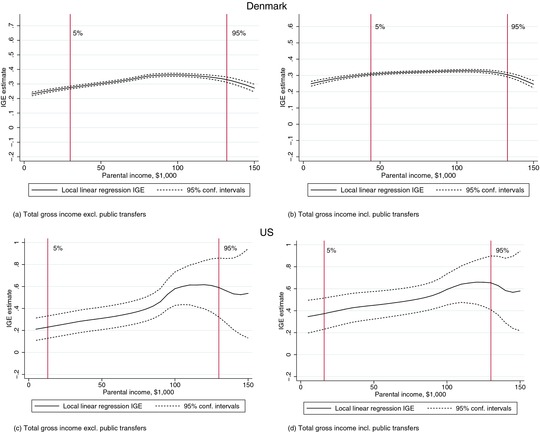
Local intergenerational income elasticity in Denmark and the US

Notes: The figures show estimated intergenerational income elasticities of wage income plus public transfers for Denmark (panels a and b) and the US (panels c and d). Panels (a) and (b) have been constructed using full population register data from Denmark, and panels (c) and (d) have been constructed using PSID data. The figures show local linear regression slopes of log of children's income on log of parental income. Local linear regressions are weighted using kernels of absolute income. Standard errors for panels (a) and (b) have been constructed from 50 bootstraps, and standard errors for panels (c) and (d) have been constructed from 1,000 bootstraps. The vertical lines indicate the 5th and 95th percentiles in the respective income distributions.

Figure 2.

Local intergenerational income elasticity in Denmark and the US (continued)

Notes: The figures show estimated intergenerational income elasticities of wage income plus public transfers for Denmark (panels (a), (b), and (e)) and the US (panels (c) and (d)). Panels (a), (b), and (e) have been constructed using full population register data from Denmark, and panels (c) and (d) have been constructed using PSID data. The figures show local linear regression slopes of log of children's income on log of parental income. Local linear regressions are weighted using kernels of absolute income. Standard errors for panels (a), (b), and (e) have been constructed from 50 bootstraps, and standard errors for panels (c) and (d) have been constructed from 1,000 bootstraps. The vertical lines indicate the 5th and 95th percentiles in the respective income distributions.

Figure 1 shows NL‐IGE estimates for gross income excluding public transfers and gross income including public transfers for Denmark and the US (Figures 1(a) and 1(b)). The elasticity goes from levels around 0.25 to almost 0.4 when parental income increases from $0 to $100,000. Thereafter, the estimates slowly decline and reach a level of around 0.1–0.2 at the 99th percentile of parental income. The corresponding results for the US (in Figures 1(c) and 1(d)) show that elasticities at low income levels closely correspond to those in Denmark, although they are imprecisely estimated. In the US, elasticities increase monotonically with parental income. At the 95th percentiles of parental gross income excluding and including public transfers, US intergenerational income elasticities are well above 0.5.

Figure 2 graphs NL‐IGE estimates for wage earnings and wage earnings plus public transfers for Denmark (panels a and b) and the US (panels c and d), and net‐of‐tax total gross (disposable) income for Denmark (panel e). Figures 2(a) and 2(b) show functional forms similar to those from Figures 1(a) and 1(b). Elasticities at low levels of income are approximately 0.1, or even lower, and increase monotonically until parental income reaches $110,000. After this point, the elasticities decrease. For the US, the figures also show a monotonic upward slope but with levels well above the Danish estimates at all points. Finally, elasticities for net‐of‐tax income in Denmark are initially flat at roughly 0.25 but go towards zero as parental income increases beyond the 99th percentile.

In order to obtain a more precise view of the cross‐country differences in NL‐IGEs, Figure 3 plots the differences between the US and the Danish elasticities across levels of parental income. From Figure 3(a), we see that income mobility in gross income excluding public transfers is roughly similar for family incomes up to $100,000. From this point onward, a gap emerges that – albeit imprecisely estimated – continues to increase. Income mobility by gross income excluding transfers is much lower in the US than in Denmark for top quartile family incomes, but not for families with low income. When transfers are added to income, as shown in Figure 3(b), the elasticities in the US are persistently above the Danish elasticities with a widening gap at high incomes. When we only consider wage earnings in Figure 3(c), the Danish IGE is around 0.2 lower than the US IGE across all parental income levels. This result also dovetails nicely with our argument about the importance of wage compression in Denmark, as opposed to the increasing return to education in the US, being key mechanisms behind the observed income mobility differences. Finally, Figure 3(d) shows that for wage earnings plus transfers, intergenerational income elasticities in Denmark are consistently below US levels. Here, the Danish IGE is around 0.35 lower than the US IGE at low income levels and 0.25 lower at high income levels. Hence, the largest difference between income mobility in Denmark and the US is now for the lowest family incomes.

Figure 3.

US–Denmark difference in local intergenerational income elasticity

Notes: This figure shows the US–Denmark difference in local intergenerational income elasticities from Figures 1 and 2. The figure shows the US IGE estimate minus the Danish estimate, such that a positive value indicates a larger IGE estimate for the US than for Denmark and a negative value indicates the opposite.

III. Educational Mobility by Family Background

In the previous section, we studied intergenerational income mobility across two countries and show that wage compression and tax/transfer policies are major determinants of cross‐country differences in mobility. Although the reward for education might be lower in Denmark, its generous support of education, support of childcare, and early education initiatives promote skill formation as measured by test scores among the disadvantaged.

Many point to the more generous educational and childcare policies in place in Denmark as a source of its greater social mobility (e.g., Sanders, 2013). We examine this claim and show that average educational mobility is remarkably similar across the two countries. We start by demonstrating the near‐universal participation in such programs in Denmark coupled with a lack of educational and income gaps compared to the US.²²

Figures 4(a) and 4(b) show the fraction of children enrolled in preschool programs at the age of 4 in the US and Denmark from 1995 to 2005.^{23 , 24} The figures show the overall rates, together with the rates for children for whom both parents have fewer than 12 years of schooling (less than high school) and for children for whom both parents have at least 15 years of schooling (college or more). The figures show that average preschool enrollment rates at age 5 were, on average, similar in the two countries in 1995. Since then, rates of participation have stagnated in the US and increased to a level close to full uptake in Denmark. Importantly, the figures also show large gaps in enrollment rates by parental education in the US, whereas there are no differences in Denmark.

Figure 4.

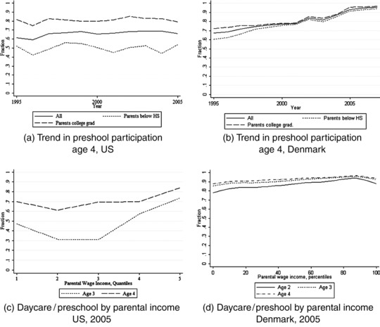
Daycare and preschool use

Notes: Panels (a) and (b) show the fractions enrolled in preschool at age 4 from 1995–2007 for all children and by parents' education. Panels (c) and (d) show the fractions in daycare/preschool by parental wage income rank within child cohort in 2005. The US figures are constructed from October CPS data, and the Danish figures are constructed from administrative register data.

Figures 4(c) and 4(d) show rates of daycare/preschool use at ages 2, 3, and 4 by parental wage income rank in 2005 in the two countries. Enrollment rates are lower in the US, trends in participation are flatter, and family income gradients for participation in the programs are steeper.

A few studies present causal evidence linking access to universal public childcare to improvements in skills in a Scandinavian context. Havnes and Mogstad (2011b) study a large expansion of childcare in Norway on long‐run outcomes. They find that daycare enrollment improves educational attainment and earnings, especially for children from low‐resource families.²⁵ Datta Gupta and Simonsen (2010, 2012) investigate the effects of home care, non‐parental/related family care (i.e., in a child‐minder's home), and public daycare in Denmark on socio‐emotional skills. Datta Gupta and Simonsen (2010) find that public daycare relative to family care increases socio‐emotional skills at age 7, while Datta Gupta and Simonsen (2012) suggest that the effects might fade at later ages.

There is an active body of literature in which the effectiveness of early childhood interventions in the US is investigated.²⁶ The evidence from many US programs might not be relevant to the current discussion, as the programs are often very intensive and target specific groups of children. Cascio (2009) reports that large‐scale, publicly funded childcare programs in the US are less effective than their Scandinavian counterparts. She suggests that low‐intensity programs crowd out other programs (e.g., Head Start) and divert funding from other public skill formation initiatives.

While the cited studies only investigate policy changes within a given country, they support the claim that increased early childhood investments, through universal public childcare, improve the skills of the least advantaged children and thus intergenerational skill mobility. The evidence for their effectiveness is supported by Figure 5, which shows distributions of Program for International Student Assessment (PISA) mathematics and reading scores in Denmark and the US in 2003.²⁷ The figure shows stark differences in the lower tails of PISA test scores. The lowest quartile in the US performs much worse than the lowest quartile in Denmark.

Figure 5.

Percentage of students at each proficiency level, PISA 2003

Source: OECD (2004).

Yet, despite the greater provision of early childhood education to low‐resource families in Denmark, the lack of any pecuniary costs of education in Denmark, the compressed skill distributions, and the association between educational attainment levels from one generation to the next are remarkably similar in Denmark and the US. Figure 6 shows the fraction of those aged 20–34 in (or with) a tertiary education, by parental educational attainment in Denmark, the US, and Norway. The figure shows that only 6–8 percent of individuals aged 20–34 who are enrolled in or have completed a tertiary education come from homes where both parents have not graduated from an upper secondary education. Generally, there are few differences in these percentages across the three countries. Figure A13 and Section B.2 (Figure A30) in the Online Appendix corroborate this evidence. Figure A13 shows that educational mobility in Denmark is not higher than in the US if we instead consider regression‐based coefficients relating children's and parents' educational attainment as reported in Hertz et al. (2008). Educational transitions across generations are very similar in the two countries for more recent cohorts, as we show in Figure A30 in the Online Appendix.

Figure 6.

Proportion of those aged 20–34 in tertiary education, by parents' educational attainment, for Denmark, Norway, and the US

Notes: This figure shows the proportion of those aged 20–34 in tertiary education, by parents' educational attainment (below upper secondary, upper secondary or post‐secondary (non‐tertiary), and tertiary education) in 2012, for Denmark, Norway, and the US. Source: OECD (2014, Chart A4.1).

In the rest of this section, we elucidate these findings and investigate the reasons why seemingly similar levels of educational mobility arise. First, we briefly describe the data used in our analyses. Then, we examine educational attainment by parental resources and which factors help to explain the relationship between children's education and parents' resources. We also consider explanations that link the findings from our different analyses.

Data

US Data: CNLSY

We restrict the sample to cohorts born in 1991 or earlier.²⁸ In addition to information on own characteristics, we include information on mother's characteristics from the original National Longitudinal Survey of Youth (NLSY) data. We restrict the sample to individuals for whom we observe at least one test score for both cognitive and non‐cognitive skills (see below), along with parental income. This leaves us with a sample of 3,268 individuals. We lose 15 percent because of missing observations, and 28 percent of the remaining sample are born in 1987 or later. See Table A19 in the Online Appendix for sources of loss of sample information.

Danish Data: 1987 Cohort

We use the entire cohort of children born in Denmark in 1987. Using a unique individual identifier, we link information on demographic characteristics to schooling outcomes and exam grades in ninth grade.²⁹ The data also include a unique parental identifier, which allows us to link the information on the children to parental income and wealth, demographic characteristics, and mother's educational attainment. We restrict the sample to children whose parents have non‐negative household wage income in 2002. This results in a sample of 39,539 children.³⁰

Comparability of Samples

There are two fundamental differences between the Danish and US samples. First, while the latter come from survey data, the former come from a full population register based on information reported from relevant institutions and authorities. Second, cohorts vary in their characteristics in the two countries. Danish data are centered around a child's birth year. The data from the Children of the National Longitudinal Survey of Youth (CNLSY) are centered around parents' birth year, as these data are based on children born from five cohorts of parents. In the CNLSY, we record information on multiple cohorts of children (before and after 1987) and only five cohorts of mothers. For the Danish data, we consider only one cohort of children born in 1987 and numerous cohorts of parents. We do not censor the data to align parents' and children's cohorts between the two countries, as this would induce heavy selection in terms of mother's age at childbirth. As female fertility patterns are different between the US and Denmark, such selection imposes arbitrary differences between the two countries and could consequently invalidate the analysis.³¹

Measuring Income and Wealth

In the CNLSY data, we measure parental income using the sum of the mother's and the spouse's self‐reported wage earnings. In the Danish data, we measure parental income as the sum of the mother's and father's wage earnings.³² For both countries, we measure income as average income between the child's 3rd and 15th years. The two income concepts are similar in content.

For the US, we measure assets by reported net assets in the CNLSY.³³ For Denmark, assets are measured by net assets (excluding pension savings) from income and wealth data reported to tax authorities.³⁴ In both countries, we measure assets at age 15 of the child. While the data again differ in terms of source, net assets are highly dependent on housing wealth.³⁵ Thus, intra‐country differences in wealth can capture both differences in market luck in the housing sector, family endowments, and lifetime income.³⁶

Measuring Education

In the US data, high school completion is defined using questions on whether or not the child has a high school diploma/General Educational Development certificate (GED).³⁷ We define college attendance as a report of either full‐ or part‐time enrollment in college. In the Danish data, we define high school completion as having completed an education that requires at least 12 years of schooling, which includes both academic and vocational high school graduates, and college as having been enrolled in an education that requires at least 15 years of schooling.³⁸

Cross‐country institutional differences are a potential confounder. While we have chosen our definitions of high school completion and college attendance to maintain comparability, we do not (and cannot) control for all cross‐country institutional differences. Two potentially problematic issues are social promotion³⁹ and the minimum school leaving age,⁴⁰ which might distort the levels of human capital associated with equal levels of schooling in Denmark and the US.

Measuring Skills

For the US, we use the Peabody Individual Achievement Test (PIAT) scores to measure cognitive skills. The CNLSY features three sets of PIAT scores: reading recognition, reading comprehension, and mathematics. For non‐cognitive skills, we use the antisocial, headstrong, hyperactivity subscales from the Behavior Problem Index (BPI). The measures of cognitive skills and non‐cognitive skill are in accordance with those of, for example, Cunha and Heckman (2008) and Heckman et al. (2006).

For Denmark, we measure skills using grades from the ninth grade. Cognitive skills measured are residualized by non‐cognitive measures. Exam grades (even cognitive ones) are highly dependent on non‐cognitive skills (the final year of compulsory schooling, i.e., before they begin high school; Borghans et al., 2016). We measure cognitive skills using final mathematics exam grades (written), mathematics mid‐term grades (written), final physics exam grades, and non‐cognitive skills using orderliness/organization/neatness grades from the Danish written exam, Danish written mid‐term, and mathematics written exam.⁴¹ As test scores and grades are highly associated with non‐cognitive skills (Borghans et al., 2011a,b, 2016), we use residuals from the cognitive measures regressed on the non‐cognitive measures in the measurement system to estimate cognitive skills.

Education and Family Background

Figures A14(a)–(d) in the Online Appendix show children's educational attainment measured by completion of high school or equivalent (Figures A14(a) and (b)) and enrollment into college or equivalent (Figures A14(c) and (d)) by the log of parental wage income and wealth in the US and Denmark.⁴²

Figures A14(a) and (b) show that, in both countries, rates of high school completion increase in parental income and wealth. In the US data, the relationship has its greatest curvature at low levels of income and wealth, while a gradient is evident across the entire range of parental wealth and income in the Danish data. In both countries, 90 percent of children at the top of the income and wealth distribution complete high school, whereas for low levels of income and wealth, approximately 65–70 percent complete high school in the two countries. Broadening the income and wealth ranges to all levels of support beyond the ranges where we have an overlap between the two countries, Figure A15 in the Online Appendix shows that individuals whose parents are at the lower end of the distributions are more likely to complete high school in the US than in Denmark. For parents with low levels of income and wealth, 60 and 45 percent of children in the US and Denmark, respectively, complete high school.

Figures A14(c) and (d) show that college attendance rates also increase with parental wealth and income. The gradient, with respect to wealth, is larger in the US than in Denmark at the bottom of the wealth distribution. Parental income is only strongly associated with increasing rates of college attendance for families with above‐median wealth in the US. In contrast, in Denmark, the income gradient is largest for families with below‐median wealth.⁴³

Finally, Figures A19(a) and (b) in the Online Appendix show level differences of the surfaces displayed in the previous figures for the areas of income and wealth where we have common support in the Danish and US data. The figures show that levels of high school completion are higher in the US than in Denmark for children from low‐income/low‐wealth families, while this group's college attendance rates are substantially higher in Denmark than in the US.

The figures just described illustrate that levels of social mobility in Denmark do not always exceed social mobility in the US. One result in Figure A14 might suggest that mobility is higher in Denmark while another suggests the opposite. We next investigate which mediating factors explain mobility (or lack thereof) in Denmark and the US, and whether the role of these factors differ.

Controlling for Skills Formed in Early Adolescence, Family Characteristics, and Sorting of Children into Schools by Parental Income

In this subsection, we adjust the figures discussed in the previous subsection by controlling for cognitive and non‐cognitive skills, measures of family background, and measures of school characteristics. Doing so significantly reduces the income and wealth differentials, with early adolescent measures of cognitive and non‐cognitive skills playing a major role.

Table 4 presents linear regression estimates of parental log income and wealth on children's high school completion and college attendance for the US and Denmark. The estimates can thus be interpreted as elasticities.⁴⁴ In the upper panel of the table, we present estimates with high school completion as the outcome; in the lower part of the table, we present results with college attendance as the outcome. Below each set of estimates for Denmark and the US, we show differences in coefficients between the two countries and the associated p‐values for tests of differences. The first column of the table shows the unadjusted linear estimates corresponding to Figure A14 in the Online Appendix, and in the subsequent three columns we gradually increase the conditioning set.⁴⁵

Table 4.

Regression coefficients for high school completion and college attendance on parental resources by different conditioning sets

	(1)	(2)	(3)	(4)
US, high school completion
Parental permanent wage income age 3–15	0.033***	0.023**	0.017*	0.006
	(0.009)	(0.008)	(0.008)	(0.007)
Parental wealth (net assets) age 15	0.020***	0.018***	0.015***	0.012***
	(0.003)	(0.003)	(0.003)	(0.003)
Denmark, high school completion
Parental permanent wage income age 3–15	0.066***	0.050***	0.045***	0.002
	(0.003)	(0.002)	(0.002)	(0.002)
Parental wealth (net assets) age 15	0.037***	0.025***	0.023***	0.002
	(0.001)	(0.001)	(0.001)	(0.001)
Difference in slope: US–Denmark
Δ Parental permanent wage income age 3–15	−0.033	−0.027	−0.028	0.004
p‐value	0.001	0.001	<0.001	0.583
Δ Parental wealth (net assets) age 15	−0.017	−0.007	−0.008	0.010
p‐value	<0.001	0.027	0.001	0.002
US, college attendance
Parental permanent wage income age 3–15	0.063***	0.041***	0.035***	0.019**
	(0.010)	(0.010)	(0.010)	(0.009)
Parental wealth (net assets) age 15	0.022***	0.019***	0.010***	0.008**
	(0.003)	(0.004)	(0.004)	(0.003)
Denmark, college attendance
Parental permanent wage income age 3–15	0.061***	0.043***	0.037***	0.011**
	(0.003)	(0.003)	(0.003)	(0.003)
Parental wealth (net assets) age 15	0.034***	0.018***	0.015***	0.001
	(0.001)	(0.001)	(0.001)	(0.001)
Difference in slope: US–Denmark
Δ Parental permanent wage income age 3–15	0.002	−0.002	−0.002	0.008
p‐value	0.848	0.774	0.848	0.400
Δ Parental wealth (net assets) age 15	−0.012	0.001	−0.005	0.007
p‐value	<0.001	0.998	0.134	0.058
Residualing by:
${\theta }^C,{\theta }^{NC}$		X	X	X
Family background			X	X
School characteristics				X

Notes: The table shows regression coefficients of parental permanent wage income and wealth on children's high school completion and college attendance for increasing conditioning set with skills, family background, and school characteristics. The table is constructed using data from the CNLSY for the US/administrative register data on the full cohort born in 1987 for Denmark. The table shows p‐values from tests of equal slope‐coefficients against a two‐sided alternative. Observations: US, 3,268; Denmark, 39,539. ⁺ p < 0.1; *p < 0.05; **p < 0.01; ***p < 0.001.

From column 1 of the table, we see that parental income and wealth are strongly associated with children's high school completion and college attendance in the US and in Denmark. As shown in Figure A14, parental income and wealth gradients for children's high school completion are significantly higher in Denmark, while only the gradient for wealth differs for college attendance.

The second column presents associations controlling for child level of cognitive and non‐cognitive skills measured at age 15–16. In comparison to the estimates from the first column, the income and wealth gradients for high school completion and college attendance are substantially reduced. Thus, the relationship between parental resources and child education is to a large degree mediated by levels of cognitive and non‐cognitive skills in the adolescent years. While the upper panel shows that the coefficients for income and wealth still differ between Denmark and the US for high school completion, the estimates in the second column of the lower panel show that there are no significant differences between Denmark and the US for either income or wealth gradients in college attendance.

Even though cognitive and non‐cognitive skills are highly predictive of educational attainment in both Denmark and the US, cross‐country differences in these skills do not explain the entire relationship between parental resources and educational attainment. When we extend the analysis in the third column by adding measures of parental background (education/family status) to the measures of child skills, the relationship between parental financial resources and child education weakens further.⁴⁶ Again, we find that associations between parental income and wealth, on the one hand, and children's probability of high school completion, on the other, are stronger in Denmark compared to the US. We find no cross‐country differences in the estimated relationships for college attendance.

Cognitive and non‐cognitive skills and parental/family background play similar roles in mediating the relationship between parental financial resources and children's educational outcomes in both countries. However, other differences remain in comparing educational income and wealth gradients in the two countries. For example, Denmark and the US differ in the variability of school quality. Differences between the quality of public and private schooling likely depend on overall resources devoted to public schools – a major difference between the two countries. Denmark spends a far greater fraction of its GDP on public education than the US.⁴⁷ Yet, school resources and peer characteristics still vary by parental resources in Denmark, suggesting similar relationships between measures of schooling quality and family characteristics across the two countries. We present a preliminary exploration of these relationships for Denmark later in this section, where we establish that a school quality gradient also exists in Denmark. However, because of the lack of data, we are unable to test for differences in the distributions of school quality.

In the final column of Table 4, we show estimates of the association between children's education and parental income and wealth conditioning on the child's level of skills at ages 15–16, family background measures, and school characteristics measured in the primary school years. The gradients in parental income and wealth are substantially reduced because quality measures for primary school predict later educational attainment.⁴⁸ For Denmark, there is no remaining statistically significant relationship between parental resources and children's education, while for the US, a small relationship remains. Moreover, we only find one statistically significant cross‐country difference at a 5 percent level between the gradients of children's rates of high school completion and college attendance as functions of parental financial resources, and generally none of the estimates differ qualitatively between Denmark and the US.

Non‐Linear Elasticities between Children's Education and Parents' Income

The results reported in Table 4 are average estimates for the two populations in question. As we have argued for income mobility, it is likely that any benefits from the Scandinavian welfare states accrue to the least advantaged. To allow for non‐linearities in the association between children's education and parent's gross income including transfers, we repeat the analysis from Section I. and estimate local linear regressions of children's high school completion/college graduation on parents' log income. Using the same data and estimation strategy as used in Section I., Figures 7(a)–(d) examine the non‐linearities in the elasticities between children's high school/college completion and parental gross income including transfers. Figures 7(e) and 7(f) show the cross‐country differences between the estimated elasticities.⁴⁹

Figure 7.

Local intergenerational elasticities between children's education and parental log gross income including transfers, absolute income weights: Denmark and the US

Notes: Panels (a)–(d) show local linear regression slopes of children's education (high school completion, college graduation) on log of parental gross income including transfers for Denmark and the US. Panels (e) and (f) show US–Denmark differences in local intergenerational elasticities between children's education and parental log gross income including transfers. High school completion is defined as highest completed grade ⩾12, and college graduation as highest completed grade ⩾15. Local linear regressions are weighted using kernels of absolute income. Standard errors are constructed from 50 and 1,000 bootstraps, respectively. The vertical lines mark the 5th and 95th percentiles in the data.

The figures show strong non‐linearities within countries and across educational levels. Elasticities for high school completion vary between 0 and 0.3 in Denmark, and between 0 and 0.12 in the US. For college graduation, the non‐linear relationship with parental income is even more apparent. In both countries, elasticities vary between approximately 0.10–0.15 for low‐income families and 0.40–0.45 for families with an average annual income of around $125,000. Yet, as shown in Figures 7(e) and (f), there is no substantial difference in educational mobility between Denmark and the US. When differences arise, they often do not favor Denmark. Moreover, the shape of the cross‐country differences in educational mobility across parents' total gross income does not show any strong non‐linear pattern favoring the least advantaged in Denmark relative to the least advantaged in the US.

These results also shed light on the likely relationship between credit constraints in the adolescent years and educational attainment, which is investigated by a large body of literature.⁵⁰ This literature is often inconclusive as it does not control for the other parental characteristics associated with income. A related strand of literature investigates the effects of tuition and restrictions to funding of education.⁵¹ Even though we do not explicitly address this issue, our results are consistent with the evidence that it is not income during the adolescent years that matters, but investments as crystallized in cognitive and non‐cognitive skills and longer‐term family background factors that drive these associations.⁵² Our analysis shows that most of the association between high school completion and parental resources, and around half of the association between college enrollment and parental resources, is accounted for by differences in children's cognitive and non‐cognitive skills and family background in early adolescence.⁵³ Although the US and Denmark constitute two opposite poles in terms of tuition costs, the income and wealth gradients in high school completion and college enrollment do not differ substantially between the two countries.

In conclusion, despite the higher cognitive scores for the disadvantaged and the lower pecuniary costs of education in Denmark, our analysis in this section together with several other supplementary data sources (see Sections A.2 and B.4 in the Online Appendix; OECD, 2014; Hertz et al., 2008) all point in the same direction. There are few noteworthy differences in educational mobility between the US and Denmark, and certainly nothing that can explain the differences in income and wage earnings mobility reported in Section I.. This analysis raises the following important question. Are there factors embedded in the Scandinavian welfare state that reduce incentives to pursue education and thus educational mobility? We discuss and investigate this in the next subsection.

Welfare Levels and Educational Incentives

It is well established that the economic returns to education are substantially lower in Denmark and the other Scandinavian countries than in the US (e.g., Harmon et al., 2003; Fredriksson and Topel, 2010). Two mechanisms leading to this difference are wage compression and the high levels of welfare benefits observed in Scandinavia. As noted in Edin and Topel (1997) and Fredriksson and Topel (2010), incentives to pursue education diminish as returns to education decrease and welfare benefits increase. In this subsection, we establish an empirical relationship between educational attainment and potential public benefits in Denmark. We refer the reader to Section B in the Online Appendix, and to Edin and Topel (1997), Fredriksson and Topel (2010), Freeman et al. (2010), Rosen (1997), and Tranæs (2006) for discussions and descriptive evidence of the differences between the income and employment prospects of unskilled or low‐skilled individuals in Denmark and the US, and the relationship between public sector employment, public benefits, and the wage floor in Denmark. In Section B in the Online Appendix, we further show that incomes are compressed in the tails of the educational and income distributions in Denmark. Hence, the lower returns to education in Denmark compared to the US do not stem from cross‐country differences in educational tracks, which could cloud the relationship between years of schooling and income.

Figure 8 presents evidence on the issue at hand. The figure shows mean pre‐tax wage earnings measured in 2010–2012 for the cohorts born in the period 1973–1975 in Denmark, by level of highest completed education,⁵⁴ together with horizontal lines indicating the 2011 maximum unemployment insurance benefits and the social assistance levels in Denmark.⁵⁵ From the figure, it is evident that for individuals with the lowest levels of education, average wage earnings barely exceed maximum social assistance levels. Even as one climbs the educational ladder, it is not until college completion that wage earnings are twice the size of earnings from social assistance. The progressivity of the Danish tax system only makes this pattern more pronounced.

Figure 8.

Average wage earnings and potential benefits levels in 2010–2012 for cohorts born in 1973–1975 in Denmark

Notes: This figure shows average wage earnings per year from 2010 to 2012 for the cohorts born in 1973–1975 in Denmark. The figure also shows maximum unemployment insurance benefits, social assistance level for individuals with children (extra benefit for second child applies), and social assistance level for individuals without children. The horizontal lines are the raw benefits and do not include means‐tested daycare slots and other types of benefits. Average wage earnings are estimated from the full sample and are not conditional on employment. Education: “Below high school” is years of schooling <12; “Gymnasium” is defined as 12 years of schooling and a gymnasium or HF degree (see discussion of HF in footnote 36); “Vocational/Some college” is defined as 12< years of schooling <15, or 12⩽ years of schooling <15 and a vocational training degree; “College” is defined as 15⩽ years of schooling <17; “Master or above” is defined as years of schooling ⩾17, which corresponds to at least a masters degree from a university. Wage earnings include taxable wage earnings and fringes, labor portion of business income, and non‐taxable earnings, severance pay, and stock‐options.

While the relationship between returns to education, public benefits, and educational attainment has been discussed in the literature we have cited, there is little causal evidence. Figure 9 provides the first evidence of such a causal relationship by illustrating the response to two reforms of social assistance levels for youths passed in Denmark in 1991 and 1992/1993, respectively, which increased the incentive to be enrolled in education relative to dropping out.⁵⁶ The first reform raised the minimum age of eligibility for full social assistance (SA) from age 20 to age 21 and the second reform raised the minimum age for receipt from 21 to 25. Below the minimum age, individuals were only entitled to “youth assistance” (ungdomsydelse), which was substantially lower than the full SA level, and they had an increased obligation to participate in employment‐focussed activation programs.⁵⁷

Figure 9.

Fraction enrolled in education by age around the timing of two reforms in 1991 and 1992/1993 that raised the minimum age for eligibility for full social assistance levels, in Denmark

Notes: This figure shows the fraction enrolled in an education by age (measured weekly) from age 19 until age 26 for the cohorts born in 1969 and 1970, and between 1971 and 1974, respectively. The figures are constructed using full population register data with exact enrollment and exit dates from all educational levels (except first to seventh grades) in Denmark, merged with demographic registers with exact information of birth dates. Both panels show enrollment rates around reforms where the minimum age for full social assistance eligibility was raised. In 1991, it was raised from age 20 to age 21. In 1992/1993, it was raised further from age 21 to age 25. Below this age of eligibility, the level of social assistance was substantially reduced and increased activation obligations applied. Panel (a) shows enrollment rates for individuals who were 20 and 21 when the age for full social assistance eligibility was raised from 20 to 21. Panel (b) shows enrollment rates for individuals who were between 20 and 23 when the age for full social assistance eligibility was raised from 21 to 25.

Figure 9 shows rates of enrollment in any level of education measured on a weekly basis from age 19 to age 26 for the cohorts born in the period 1969–1974. In Figure 9(a), we plot enrollment rates for individuals who were 20 and 21 years old at the timing of the 1991 reform that raised the minimum age from 20 to 21. The figure shows that enrollment rates were similar at younger ages, but at the exact timing of the reform the two groups diverged and enrollment rates became approximately 2–3 percentage points higher for the affected group who were 20 years old at the timing of the reform, relative to the unaffected group who were 21 years old.

Figure 9(b) shows a similar response around the timing of the 1992/1993 reform that raised the minimum age from age 21 to 25. The figure shows enrollment rates for individuals who were 20–23 years old at the timing of the reform. We see that the groups had similar trajectories prior to the change but diverged once the minimum age was raised. Those affected at age 20 broke away from the three remaining cohorts at age 20. Those affected at age 21 broke away from the two remaining cohorts at age 21. Those affected at age 22 diverged at this exact age from those who were affected at age 23.

The results presented here establish a negative relationship between educational enrollment and the level of public benefits, albeit with two caveats. First, it is beyond the scope of this paper to estimate the underlying behavioral parameters – we strongly encourage future research to explore this relationship. Second, we have neither precise estimates of the potential gains from the greater equality in childhood investments and fewer pecuniary costs of education in Denmark than in the US, nor the disincentives for educational attainment that wage compression and public benefits constitute. Hence, we cannot determine whether the similarities in educational mobility in the two countries occur because the effects offset each other, although we find this to be a plausible explanation given the evidence.

Neighborhood Sorting of Children by Family Background

Neighborhood sorting by family socio‐economic status is prevalent in each country. Public schooling in Denmark is universal and attempts to offer all children equal amounts of high‐quality schooling. This policy might be disequalizing because children with early advantages accumulate skills at a higher rate while in school.⁵⁸ High levels of equal investments in schooling for all children amplify initial gaps between advantaged and disadvantaged children. This is a consequence of static complementarity between investments and child skill levels at each age, reinforced by increasing complementarity between investments and skill levels as children age.⁵⁹ Figures 10 and 11 show that, in Denmark, different measures of parental resources correlate with the school and peer quality of public schools,⁶⁰ and thus investments in children through the public schools tend to increase with parental income.⁶¹

Figure 10.

Peers' skill levels across parental income rank, Denmark

Notes: This figure shows school “leave‐one‐out” means of predicted cognitive and non‐cognitive skills, from the estimated measurement system, using the cohort born in 1987 in Denmark. Mean of peers' birth endowments in preschool are calculated using the 1995 birth cohort. The dashed lines show 95 percent confidence intervals. The skills are anchored to P(high school completion) and the y‐axis can be interpreted as such. Hence, a difference of 0.02 from the log(income) of 10 to log(income) of 11 for non‐cognitive skills implies that the mean level difference in non‐cognitive skills for peers of children whose parents' log(income) equal 10 and 11, respectively, are associated with a 2 percentage point difference to the likelihood of completing high school. We use birth weight, gestational length, and length at birth to estimate birth endowments. We use exam grades on mathematics and physics to estimate cognitive skills and grades on organization/neatness to estimate non‐cognitive skills.

Figure 11.

Peers' skill levels across property value in catchment area of lower secondary school, Denmark

Notes: This figure shows school “leave‐one‐out” means of predicted birth endowments and cognitive and non‐cognitive skills, from the estimated measurement system, using the cohort born in 1987 in Denmark. The dashed lines show 95 percent confidence intervals. The skills are anchored to P(high school completion) and the y‐axis can be interpreted as such. Property value is measured as mean valuation of owned property (from Statistics Denmark and Danish national tax authorities) in a given catchment area. Hence, a difference of 0.02 from the 1st to the 100th percentile for cognitive skills implies that the mean level of cognitive skills for peers of children whose parents own property in the most expensive school catchment area are associated with a 2 percentage point higher likelihood of completing high school. We use birth weight, gestational length, and length at birth to estimate birth endowments. We use exam grades on mathematics and physics to estimate cognitive skills and grades on organization/neatness to estimate non‐cognitive skills.

In a similar vein, Figures A1(a) and (b) show variation in average high school completion and college attendance rates across schools. In some schools, only 50 percent of students complete high school and 10 percent of students attend college, respectively, while in other schools, all students complete high school and 80 percent attend college. The figures also show large differences in average parental gross income across schools. The differences correlate strongly with the later educational attainment of students. Figures A1(c) and (d) plot the average high school completion and college attendance rates against the school mean peer parental gross income and highest grade completed. The figures show that the average educational attainment of a ninth grade student is strongly positively correlated with peer family income and education.

Catchment areas for public institutions that limit peers to sort with certain income groups and equal public investments tend to favor children from high‐income families.⁶² The strong relationship in Denmark between educational attainment and family background could arise solely as a result of neighborhood sorting on the basis of family income and wealth.

We lack comparable information for the US. If, in fact, sorting is equally strong in the two countries, this factor helps to explain the near equality of educational IGEs in both countries. Residential sorting might help to undo the benefits of the Scandinavian welfare state. We leave this topic for future research.

Certainly, full equality of opportunity is not present in Denmark. Figure A2 shows socio‐emotional ratings measured at age 7 and 12, and cognitive and language test scores measured at age 12 by parental permanent gross income for Danish children. For all three measures, the average gaps between the most disadvantaged children and the most advantaged children are around 0.5 of a standard deviation. Thus, as evidenced by this figure and our analysis earlier in this section, substantial skill gaps throughout childhood and adolescence remain in Denmark. While the Scandinavian welfare state invests heavily in children throughout childhood and redistributes income (consumption) during adulthood, it has not eradicated the strong influence of parents and early childhood environments. As a consequence of the complementarity between skills and investments, later life universal schooling investments during childhood or adolescence might be ineffective in reducing gaps between advantaged and disadvantaged children.

IV. Limitations, Future Directions, and Open Questions

Before concluding, we discuss some limitations of this study. First, like much of the empirical literature on social mobility, we report empirical relationships (and not necessarily causal relationships) across generations. Our discussion emphasizes the need for a clearer theoretical framework to disentangle the effects of different income sources (wage earnings, profits, capital, public transfers, and taxation) and mechanisms through which they are related across generations (the dynamics of parental and public investments/human, monetary, and physical capital transmission).

Second, our analysis measures parental income as permanent income during a child's primary and secondary schooling ages. Permanent family income over the life cycle of children has been shown to account for most of the variation in the relationship between family income and children's schooling (Carneiro and Heckman, 2002). Yet, it might be that the pivotal differences between the US and Denmark materialize at early ages.⁶³ Low‐income parents might be constrained in making early lifetime investments in the US but not in Denmark.⁶⁴

Third, any attempt to capture a country's level of intergenerational mobility and the relationship between parental and child outcomes by a few point estimates is bound to be unsatisfactory. While the estimation of NL‐IGEs is a step in the right direction, other empirical strategies might be used. One strategy estimates local rank regressions, where the IGE is found by minimizing the product of ranked residuals, thus putting less weight on extreme observations and more weight on mid‐rank observations. Our empirical analysis of rank regressions is consistent with our analysis of NL‐IGEs. There is curvature in the estimated relationships at the top and at the bottom of the income distribution.⁶⁵ Another method is copulas, which might be particularly useful in the present case of describing the dependence between parental and child income because tail dependence in income distributions is notoriously difficult to determine.⁶⁶

There are a number of aspects of inequality that we have not analyzed. We have not addressed issues pertaining to in‐kind transfers, health, and access to health care, but only to inequality in terms of skill formation, educational attainment, and income. A more comprehensive analysis would be desirable.

V. Conclusion

Academics and policymakers around the world point with admiration to Scandinavia as a model for reducing inequality and promoting social mobility without sacrificing economic efficiency or growth. This paper takes a first step towards investigating in what dimensions and for what reasons Scandinavia is more effective in promoting social mobility.

Despite Denmark's far more generous welfare state, its extensive system of preschools, and its free college tuition, the family influence/child education relationship is very similar to that of the US. In both countries, much of the average association between parental resources and the educational attainment of children can be explained by factors set in place by age 15, including child skills. However, distributions of cognitive test scores of disadvantaged Danish children are much better than those of their counterparts in the US.

The failure to promote greater educational mobility in spite of providing generous social services is most likely rooted in the welfare state. Our findings point to wage compression and the higher levels of welfare benefits as being counterproductive in providing incentives to pursue education. The low returns to education observed in Denmark help to explain the disconnect between the egalitarian childhood policies in Denmark and the roughly equal levels of educational mobility in Denmark and the US. The sorting of families into neighborhoods and schools by levels of parental advantage is likely to be another contributing factor. While the Danish welfare state might mitigate some childhood inequalities, substantial skill gaps still remain.

While patterns of educational attainment are similar across the two countries, the relationships linking skills and income differ greatly. The IGE estimates of income mobility – used as evidence for Scandinavia's high social mobility – are very sensitive to the choice of income measure analyzed. Using total income potential excluding public transfers as a measure of income, there are fewer differences between estimated IGEs for Denmark and the US than previously portrayed. Considering wage earnings or wage earnings plus public transfers, average income mobility is higher in Denmark than in the US. We find evidence of strong non‐linearities in measures of intergenerational income mobility. Differences in Danish–US income mobility favor Denmark (i.e., produce lower local IGEs) at higher levels of parental income and at very low levels of parental income. The education–family background gradients are also non‐linear in both countries but do not favor Denmark at either tail of the parental income distribution.

This paper sends a cautionary note to the many enthusiasts endorsing the Scandinavian welfare state. We make no statements about the optimality and fairness of the US and Danish systems from a philosophical or social choice point of view. The Danish welfare state clearly boosts the cognitive test scores of disadvantaged children compared to their US counterparts. However, test scores are not the whole story, or even the main story of child success, despite the emphasis on them in popular discussions. Moreover, substantial gaps in test scores remain across social groups within Denmark.

Differences in income mobility between Denmark and the US also arise from wage compression in the Danish labor market, the progressivity of the Danish tax‐transfer system, and the increasing college premium in the US and the rise in inequality there. These factors drive the higher population average income mobility in Denmark and equalize post‐tax consumption possibilities. They also discourage educational attainment in Denmark. Along with neighborhood sorting, they explain the similarity in the influence of family background on educational attainment in the two countries.

The US excels in incentivizing educational attainment. The Danish welfare state promotes cognitive skills for disadvantaged children. Policies that combine the best features of each system would appear to have the greatest benefit for promoting intergenerational mobility in terms of both income and educational attainment.

Appendix 1.

1.1.

Figure A1.

Danish high school completion and college attendance rates, variation across schools, and parental characteristics

Notes: Panels (a) and (b) show distributions of average high school completion and college attendance rates within a school cohort (born in 1987) in the bars and scatterplots of the bin‐means of parental gross income in ninth grade. Panels (c) and (d) show average high school completion and college attendance rates across the mean levels of the income of peers' (students born in 1987 and belonging to the same school and school cohort) parents. All four plots have been constructed using the Danish register data described in the first subsection of Section Non‐Linear Intergenerational Income Elasticities.

Figure A2.

Test score gaps in Denmark at age 7 and age 12, by parental permanent gross income

Notes: The figure shows deviations of SDQ scores (in panels (a) and (b)), CHIPS scores (cognitive test in panel (c)), and a language test score (in panel (d)) relative to the sample mean by $4,000 bins of parental permanent gross income including transfers. Scores have been standardized to mean 0 and standard deviation 1. A higher score of SDQ implies greater socio‐emotional difficulties. A higher score in the CHIPS and language test implies better cognitive and language skills. Figures have been constructed using Danish register data in combination with the Danish Longitudinal Study of Children (DALSC); see http://gl.sfi.dk/Default.aspx?AreaID=21.

Table A1.

Summary from the previous literature of IGE estimates and income definitions for Denmark and the US

Child's income	Parental income	Income definition	IGE estimate
Munk et al. ( 2016 ), for Denmark, from Register data, Statistics Denmark
Log(Son's earnings), measured in 2004–2008, age 7–14 in 1980	Log(Father's earnings), measured in 1980–1984	Income definition not detailed in paper	0.171 (0.002)
Log(Son's income), measured in 2004–2008, age 7–14 in 1980	Log(Father's income), measured in 1980–1984	Earnings, capital income, income transfers	0.241 (0.002)
Chetty et al. ( 2014 ), for US, from Federal income tax records
Log(Child's family income), measured in 2011–2012, cohorts born in 1980–1982	Log(Parental family income), when children were 10 and 16	Total pre‐tax income at the household level from all sources, excluding nontaxable cash benefits	Sons, 0.349 (0.001) Daughters, 0.342 (0.001) Imputing 0 income with $1: Sons, 0.697 (0.001) Daughters, 0.540 (0.001)
Blanden et al. ( 2014 ), for US, from PSID
Log(Son's earnings), measured at ages 30 and 34	Log(Parental family income), measured when children were 10 and 16	Child's earnings; parental income from all sources	0.385 (0.046)
Hussain et al. ( 2009 ), for Denmark, from Register data, Statistics Denmark
Log(Son's earnings), measured in 2002, at ages 30–40	Log(Father's earnings), measured in 1984–1988, at ages 30–66	Wage rate multiplied by hours of work plus sickness pay and unemployment insurance benefits	0.136 (0.004); when using “measures as in other studies” (see text): 0.05–0.11
Bratsberg et al. ( 2007 ), for Denmark, from Register data, Statistics Denmark
Log(Son's Earnings), measured in 1998 and 2000, cohort 1958	Log(Father's earnings), measured in 1980–1981	Total earnings from all employers	0.121 (0.008)
Log(Son's Earnings), measured in 1998 and 2000, cohort 1958	Log(Father's earnings), measured in 1980–1981	Sum of mother's and father's earnings	0.151 (0.009)
Bratsberg et al. ( 2007 ), for US, from NLSY
Log(Son's Earnings), measured in 1995 and 2001, cohort 1957–1964	Log(Family income), measured in 1978–1979	Family income from all sources	0.542 (0.008)
Jäntti et al. ( 2006 ), for Denmark, from Register data, Statistics Denmark
Log(Child's earnings), measured in 1998 and 2002, cohorts 1958–1960	Log(Father's earnings), measured in 1980	Wages, salaries, and self‐employment income	Sons, 0.071 [0.064,0.079] Daughters, 0.034 [0.027,0.041]
Jäntti et al. ( 2006 ), for US, from NLSY
Log(Child's earnings), measured in 1995 and 2001, cohorts 1957–1964	Log(Father's earnings), measured in 1978	Family income from all sources	Sons, 0.517 [0.444,0.590] Daughters, 0.283 [0.181,0.385]
Mazumder ( 2005 ), for US, from SIPP matched to SSA
Log(Child's earnings), measured in 1995–1998, for sons born in 1963–1968	Log(Father's earnings), measured in 1970–1985	Individual's annual taxable earnings from Social Security Administration's records	Sons, Tobit 0.61 (0.096) Daughters, Tobit: 0.570 (0.159)
Bonke et al. ( 2005 ), for Denmark, from Register data, Statistics Denmark
Log(Child's earnings), measured in 2002, ages 30–40	Log(Parental earnings), measured in 1980–1984	Earnings defined as hourly wage multiplied by annual hours worked	0.240 (0.096) controlling for father's age
Eriksson et al. ( 2005 ), for Denmark, from Register data, Statistics Denmark
Log(Child's earnings), measured in 2001, cohort of 1954	Log(Father's earnings), measured in 1968 or 1969	Earnings defined as wage income rounded to seven intervals for fathers and 11 intervals for children	Sons, 0.292 (0.077) Daughters, 0.210 (0.065) controlling for father's age
Chadwick and Solon ( 2002 ), for US, from PSID
Log(Child's family income), measured in 1991, born in 1951–1966	Log(Family income) measured in 1967–1971	Total taxable income from all sources for all family members	Sons, 0.535 (0.059) Daughters, 0.429 (0.063)
Björklund and Jäntti ( 1997 ), for US, from PSID
Log(Son's earnings), measured in 1987, cohorts 1951–1959	Log(Father's earnings) measured in 1967–1971	Total annual earnings from wages and salaries	0.392 (0.082)
Log(Son's earnings), measured in 1987, cohorts 1951–1959	Log(Father's predicted earnings) measured in 1967–1971	Predicted from education and occupation	IV, 0.516 (0.138) TSIV, 0.52 (0.14)
Solon ( 1992 ), for US, from PSID
Log(Son's earnings), measured in 1984, ages 25–33	Log(Father's earnings), measured in 1967–1972	Total annual earnings from wages and salaries	0.413 (0.09)
Log(Son's hourly wage), measured in 1984, ages 25–33	Log(Father's hourly wage) measured in 1967	Hourly wage: ratio of annual earnings to annual hours of work	0.294 (0.052) IV, 0.449 (0.095)
Log(Son's family income), measured in 1984, ages 25–33	Log(Family income) measured in 1967	Total taxable income from all sources for all family members	0.483 (0.069) IV, 0.530 (0.123)
Zimmerman ( 1992 ), for US, from NLS
Log(Son's earnings), measured in 1981, ages 29–39	Log(Father's earnings), measured in 1965–1970	Total annual earnings from wages and salaries	0.54 (0.08)

Notes: This table summarizes the results from the previous literature of estimates of the intergenerational income elasticity for Denmark and the US (selected studies only for the US). The table summarizes the data sources used, income types compared, cohorts and ages at which income is measured, the income definitions used, and each paper's main estimates (OLS log–log, unless otherwise noted).

References

- Aaberge, R. , Wennemo, T. , Björklund, A. , Jäntti, M. , Pedersen, P. J. , and Smith, N. (2000), Unemployment Shocks and Income Distribution: How did the Nordic Countries Fare During Their Crises?, The Scandinavian Journal of Economics 102, 77–99. [Google Scholar]
- Aaberge, R. , Björklund, A. , Jäntti, M. , Palme, M. , Pedersen, P. J. , Smith, N. , and Wennemo, T. (2002), Income Inequality and Income Mobility in the Scandinavian Countries Compared to the United States, Review of Income and Wealth 48, 443–469. [Google Scholar]
- Baily, M. N. (2016), What Sanders Gets Right and Wrong About Denmark, Online article, Inside Sources, http://www.insidesources.com/what‐sanders‐gets‐right‐and‐wrong‐about‐denmark/.
- Bailey, M. J. and Dynarski, S. M. (2011), Gains and Gaps: Changing Inequality and U.S. College Entry and Completion, NBER Working Paper 17633.
- Belley, P. and Lochner, L. (2007), The Changing Role of Family Income and Ability in Determining Educational Achievement, Journal of Human Capital 1, 37–89. [Google Scholar]
- Berligske Tidende (2015), Studerende består, selvom de burde dumpe, http://www.b.dk/nationalt/studerende‐bestaar‐selvom‐de‐burde‐dumpe.
- Björklund, A. and Jäntti, M. (1997), Intergenerational Income Mobility in Sweden Compared to the United States, American Economic Review 87(5), 1009–1018. [Google Scholar]
- Björklund, A. and Jäntti, M. (2011), Intergenerational Income Mobility and the Role of Family Background, in Salverda W., Nolan B., and Smeeding T. M. (eds), Oxford Handbook of Economic Inequality, Chapter 20, Oxford University Press, Oxford, 491–521. [Google Scholar]
- Björklund, A. , Roine, J. , and Waldenström, D. (2012), Intergenerational Top Income Mobility in Sweden: Capitalist Dynasties in the Land of Equal Opportunity?, Journal of Public Economics 96, 474–484. [Google Scholar]
- Black, S. E. (1999), Do Better Schools Matter? Parental Valuation of Elementary Education, Quarterly Journal of Economics 114, 577–599. [Google Scholar]
- Black, S. E. and Devereux, P. J. (2011), Recent Developments in Intergenerational Mobility, in Ashenfelter O. C. and Card D. (eds), Handbook of Labor Economics, Volume 4, Part B, Chapter 16, Elsevier, Amsterdam, 1487–1541. [Google Scholar]
- Black, S. E. and Machin, S. (2011), Housing Valuations of School Performance, in Hanushek E. A., Machin S., and Woessmann L. (eds.), Handbooks of the Economics of Education, Volume 3, Chapter 10, Elsevier, Amsterdam, 485–519. [Google Scholar]
- Blanden, J. (2013), Cross‐Country Rankings in Intergenerational Mobility: A Comparison of Approaches from Economics and Sociology, Journal of Economic Surveys 27, 38–73. [Google Scholar]
- Blanden, J. , Haveman, R. , Smeeding, T. , and Wilson, K. (2014), Intergenerational Mobility in the United States and Great Britain: A Comparative Study of Parent–Child Pathways, Review of Income and Wealth 60, 425–449. [DOI] [PMC free article] [PubMed] [Google Scholar]
- Bonke, J. , Hussain, M. A. , and Munk, M. D. (2005), A Comparison of Danish and International Findings on Intergenerational Earnings Mobility, Working Paper, Social Forsknings Instituttet.
- Borghans, L. , Golsteyn, B. H. H. , Heckman, J. J. , and Humphries, J. E. (2011. a), Identification Problems in Personality Psychology, Personality and Individual Differences 51(3), 315–320. [DOI] [PMC free article] [PubMed] [Google Scholar]
- Borghans, L. , Golsteyn, B. H. H. , Heckman, J. J. , and Humphries, J. E. (2011. b), IQ, Achievement, and Personality, Unpublished manuscript, University of Maastricht and University of Chicago (revised from the 2009 version).
- Borghans, L. , Golsteyn, B. H. H. , Heckman, J. J. , and Humphries, J. E. (2016), What Do Grades and Achievement Tests Measure?, Proceedings of the National Academy of Sciences, submitted. [DOI] [PMC free article] [PubMed] [Google Scholar]
- Boserup, S. , Kopczuk, W. , and Kreiner, C. T. (2013), Intergenerational Wealth Mobility: Evidence from Danish Wealth Records of Three Generations, Dissertation chapter, University of Copenhagen.
- Bratsberg, B. , Røed, K. , Raaum, O. , Naylor, R. , Jäntti, M. , Eriksson, T. , and Österbacka, E. (2007), Nonlinearities in Intergenerational Earnings Mobility: Consequences for Cross‐Country Comparisons, Economic Journal 117(519), C72–C92. [Google Scholar]
- Browning, M. , Gørtz, M. , and Leth‐Petersen, S. (2013), Housing Wealth and Consumption: A Micro Panel Study, Economic Journal 123(568), 401–428. [Google Scholar]
- Cameron, S. V. and Heckman, J. J. (1993), The Nonequivalence of High School Equivalents, Journal of Labor Economics 11, 1–47. [Google Scholar]
- Cameron, S. V. and Heckman, J. J. (2001), The Dynamics of Educational Attainment for Black, Hispanic, and White Males, Journal of Political Economy 109, 455–499. [Google Scholar]
- Cameron, S. V. and Taber, C. (2004), Estimation of Educational Borrowing Constraints Using Returns to Schooling, Journal of Political Economy 112, 132–182. [Google Scholar]
- Carneiro, P. and Heckman, J. J. (2002), The Evidence on Credit Constraints in Post‐Secondary Schooling, Economic Journal 112(482), 705–734. [Google Scholar]
- Carneiro, P. , Meghir, C. , and Parey, M. (2013), Maternal Education, Home Environments, and the Development of Children and Adolescents, Journal of the European Economic Association 11, 123–160. [Google Scholar]
- Cascio, E. U. (2009), Do Investments in Universal Early Education Pay Off? Long‐Term Effects of Introducing Kindergartens into Public Schools, NBER Working Paper 14951.
- Chadwick, L. and Solon, G. (2002), Intergenerational Income Mobility among Daughters, American Economic Review 92(1), 335–344. [Google Scholar]
- Chetty, R. , Hendren, N. , Kline, P. , and Saez, E. (2014), Where is the Land of Opportunity? The Geography of Intergenerational Mobility in the United States, Quarterly Journal of Economics 129, 1553–1623. [Google Scholar]
- Chevalier, A. , Harmon, C. , O'Sullivan, V. , and Walker, I. (2013), The Impact of Parental Income and Education on the Schooling of their Children, IZA Journal of Labor Economics 2, 1–22. [Google Scholar]
- Corak, M. (2006), Do Poor Children Become Poor Adults? Lessons from a Cross Country Comparison of Generational Earnings Mobility, Institute for the Study of Labor (IZA) Discussion Paper 1993.
- Corak, M. (2013), Income Inequality, Equality of Opportunity, and Intergenerational Mobility, Journal of Economic Perspectives 27, 79–102. [Google Scholar]
- Cunha, F. and Heckman, J. J. (2007), The Technology of Skill Formation, American Economic Review 97(2), 31–47. [Google Scholar]
- Cunha, F. and Heckman, J. J. (2008), Formulating, Identifying and Estimating the Technology of Cognitive and Noncognitive Skill Formation, Journal of Human Resources 43, 738–782. [DOI] [PMC free article] [PubMed] [Google Scholar]
- Currie, J. (2001), Early Childhood Education Programs, Journal of Economic Perspectives 15, 213–238. [Google Scholar]
- Currie, J. and Thomas, D. (2000), School Quality and the Longer‐Term Effects of Head Start, Journal of Human Resources 35, 755–774. [Google Scholar]
- Dahl, M. and DeLeire, T. (2008), The Association between Children's Earnings and Father's Lifetime Earnings: Estimates using Administrative Data, Institute for Research on Poverty, University of Wisconsin‐Madison, Discussion Paper 1342‐08.
- Datta Gupta, N. and Simonsen, M. (2010), Non‐Cognitive Child Outcomes and Universal High Quality Child Care, Journal of Public Economics 94, 30–43. [Google Scholar]
- Datta Gupta, N. and Simonsen, M. (2012), The Effects of Type of Non‐Parental Child Care on Pre‐Teen Skills and Risky Behavior, Economics Letters 116, 622–625. [Google Scholar]
- Davies, J. B. , Zhang, J. , and Zeng, J. (2005), Intergenerational Mobility Under Private vs. Public Education, The Scandinavian Journal of Economics 107, 399–417. [Google Scholar]
- Edin, P.‐A. and Topel, R. (1997), Wage Policy and Restructuring: The Swedish Labor Market Since 1960, in Freeman R. B., Topel R., and Swedenborg B. (eds.), The Welfare State in Transition: Reforming the Swedish Model, Chapter 4, University of Chicago Press, Chicago, 155–202. [Google Scholar]
- Elango, S. , Hojman, A. , García, J. L. , and Heckman, J. J. (2016), Early Childhood Education, in Moffitt R. (ed.), Economics of Means‐Tested Transfer Programs in the United States, Volume II, Chapter 4, University of Chicago Press, Chicago. [Google Scholar]
- Eriksson, T. , Bratsberg, B. , and Raaum, O. (2005), Earnings Persistence Across Generations: Transmission Through Health?, Memoradum No. 35, Department of Economics, University of Oslo.
- Forslund, A. and Krueger, A. B. (1997), An Evaluation of the Swedish Active Labor Market Policy: New and Received Wisdom, in Freeman R. B., Topel R., and Swedenborg B. (eds.), The Welfare State in Transition: Reforming the Swedish Model, Chapter 6, University of Chicago Press, Chicago, 267–298. [Google Scholar]
- Fredriksson, P. and Topel, R. (2010), Wage Determination and Employment in Sweden Since the Early 1990s: Wage Formation in a New Setting, in Freeman R. B., Swedenborg B., and Topel R. H. (eds.), Reforming the Welfare State: Recovery and Beyond in Sweden, Chapter 3, University of Chicago Press, Chicago, 83–126. [Google Scholar]
- Freeman, R. B. , Swedenborg, B. , and Topel, R. (2010), Introduction, in Freeman R. B., Swedenborg B., and Topel R. H. (eds.), Reforming the Welfare State: Recovery and Beyond in Sweden, University of Chicago Press, Chicago, 1–23. [Google Scholar]
- Gottschalck, A. , Vornovytskyy, M. , and Smith, A. (2013), Household Wealth and Debt in the U.S.: 2000 to 2011, Press release, US Census Bureau, Washington, DC. [Google Scholar]
- Hai, R. and Heckman, J. J. (2016), Inequality in Human Capital and Endogenous Credit Constraints, Review of Economic Dynamics, under revision. [DOI] [PMC free article] [PubMed] [Google Scholar]
- Harmon, C. , Oosterbeek, H. , and Walker, I. (2003), The Returns to Education: Microeconomics, Journal of Economic Surveys 17, 115–155. [Google Scholar]
- Havnes, T. and Mogstad, M. (2011. a), Money for Nothing? Universal Child Care and Maternal Employment, Journal of Public Economics 95, 1455–1465. [Google Scholar]
- Havnes, T. and Mogstad, M. (2011. b), No Child Left Behind: Subsidized Child Care and Children's Long‐Run Outcomes, American Economic Journal: Economic Policy 3(2), 97–129. [Google Scholar]
- Heckman, J. J. (2011), The American Family in Black and White: A Post‐Racial Strategy for Improving Skills to Promote Equality, Daedalus 140, 70–89. [DOI] [PMC free article] [PubMed] [Google Scholar]
- Heckman, J. J. and Mosso, S. (2014), The Economics of Human Development and Social Mobility, Annual Review of Economics 6, 689–733. [DOI] [PMC free article] [PubMed] [Google Scholar]
- Heckman, J. J. and Rubinstein, Y. (2001), The Importance of Noncognitive Skills: Lessons from the GED Testing Program, American Economic Review 91(2), 145–149. [Google Scholar]
- Heckman, J. J. , Stixrud, J. , and Urzúa, S. (2006), The Effects of Cognitive and Noncognitive Abilities on Labor Market Outcomes and Social Behavior, Journal of Labor Economics 24, 411–482. [Google Scholar]
- Heckman, J. J. , Humphries, J. E. , and Kautz, T. (eds.) (2014), The Myth of Achievement Tests: The GED and the Role of Character in American Life, University of Chicago Press, Chicago. [Google Scholar]
- Hertz, T. , Jayasundera, T. , Piraino, P. , Selcuk, S. , Smith, N. , and Verashchagina, A. (2008), The Inheritance of Educational Inequality: International Comparisons and Fifty‐Year Trends, B.E. Journal of Economic Analysis and Policy 7, 1–46. [Google Scholar]
- Hussain, M. , Munk, M. D. , and Bonke, J. (2009), Intergenerational Earnings Mobilities – How Sensitive Are They to Income Measures?, Journal of Income Distribution 18, 79–92. [Google Scholar]
- Jäntti, M. , Røed, K. , Naylor, R. , Björklund, A. , Bratsberg, B. , Raaum, O. , Österbacka, E. , and Eriksson, T. (2006), American Exceptionalism in a New Light: A Comparison of Intergenerational Earnings Mobility in the Nordic Countries, the United Kingdom and the United States, Institute for the Study of Labor (IZA) Discussion Paper 1938.
- Jensen, A. S. , Broström, S. , and Hansen, O. H. (2010), Critical Perspectives on Danish Early Childhood Education and Care: Between the Technical and the Political, Early Years: An International Research Journal 30, 243–254. [Google Scholar]
- Jonassen, A. B. (2013), Disincentive Effects of a Generous Social Assistance Scheme, SFI Working Paper WP 01:2013, Danish National Centre for Social Research, Copenhagen.
- Keane, M. P. and Wolpin, K. I. (2001), The Effect of Parental Transfers and Borrowing Constraints on Educational Attainment, International Economic Review 42, 1051–1103. [Google Scholar]
- Krueger, A. B. (2012), The Rise and Consequences of Inequality in the United States, Speech given at the Center for American Progress, Washington DC. [Google Scholar]
- Lochner, L. J. and Monge‐Naranjo, A. (2012), Credit Constraints in Education, Annual Review of Economics 4, 225–256. [Google Scholar]
- Lochner, L. J. and Monge‐Naranjo, A. (2016), Student Loans and Repayment: Theory, Evidence and Policy, NBER Working Paper 20849.
- McCombs, J. S. , Kirby, S. N. , and Mariano, L. T. (eds.) (2009), Ending Social Promotion Without Leaving Children Behind: The Case of New York City, RAND Corporation, Santa Monica, CA. [Google Scholar]
- Machin, S. and Salvanes, K. G. (2016), Valuing School Quality via a School Choice Reform, The Scandinavian Journal of Economics 118, 3–24. [Google Scholar]
- Mazumder, B. (2005), Fortunate Sons: New Estimates of Intergenerational Mobility in the United States Using Social Security Earnings Data, Review of Economics and Statistics 87, 235–255. [Google Scholar]
- Munk, M. D. , Bonke, J. , and Hussain, M. A. (2016), Intergenerational Top Income Persistence: Denmark Half the Size of Sweden, Economics Letters 140, 31–33. [Google Scholar]
- Nybom, M. and Stuhler, J. (2015), Biases in Standard Measures of Intergenerational Income Dependence, Institute for Evaluation of Labour Market and Education Policy, Working Paper 2015:13, Uppsala, Sweden.
- Oreopoulos, P. and Salvanes, K. G. (2011), Priceless: The Nonpecuniary Benefits of Schooling, Journal of Economic Perspectives 25, 159–184. [Google Scholar]
- OECD (2001), Executive Summary: Starting Strong – Early Education, Technical Report, OECD, Paris.
- OECD (2004), Learning for Tomorrow's World: First Results from PISA 2003, Technical Report, OECD, Paris.
- OECD (2006), Executive Summary: Starting Strong II – Early Childhood Education and Care, Technical Report, OECD, Paris.
- OECD (2014), Education at a Glance 2014: OECD Indicators, Technical Report, OECD, Paris.
- Pedersen, P. J. and Smith, N. (2000), Trends in Danish Income Distribution, LABOUR 14, 523–546. [Google Scholar]
- Politiken (2014), Rektor: Taxameter sænker barren til eksamen, http://politiken.dk/indland/uddannelse/ECE2465532/rektor‐taxameter‐saenker‐barren‐til‐eksamen/.
- President Clinton (1998), State of the Union Address (available at http://www.washingtonpost.com/wp‐srv/politics/special/states/docs/sou98.htm).
- Produktivitetskommissionen (Productivity Commission) (2014), Det handler om velstand og velfærd, Slutrapport (final report), Produktivitetskommissionen, Copenhagen.
- Rosen, S. (1997), Public Employment, Taxes, and the Welfare State in Sweden, in Freeman R. B., Topel R., and Swedenborg B. (eds.), The Welfare State in Transition: Reforming the Swedish Model, Chapter 2, University of Chicago Press, Chicago, 79–108. [Google Scholar]
- Sacerdote, B. (2011), Nature and Nurture Effects on Children's Outcomes: What Have we Learned from Studies of Twins and Adoptees?, in Benhabib J., Bisin A., and Jackson M. O. (eds.), Handbook of Social Economics, Volume 1A, Chapter 1, Elsevier, Amsterdam, 1–30. [Google Scholar]
- Sanders, B. (2013), What Can We Learn from Denmark?, Blog post, Huffington Post (http://www.huffingtonpost.com/rep‐bernie‐sanders/what‐can‐we‐learn‐from‐de_b_3339736.html).
- Simonsen, M. (2010), Price of High‐Quality Daycare and Female Employment, The Scandinavian Journal of Economics 112, 570–594. [Google Scholar]
- Solon, G. (1992), Intergenerational Income Mobility in the United States, American Economic Review 82(3), 393–408. [Google Scholar]
- Solon, G. (2002), Cross‐Country Differences in Intergenerational Earnings Mobility, Journal of Economic Perspectives 16, 59–66. [Google Scholar]
- Solon, G. (2004). A Model of Intergenerational Mobility Variation over Time and Place, in Corak M. (ed.), Generational Income Mobility in North America and Europe, Chapter 2, Cambridge University Press, Cambridge, 38–47. [Google Scholar]
- Statistics Denmark (2016), Net Wealth by Component and Family Type, http://statistikbanken.dk/statbank5a/default.asp?w=375 (accessed May 6, 2016).
- Taguma, M. , Litjens, I. , and Makowiecki, K. (2013), Quality Matters in Early Childhood Education and Care: Sweden, Technical Report, OECD, Paris. [Google Scholar]
- Tiebout, C. M. (1956), A Pure Theory of Local Expenditures, Journal of Political Economy 64, 416–424. [Google Scholar]
- Tranæs, T. (2006), Velfærd og arbejde, in Tranæs T. (ed.), Skat, Arbejde og Lighed, Chapter 1, Gyldendal, Copenhagen, 13–32. [Google Scholar]
- Trivedi, P. K. and Zimmer, D. M. (2007), Copula Modeling: An Introduction for Practitioners, Foundations and Trends in Econometrics 1, 1–111. [Google Scholar]
- United States Department of Education (1999), Taking Responsibility for Ending Social Promotion: A Guide for Educators and State and Local Leaders, Technical Report, United States Department of Education, Washington, DC.
- Washington's Blog (2014), The American dream has moved to Scandinavia, http://www.washingtonsblog.com/2014/11/american‐dream‐moved‐scandinavia.html.
- Zimmerman, D. J. (1992), Regression Toward Mediocrity in Economic Stature, American Economic Review 82(3), 409–429. [Google Scholar]