CellTrans: An R Package to Quantify Stochastic Cell State Transitions

Abstract

Many normal and cancerous cell lines exhibit a stable composition of cells in distinct states which can, e.g., be defined on the basis of cell surface markers. There is evidence that such an equilibrium is associated with stochastic transitions between distinct states. Quantifying these transitions has the potential to better understand cell lineage compositions. We introduce CellTrans, an R package to quantify stochastic cell state transitions from cell state proportion data from fluorescence-activated cell sorting and flow cytometry experiments. The R package is based on a mathematical model in which cell state alterations occur due to stochastic transitions between distinct cell states whose rates only depend on the current state of a cell. CellTrans is an automated tool for estimating the underlying transition probabilities from appropriately prepared data. We point out potential analytical challenges in the quantification of these cell transitions and explain how CellTrans handles them. The applicability of CellTrans is demonstrated on publicly available data on the evolution of cell state compositions in cancer cell lines. We show that CellTrans can be used to (1) infer the transition probabilities between different cell states, (2) predict cell line compositions at a certain time, (3) predict equilibrium cell state compositions, and (4) estimate the time needed to reach this equilibrium. We provide an implementation of CellTrans in R, freely available via GitHub (https://github.com/tbuder/CellTrans).

Introduction

Homeostasis with respect to the proportions of cells in different states is crucial for the functioning of multicellular organisms, and its regulation enables organisms to stay in a healthy state. Different types of tissues and organs need to maintain a stable composition of different cell types regardless of external conditions, injuries, and changing environmental conditions to function normally.¹ Hence, finding mechanisms of homeostasis regulation is a key aspect in understanding the emergence of diseases, such as cancer, that leads to disturbance and loss of cell state homeostasis.²

Remarkably, diseases such as cancer disturb healthy homeostatic states but can lead themselves to a characteristic composition with respect to the proportions of distinctive neoplastic cell states.³ The establishment and maintenance of such a characteristic composition has been experimentally shown using fluorescence-activated cell sorting (FACS) and flow cytometry experiments for many types of cancer, e.g., breast cancer⁴ and colon cancer.^5–7 In these experiments, it has been observed that subpopulations of cells purified for a given cell state return to the composition of cell state proportions of the original tumor over time.

The mechanisms for the maintenance of these characteristic compositions are only poorly understood. Cell state proportions could be maintained by regulated cell state–specific proliferation rates, e.g., due to intercellular signaling.⁴ However, in many cases, this possibility can be experimentally excluded by showing that the proliferation rates of all involved cell types are equal and constant over time. There is evidence that cell types stochastically transition between different states and that the transition rates do not depend on the current tissue composition or on intercellular signaling,⁴ i.e., the chances to transition into other cell states only depend on the current state of the cell. Quantifying the probabilities for transitions from one cell state to another would allow to predict the evolution of cell state proportions. Such a quantification can potentially help to understand the differences in homeostasis regulation between healthy and diseased tissues.

One approach to model cell state transitions uses ordinary differential equations (ODEs). Typically, the dynamics between different cell states is described by formulating ODEs incorporating parameters which describe detailed cell properties such as symmetrical/asymmetrical division rates and transition rates between cell states.^5,7

Another possibility to model the evolution of cell state proportions is discrete-time Markov models. Discrete-time Markov models are particular stochastic processes which can be understood as sequences of random variables indexed by discrete time points, where the next state only depends on the current state of the process but is independent of earlier states.⁸ For instance, in Gupta et al,⁴ a Markov model describing the evolution of cell state proportions has been introduced and applied to breast cancer cell lines. However, a detailed discussion of how the transition probabilities are derived from the experimental data and of potential analytical challenges is missing. The quantification of cell state transitions by estimating transition probabilities would allow to better understand characteristics of cell state proportions in both healthy and disease-related tissues. To our knowledge, there is no tool available that allows to automatically estimate cell state transition rates from FACS and flow cytometry experiments.

We develop such a general tool to estimate the transition probabilities between different cell states from appropriately prepared data. The underlying model is based on a discrete-time Markov model and allows to quantify cell state transitions from data on the temporal evolution of cell state proportions. We use a discrete-time Markov model because it serves as a minimal model for the evolution of cell state proportions. In contrast, ODE models often require additional parameters which must be measured experimentally⁵ or obtained by fitting.⁷ Moreover, Markov models have already been successfully used to analyze dynamic cell compositions.^4,9–11 Here, we generalize this approach and develop an automated tool for the analysis of cell state transitions. We demonstrate which analytical problems can occur in the estimation and in which way these problems are automatically solved by our tool. Furthermore, we provide a publicly available R package called CellTrans which can be directly used by experimentalists to analyze cell state proportion data from FACS and flow cytometry cell line experiments.

We illustrate potential applications of CellTrans by analyzing publicly available data on the evolution of cell state compositions in different cell lines. We show that the quantification of cell state transitions allows to predict the cell state composition at any time point of interest. In particular, our model is able to predict the long-term equilibrium composition of cell types. Furthermore, our model can reveal frequent and rare cell state transitions. Moreover, CellTrans can be used to estimate the time needed until perturbations of the characteristic cell state compositions level out. Such predictions have the potential to support experimentalists in planning the duration of FACS and flow cytometry cell line experiments.

Materials and Methods

Reference experiment

CellTrans is able to analyze data recording changes of cell state proportions over time. The identification of individual cell states from mixed cell populations is mainly based on cell type–specific gene markers which allow to experimentally separate the different cell types, for instance, by FACS techniques.¹² We assume that cell state proportions change in time due to stochastic transitions dependent only on the current state of the cell. A further prerequisite for the application of our model is the equality of proliferation and death rates of all cell types.

According to the number of different cell types distinguished in the experiments, an arbitrarily large, but finite integer m is fixed, defining the number of distinct cell states in the model. Typically, all distinct cell states are purified and a large number of cells are separately cultured for each cell type. This experimental setup leads to m experiments whose evolution of cell state proportions are simultaneously monitored at t different time points n₁, n₂,…, n_t. The time points are multiples of a unit time step of length τ depending on the timescale of the experiment, e.g. τ is 1 hour, 1 day, or 1 week. The time points of measurement are not necessarily integer multiples of τ. The data on cell state proportions at each time point n_j, j = 1,…, t are the basis of the analysis with CellTrans as described in the next section.

Note that CellTrans also allows to analyze experiments with nonpure initial cell state proportions. Importantly, the number of experiments has to be the same as the number of defined cell states m. Furthermore, the vectors describing the initial cell state proportions have to be linearly independent, i.e., they cannot be represented as linear combinations of each other (see also the next section).

Detailed description and analysis of CellTrans

We denote the cell states distinguished in the experiments by 1,…, m. The experimental data on cell state proportions obtained for each time point n_j, j = 1, …, t need to be arranged in matrices:

$$W^{(n_j)}={\left\{w_{kl}^{(n_j)}\right\}}_{k,l=1,\dots ,m}$$

Here, $w_{kl}^{(n_j)}$ describes the proportion of cell state k in the l th experiment at time n_j. These matrices can be stored into text files and read into the CellTrans R package. Figure 1 illustrates the experimental setup and the construction of the data matrices.

Figure 1.

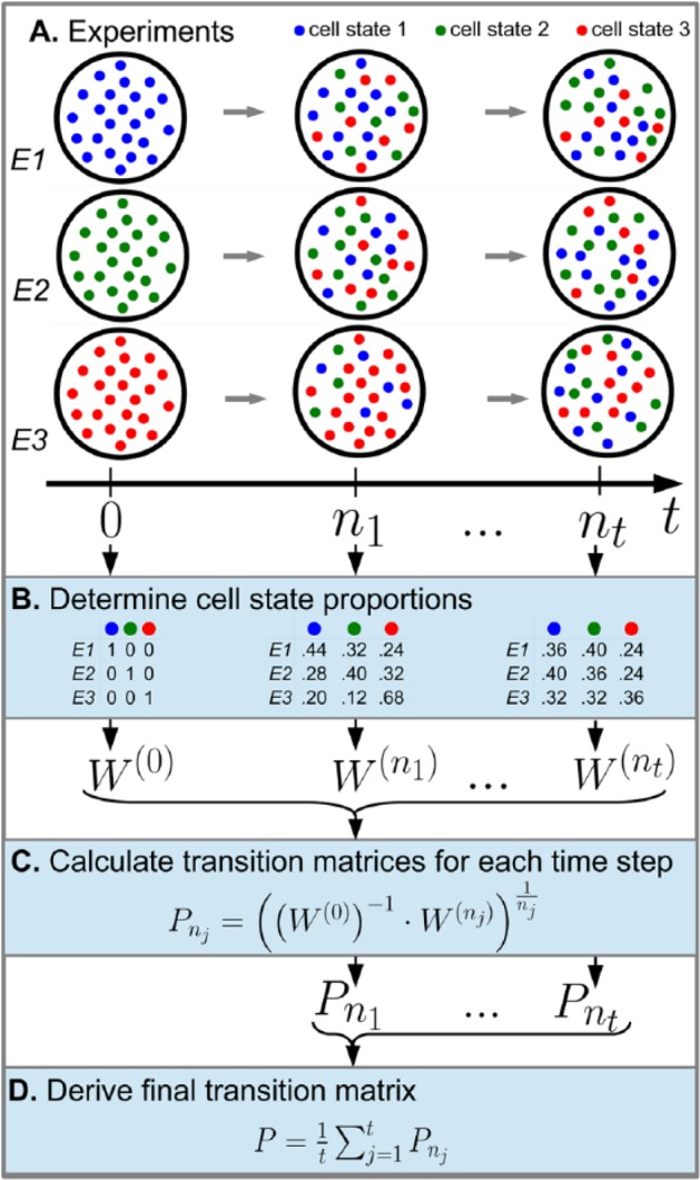
CellTrans application workflow. To demonstrate the general workflow of CellTrans, we use a fictive experiment with 3 illustrative cell states: 1 (blue), 2 (green), and 3 (red). (A) Three different fluorescence-activated cell sorting experiments E1, E2, and E3 with pure initial cell states and fictional evolutions of these proportions are illustrated. (B) The measured cell state compositions at times n_j are used to construct the cell state proportion matrix $W^{(n_j)}$, j = 1,…,t Here, each row corresponds to the cell state proportions of one experiment. (C) CellTrans estimates a transition matrix $P_{n_j}$ based on the cell state proportion matrix $W^{(n_j)}$ for each time point of measurement j = 1,…,t. (D) Finally, averaging the estimated transition matrices $P_{n_j}$ leads to the final transition matrix P.

We assume that each cell transitions from state i to state j during a time step of length τ with probability p_ij, i, j = 1,2,…, m. Note that the choice of the time step length has no substantial influence on the predictions which we discuss later. Furthermore, it is assumed that the transition probabilities are constant over time and do only depend on the state of the cell.⁴ These considerations lead to a discrete-time Markov process with transition matrix P = (p_ij)_{i, j=1,…,m} for the random evolution of the state of individual cells. Our goal is to estimate P, i.e., all transition probabilities between the cell states, from the experimental data stored in the matrices $W^{(n\_1)},\dots ,W^{(n_t)}$. The interaction graph of the underlying Markov model together with the transition probabilities is illustrated in Figure 5A.

Figure 5.

Transitions in the model and regularization of the matrix root. (A) CellTrans estimates the transition matrix of the underlying discrete-time Markov model. This matrix contains the transition probabilities between all cell states. Here, these transitions are illustrated for 3 fictive cell states. (B) to (D) We simulated cell state proportion data for an experiment with 3 fictive cell states in which regularization of the matrix roots is necessary to obtain a stochastic matrix. The dots represent simulated data points, and the solid curves represent the prediction of CellTrans. For details on the required matrix root regularization, see the main text.

Construction of data matrices

Let $w_k^{(0)}=\left\{w_{k1}^{(0)},\dots ,w_{km}^{(0)}\right\}$ denote the initial cell state proportions in the kth experiment which is a row vector of length m with non-negative entries summing to one. As explained before, m of those initial cell state proportions $w_1^{(0)},w_2^{(0)},\dots ,w_m^{(0)}$ are needed. The initial experimental matrix W⁽⁰⁾ is row-wise constructed from these cell state proportions, i.e.,

$$W^{(0)}=\left(\begin{array}{ccc}-& w_1^{(0)}& -\\ -& ⋮& -\\ -& w_m^{(0)}& -\end{array}\right)=\left(\begin{array}{ccc}{w}_{11}^{(0)}& \cdots & w_{1m}^{(0)}\\ ⋮& \ddots & ⋮\\ w_{m1}^{(0)}& \cdots & w_{mm}^{(0)}\end{array}\right)$$

An analytical requirement for the applicability of CellTrans is the existence of the inverse of W⁽⁰⁾. This can be assured by appropriate initial cell state proportions, e.g. by choosing purified initial cell cultures. Because this experimental setup is very common in FACS and flow cytometry experiments, it is implemented as default option in CellTrans. However, also an individually designed initial experimental matrix can be used.

In the experiments, the cell state proportions at each time point n₁, n₂,…, n_t have to be assessed. Let $w_k^{(n_j)}$ denote the cell state proportions of experiment k = 1,2,…, m after time n_j with j = 1,2,…, t. For each of these time points, a cell state proportion matrix after time n_j is obtained by constructing the matrix as described above for W⁽⁰⁾:

$$W^{(n_j)}=\left(\begin{array}{ccc}-& w_1^{(n_j)}& -\\ -& w_2^{(n_j)}& -\\ -& ⋮& -\\ -& w_m^{(n_j)}& -\end{array}\right)$$

Because each row describes the cell state proportions in the corresponding experiment, all rows sum up to one with non-negative entries. In total, t of such matrices need to be constructed from the experiments, one for each time point of measurement.

Derivation of transition matrices $P_{n_j}$

For each time point n_j with j = 1,2,…,t, CellTrans derives a transition matrix $P_{n_j}$ as follows. This derivation is based on the theory of Markov models.⁸ We use that the distribution of a Markov chain after n_j time steps can be obtained by multiplying the initial distribution with the transition matrix raised to the power of n_j; hence,

$$W^{(0)}{P}^{n_j}=W^{(n_j)}$$

Here, W⁽⁰⁾ denotes the initial experimental matrix and $W^{(n_j)}$ the cell state proportion matrix after time n_j. Because we are interested in the underlying transition matrix P, we solve this equation for P by multiplying with the inverse of W⁽⁰⁾ and computing the n_j th matrix root, i.e.,

$$P^{n_j}={\left(W^{(0)}\right)}^{-1}.W^{(n_j)}\text{and}{P}_{n_j}={\left({\left(W^{(0)}\right)}^{-1}.W^{(n_j)}\right)}^{\frac{1}{n_j}}$$ (1)

for j = 1,2,…,t. Here, we compute the so-called principal matrix root because matrix roots are not necessarily unique. For an overview of the existence and computation of matrix roots see the work by Higham and Lin.¹³ Note that the existence of (W⁽⁰⁾)⁻¹ is assured by the appropriate choice of the initial cell state proportions described earlier. The matrix $P_{n_j}$ is the estimated transition matrix derived from time point n_j. Although this derivation looks straightforward, there are potential analytical problems which are described in the following section.

Regularizing matrix roots to stochastic matrix roots

Importantly, equation (1) should yield a transition matrix of a Markov chain, i.e., a stochastic matrix with non-negative entries and row sums equal to one. However, the root of a stochastic matrix is not necessarily stochastic again.¹³ CellTrans verifies whether the matrix roots are stochastic or not. If not, the matrix roots are regularized to be stochastic with the quasi-optimization of the root matrix (QOM) algorithm which is sketched in the following section and described in detail in Kreinin and Sidelnikova.¹⁴

The QOM algorithm performs a row-wise Euclidean distance minimization by transforming each row of the matrix into a valid row of a transition matrix, i.e., a vector containing non-negative entries which sum to one. The result is a uniquely determined stochastic matrix which closely approximates the original matrix. In the work by Kreinin and Sidelnikova,¹⁴ the effect of QOM regularization on nonstochastic matrix roots is numerically investigated. The authors calculated the infinity matrix norm and also the mean absolute deviation of the difference between the QOM result and the original transition matrix for 32 examples of matrix regulation. This numerical comparison demonstrates a low approximation error of the QOM regularization.

Computation of the transition matrix P

CellTrans estimates the transition matrix P by averaging the transition matrices $P_{n_j}$ for each time point j = 1,2,…,t, i.e.,

$$P=\frac{1}{t}{\displaystyle \sum _{j=1}^t{P}_{n_j}}$$ (2)

This transition matrix is the final estimation of CellTrans quantifying the transition probabilities between all cell states. The overall workflow of CellTrans is summarized in Figure 1.

Note that the dynamics of the Markov chain model can also be described by a master equation, i.e., a set of first-order differential equations. The master equation reads

$$\frac{d}{dt}{a}_i(t)={\displaystyle \sum _{j\ne i}\left(p_{ji}{a}_j(t)-p_{ij}{a}_i(t)\right)i=1,\dots ,m}$$ (3)

with initial conditions a_i(0) = c_i.¹⁵ Here, a_i(t) describes the proportion of cells in state i at time t, and P = (p_ij)_{i, j =1,…,m} represents the estimated transition matrix from CellTrans. Hence, these differential equations describe the temporal evolution of the cell state proportions. We will use this master equation later to compare the results of CellTrans to those of ODE models.

Important functions in CellTrans

Here, we introduce the most important functions which are implemented in CellTrans. In the following sections, we will demonstrate the usage of these functions in several case studies.

readExperimentalData()

This function reads all necessary data. First, it opens a dialog box which asks for the number of cell types, the names of the cell types, the time step length τ, and the time points of measurement. Then, the files containing the cell state proportion matrices are read. First, the initial experimental setup matrix W⁽⁰⁾ can be chosen as identity matrix (for pure initial cell populations) or an individual initial matrix can be used. Then, the experimental cell proportion matrices are read for each time point of measurement. It is recommendable to save the input into a variable for further analysis, e.g. input <-readExperimentalData().

celltransitions(input)

This function derives and prints the estimated transition probabilities and the predicted equilibrium distribution. The variable input contains the read data from the function readExperimentalData().

celltrans_plot(input), celltrans_plotPDF(input)

These functions allow to create plots of the predictions of CellTrans and the experimental data. The variable input contains the read data from readExperimentalData().

timeToEquilibrium(input,initialDistribution,tol)

This function estimates the time from any initial cell state proportions until the equilibrium proportions are reached. The variable input contains the read data from the function readExperimentalData(). The variable initialDistribution is a vector of length m which describes the initial cell state proportions, e.g. c(0.25,0.25,0.25,0.25) for equal proportions of m = 4 cell types. The third parameter tol gives a tolerance deviation between the cell state proportions of the equilibrium distribution and those of the predicted cell state proportions, as the exact equilibrium distribution is not reached, in general. For the parameter tol, we recommend values between 0.01 and 0.02.

For a comprehensive introduction demonstrating the application of these functions, see the detailed vignette provided with the R package (Additional file 1—supplementary material).

Applications of CellTrans

CellTrans can be applied to analyze cell state proportion data from FACS and flow cytometry experiments with respect to several questions. The applications are based on the estimation of the transition probabilities of the underlying model as described above:

1. The estimated probabilities quantify the frequencies of state transitions and can be used to detect frequent, rare, or almost never occurring transitions. Such a prediction allows to hypothesize about biological mechanisms which are responsible for the observed transition structure, e.g. an underlying transition hierarchy.

2. Another application is the prediction of cell line compositions at any time point. Such an estimate can be used to predict cell line compositions even beyond the time periods of experiments which we will demonstrate in the “Results” section.

3. CellTrans can be used to estimate the equilibrium cell state proportions. This information can support experimentalists to decide whether experimentally observed cell line compositions already reached equilibrium.

4. CellTrans allows the prediction of the time needed to reach equilibrium proportions from any initial cell state composition. The choice of the time period of FACS experiments and the time points at which cell state compositions are measured is often difficult. Here, the estimate of the time needed to reach equilibrium can be useful.

Table 1 summarizes the main applications and the corresponding functions in CellTrans.

Table 1.

Main applications of CellTrans and corresponding implemented functions.

ESTIMATION OF	APPLICATION/INTERPRETATION	CORRESPONDING FUNCTION(S)
Transition probabilities	Quantification of cell state transitions Transition hierarchies Detect rare and frequent transitions and conclude responsible mechanisms	celltransitions()
Cell state compositions	Predictions beyond time period of experiments Validate experimental results	celltrans_plot() celltrans_plotPDF()
Equilibrium compositions	Predict equilibrium compositions Validate experimental results	celltransitions()
Time to equilibrium	Plan time periods of experiments Choice of time points of measurement	timeToEquilibrium()

Results

In this section, we apply CellTrans to publicly available data on the evolution of cell state proportions obtained from FACS and flow cytometry experiments. We point out possible conclusions that can be drawn from the application of CellTrans. The used data are provided in Additional file 2 (supplementary material) so that the results of this section can be reproduced.

Dynamics between cancer cell subpopulations in colon cancer

Background

There is evidence that CD133⁺ cells represent a cancer stem cell (CSC) subpopulation within SW620 human colon cells.⁶ In the work by Yang et al,⁶ the dynamics between CSCs and nonstem cancer cells (NSCCs) has been experimentally investigated. In detail, purified NSCCs and CSCs sorted from the SW620 cell line by FACS were cultured for 26 days, and the composition of these cultures was measured every second day in both experiments. Here, we analyze the data from these experiments with CellTrans and compare the resulting predictions with those obtained from an ODE model which has been analyzed in the work by Wang et al.⁵

Application of CellTrans

The experimental setup in the work by Yang et al ⁶ can be formulated within the framework of CellTrans as follows. There are m = 2 subpopulations considered in SW620 human colon cancer cells which are called CSC and NSCC. Note that the assumption that both of these cell types do not differ in their proliferation and death rates is justified.⁵ The initial experimental matrix representing purified initial cell cultures is as follows:

$$W^{(0)}=\left(\begin{array}{cc}1& 0\\ 0& 1\end{array}\right)$$

where the first row corresponds to the experiment with sorted CSCs and the second row with sorted NSCCs. Hence, we choose the identity matrix in CellTrans as initial experimental matrix.

There are in total 12 time points of cell state proportion measurements which are given by 2, 4, 6, 8, 10, 12, 14, 16, 18, 20, 22, and 24 days. Thus, it is sensible to choose a time step length τ of 1 day. The cell state proportion matrices for each of these time points can be derived from the experimental data provided in Tables S2 and S3 in the work by Wang et al⁵ which leads to 12 corresponding cell state proportion matrices. These matrices are provided in .TXT files in Additional file 1 (supplementary material). For example, the cell state proportion matrix after 8 days is as follows:

$$W^{(8)}=\left(\begin{array}{cc}1.7150& 1.2850\\ 1.5523& 1.4477\end{array}\right)$$

That is, the experiment starting with 100% CSCs evolved to 71.5% CSCs and 28.5% NSCCs, and the experiment starting with pure NSCCs evolved to 55.23% CSCs and 44.77% NSCCs after 8 days, respectively.

The function CellTransitions(input) allows to derive the transition probabilities between the cell states and the predicted equilibrium distribution. CellTrans derives a transition matrix for each of the 12 cell state proportion matrices. Note that none of these matrices require regularization by the QOM algorithm because the matrix roots are already stochastic matrices. For example, the transition matrix derived from the experimental data after 8 days W⁽⁸⁾ is as follows:

$$P_8=\left(\begin{array}{cc}1.9309& 1.0691\\ 1.1339& 1.8661\end{array}\right)$$

Finally, the transition matrix P is obtained by computing the average of the 12 transition matrices from each time point, i.e.,

$$P=\frac{1}{12}{\displaystyle \sum _{j=1}^{12}{P}_{n_j}}=\left(\begin{array}{cc}1.9455& 1.0545\\ 1.1030& 1.8970\end{array}\right)$$

which is an estimate of the transition probabilities between NSCC and CSC per day. For example, a CSC converts with probability 0.0545 to an NSCC or an NSCC converts with probability 0.1030 to a CSC within a day. The predicted long-term cell state proportions can be obtained by CellTrans from the steady state of the transition matrix P and are also provided by the function CellTransitions(input) which yields the following:

$$w*=\left(\begin{array}{c}1.654\\ 1.346\end{array}\right)$$

That is, CellTrans predicts a proportion of 65.4% CSCs and of 34.6% NSCCs after sufficient time. The time from 100% CSCs to the equilibrium composition can be estimated with the command timetoEquilibrium(input,c(1,0),0.01) which yields 21 days. Similarly, the time from 100% NSCCs to the equilibrium composition can be estimated with the command timetoEquilibrium(input,c(0,1),0.01) which yields 25 days. Therefore, the time of the experiment was sufficient to reach the equilibrium in this case.

Model comparison

In the work by Wang et al,⁵ the dynamics between CSCs and NSCCs has been modeled by an ODE model with 8 parameters. Some of these parameters have been collected from in situ experiments (see Table 1). The predictions from our model show a much better accordance to the data than the predictions of the ODE model (root mean square deviation (RMSD) CellTrans vs ODE: 0.03737 vs 0.09874 for the experiment starting with pure CSC cultures, RMSD CellTrans vs ODE: 0.05326 vs 0.10484 for the experiment starting with pure NSCC cultures). A comparison between the original data from the work by Wang et al⁵ and the predictions of the derived Markov chain is shown in Figure 2A illustrating that the estimated Markov model well describes the experimental data.

Figure 2.

Comparison of model predictions for colon cancer cell lines. (A) We used CellTrans to analyze data about the evolution of cancer cell line compositions from Yang et al.⁶ The involved cell states are cancer stem cells (CSCs) and nonstem cancer cells (NSCCs), and the original data are plotted as colored dots including the experimental standard deviation. The red curve is the prediction of the cell state compositions of the experiment starting with pure CSCs and the blue curve represents the prediction starting with pure NSCCs. The gray line corresponds to the predictions of ordinary differential equation (ODE) models which have been proposed in the original study.⁶ (B) Analysis of colon cancer cell line data from Geng et al⁷ with the cell states adherent and suspended. The red curve is the prediction of CellTrans for the experiment starting with adherent cells only, and the blue curve is the corresponding prediction starting with suspended cells. The gray line is the prediction of the ODE model introduced in the work by Geng et al.⁷

We can use the master equation (3) to equivalently describe the cell state dynamics with an ODE system

$$\begin{array}{l}\frac{d}{dt}CSC(t)=-1.0545CSC(t)+1.103NSCC(t)\\ \frac{d}{dt}NSCC(t)=1.0545CSC(t)-1.1030NSCC(t)\end{array}$$

with appropriate initial conditions CSC(0) = 1, NSCC(0) = 0 for the experiment with pure CSCs in the beginning. The solution

$$\begin{array}{l}CSC(t)=1.346e^{-1.1575t}+1.654\\ NSCC(t)=-1.346e^{-1.1575t}+1.346\end{array}$$

allows to obtain the steady state by letting t → ∞

Summary

This case study demonstrates that the Markov model underlying CellTrans is potentially able to make better predictions than more complex ODE models with parameter calibration. The experimental data on the evolution of cell state proportions are sufficient to interpolate the data. Moreover, the equilibrium proportion is reliably predicted.

Dynamic switch between adhesive and suspended cell types in colon cancer

Background

In the work by Geng et al,⁷ the dynamic switch between 2 different adhesion phenotypes in colorectal cancer cells has been analyzed. The involved cell states in this study are adherent and suspended cells. Both of these cell types have been separated and replated. Subsequently, both initially pure cell cultures have been monitored for 8 hours, and the cell state proportions have been measured after 0.5 and 1 hours and subsequently in 2-hour intervals.

Application of CellTrans

The study can be integrated in the CellTrans framework in the following way. There are m = 2 cell states: adherent and suspended. Although there is no explicit statement regarding the proliferation rates in the work by Geng et al,⁷ we assume equal rates because the authors model the evolution of the cell state proportions without considering effects of proliferation. The initial experimental matrix is given by the identity matrix because the experimental initial cell state proportions are pure cell cultures of both phenotypes. Here, the first row corresponds to the experiment with 100% adherent cells and the second row with 100% suspended cells.

Subsequently, the cell state proportion matrices for t = 6 time points (at 0.5, 1, 2, 4, 6, and 8 hours) can be deduced from the experiments. Here, the time step length τ is chosen to be 1 hour. The matrices are provided in Additional file 1 (supplementary material).

Subsequently, CellTrans derives transition matrices for each of these cell state proportion matrices. This leads to 6 transition matrices P_0.5, P₁, P₂, P₄, P₆, and P₈. All of these matrices do not require regularization in this case because all of them are already stochastic matrices.

Finally, the transition matrix P is obtained as average:

$$P=\frac{P_{1.5}+P_1+P_2+P_4+P_6+P_8}{6}=\left(\begin{array}{cc}1.8612& 1.1388\\ 1.2908& 1.7092\end{array}\right)$$

The predicted cell state proportions based on the estimated transition matrix and the experimental data are plotted in Figure 2B.

The steady state of the derived transition matrix P is given as follows:

$$w*=\left(\begin{array}{c}1.6768\\ 1.3232\end{array}\right)$$

That is, the long-term cell state proportions of adherent and suspended cells are predicted as 67.68% and 32.32%, respectively. This prediction is in good accordance with the corresponding experimentally observed equilibrium proportions described in the work by Geng et al.⁷

Model comparison

Geng et al⁷ formulated a mathematical ODE model to describe the dynamics for the adherent and the suspended cells to reestablish the equilibrium ratio. Note that this approach requires to fit the analytical solution of the model to the experimental data. The fit in the work by Geng et al⁷ yields the solution adh(t) = 0.3e^−0.5t +0.7.

In contrast, we can derive an alternative ODE system with the same structure using the master equation (3) based on the predictions of CellTrans, i.e.,

$$\begin{array}{l}\frac{d}{dt}adh(t)=-1.1388adh(t)+1.2908susp(t)\\ \frac{d}{dt}susp(t)=1.1388adh(t)-1.2908susp(t)\end{array}$$

with initial conditions adh(0) = 1, susp(0) = 0. The solution

$$\begin{array}{l}adh(t)=1.323e^{-1.4296t}+1.67\\ susp(t)=-1.323e^{-1.4296t}+1.323\end{array}$$

is close to the solution in the work by Geng et al⁷ and allows to predict the equilibrium distribution by letting t → ∞. This equilibrium solution well corresponds to the experimental findings.

The predictions of CellTrans and the ad hoc ODE in the work by Geng et al⁷ are in good accordance with the original data (RMSD CellTrans vs ODE: 0.0219 vs 0.0278 for the experiment starting with pure adherent cultures and RMSD CellTrans vs ODE: 0.02709 vs. 0.02407 for the experiment starting with pure suspended cultures) (see also Figure 2B).

Summary

It remains unclear in which way the “best-fit” solution in the introduced ODE approach in the work by Geng et al⁷ has been obtained. Instead of fitting parameters, our approach offers a transparent estimation of the underlying transition matrix yielding good predictions. Moreover, especially from the point of view of an experimentalist, the automated estimation by CellTrans does not require a deeper engagement with mathematical modeling.

Proportions of stem-like, basal, and luminal phenotypes in breast cancer

Background

The dynamics of phenotypic proportions in human breast cancer cell lines is studied by Gupta et al.⁴ In detail, the authors used FACS analysis to isolate three mammary epithelial cell states (stem-like, basal, and luminal) from the SUM159 and SUM149 breast cancer cell lines. Pure subpopulations of the three cell states have been cultured for 6 days, and cell state proportions have been measured at the end of the experiment.

Application of CellTrans

We apply CellTrans to both cell lines, SUM149 and SUM159. The proliferation rates of the involved cell types are equal.⁴ The initial experimental cell proportions in both cases can be described as follows:

$$W^{(0)}\left(\begin{array}{ccc}1& 0& 0\\ 0& 1& 0\\ 0& 0& 1\end{array}\right)$$

where the first line corresponds to the experiment with sorted stem-like cells, the second row to sorted basal cells, and the third row to sorted luminal cells.

The proportions of cell states have been obtained at a single time point after 6 days. The time step length τ is 1 day in this case. For SUM149, the following cell state proportion matrix can be obtained from the work by Gupta et al⁴:

$$W^{(6)}=\left(\begin{array}{ccc}0.053& 0.168& 0.78\\ 0.026& 0.504& 0.47\\ 0.013& 0.007& 0.98\end{array}\right)$$

where the first row contains the cell state proportions of the experiment with sorted stem-like cells, the second row with sorted basal cells, and the third row with sorted luminal cells in the beginning, respectively.

Using the function celltransitions(input), CellTrans derives the following transition matrix from this time point:

$$P_6=\left(\begin{array}{ccc}0.5814& 0.1102& 0.3084\\ 0.0145& 0.8887& 0.0968\\ 0.0058& 0.0006& 0.9936\end{array}\right)$$

which yields the final transition probabilities because there is only one time point of measurement in this case. For example, the second row indicates that basal cells transition to stem-like cells within a day with a probability of 1.45%, do not change their state with a probability of 88.87%, and convert to the luminal state with a probability of 9.68%. A similar derivation leads to the transition probabilities for SUM159 which exhibits different transition dynamics.

The predicted equilibrium distribution of our model for SUM149 is

$$w^{*}=\left(1.0141.0191.967\right)$$

and for the SUM159 cell line

$$w^{*}=\left(1.02351.97341.0031\right)$$

(first entry stem-like, second basal, and third luminal) (see Figure 3A to F). These plots can be created in CellTrans with the command celltrans_plot(input). The predictions are in good accordance with the original tumor compositions. In detail, the SUM149 tumor sample is composed of 3.9% stem, 3.3% basal, and 92.8% luminal cells. The proportions within the SUM159 cell line is 1.9% stem, 97.3% basal, and 0.62% luminal cells.⁴

Figure 3.

CellTrans model predictions and validations. (A) to (G) We used CellTrans to analyze data of the evolution of cell state proportions of publicly available data. The data are plotted by colored dots. (A) to (F) The data originate from the work by Gupta et al4 with 3 different cell states (stem, basal, and luminal) from SUM149 and SUM159 breast cancer cell lines. The predictions of our analysis are plotted by colored curves. The color indicates the state of the cells at the beginning of the corresponding experiment. (G) Analysis of composition data (dots) of human mammary epithelial cell lines¹⁶ with cell states CD44−/CD24+ and CD44+/CD24−. The corresponding predictions are plotted as colored curves. (H) to (I) We excluded several of the late data points from the data of the proportions of cancer stem cells (CSCs) and nonstem cancer cells from the work by Yang et al⁶ and the data with adherent and suspended cells from the work by Geng et al.⁷ The predictions based on the remaining data are plotted, compare also with Figure 2. This investigation indicates that CellTrans is able to predict cell state proportions even beyond the duration of experiments and that only a few data points are needed to reliably predict the equilibrium.

The time from 100% stem-like cells to the predicted equilibrium composition can be estimated by CellTrans with the command timetoEquilibrium(input,c(1,0,0),0.01) which yields 31 days. In contrast, the command timeToEquilibrium(input,c(0,0,1),0.01) gives an estimation of 8 days to reach the equilibrium from 100% luminal cells. These predictions reflect that purified luminal cells are much closer to the equilibrium composition than purified stem-like cells.

Comparison with previously used Markov model

Gupta et al⁴ introduced a Markov model of cell state transitions to explain the observed equilibrium. The predictions are based on a single time point, and no regularization of the matrix root is required. CellTrans is able to recover the transition matrices for both cell lines SUM149 and SUM159 presented in the work by Gupta et al⁴ (Table 1). Figure 3A to F illustrates the predicted evolution of cell fractions for both cell lines.

The master equation (3) can also be applied to derive an equivalent ODE system:

$$\begin{array}{l}\frac{d}{dt}stem\left(t\right)=-1.4186stem\left(t\right)+1.0145bas\left(t\right)+1.0058lum\left(t\right)\\ \frac{d}{dt}bas\left(t\right)=1.1102stem\left(t\right)-1.1113bas\left(t\right)+1.0006lum\left(t\right)\\ \frac{d}{dt}lum\left(t\right)=1.3084stem\left(t\right)+1.0968bas\left(t\right)-1.0064lum\left(t\right)\end{array}$$

The solution for the initial conditions stem(0) = 1, bas(0) = 0, lum(0) = 0 reads

$$\begin{array}{l}stem\left(t\right)=1.0141+1.9771e^{-1.4274t}+1.0088e^{-1.1089t}\\ bas\left(t\right)=1.0191-1.3394e^{-1.4274t}+1.3203e^{-1.1089t}\\ lum\left(t\right)=1.9668-1.6377e^{-1.4274t}-1.3291e^{-1.1089t}\end{array}$$

Summary

Several applications of our model are demonstrated here. First, CellTrans is able to analyze arbitrarily many cell states, not only 2. Second, the original tumor composition, which is not included in the analysis, is precisely predicted. Third, the estimation of the time to the equilibrium composition potentially helps experimentalists in planning the time periods of cell line experiments.

Epithelial-mesenchymal transition in breast cancer

Background

To investigate the epithelial-mesenchymal transition (EMT) and its implication on the development and progression of breast cancer, Mani et al¹⁶ induced an EMT in nontumorigenic, immortalized human mammary epithelial cells (HMLEs). Subsequently, they used flow cytometry analysis to sort the cells based on the expression of CD44 and CD24, 2 cell surface markers whose expression in the CD44⁺/CD24⁻ configuration is associated with both human breast CSCs and normal mammary epithelial stem cells. One of their aims was to determine whether the CD44⁺/CD24⁻ cells isolated from monolayer cultures of HMLE cells could generate CD44⁻/CD24⁺ cells in vitro.

To examine this question, the authors cultured purified cell phenotypes into monolayer cultures and assayed for the appearance of other cell phenotypes during time. The results of these experiments are summarized in Table S1.¹⁶

Application of CellTrans

This experimental setup can be formulated within the CellTrans framework as follows. There are m = 2 cell states which are named CD44⁺/CD24⁻ and CD44⁻/CD24⁺. The initial experimental matrix is given by the identity matrix. This matrix is constructed such that the first row represents the pure CD44⁺/CD24⁻ initial cell culture, and the second row corresponds to pure CD44⁻/CD24⁺ cell culture.

The cell state proportions have been experimentally determined for t = 4 time points (at 2, 4, 6, and 8 days). Here, the time step length τ is 1 day. The cell state proportions matrices W⁽²⁾, W⁽⁴⁾, W⁽⁶⁾, and W⁽⁸⁾ can be constructed from the data in Mani et al,¹⁶ e.g.

$$W^{(4)}=\left(\begin{array}{cc}1.70& 1.30\\ 1.01& 1.99\end{array}\right)$$

where the first row represents the experiments starting with pure cultures of cell phenotype CD44⁺/CD24⁻ and the second row with cell phenotype CD44⁻/CD24⁺, respectively. The files containing these matrices are provided in Additional file 1 (supplementary material).

CellTrans estimates transition matrices for each of the cell state proportion matrices. This approach leads to 4 matrices P₂, P₄, P₆, and P₈. In this case, all of the derived matrices do not require regularization because all matrices are already stochastic matrices. The transition matrix P is obtained by averaging over the derived transition matrices which yields the following:

$$P=\frac{P_2+P_4+P_6+P_8}{4}=\left(\begin{array}{cc}1.8868& 1.1132\\ 1.0007& 1.9993\end{array}\right)$$

The predicted cell state proportions of this transition matrix with the initial states from the experiments and the experimental data are plotted in Figure 3G.

The solution of the master equation (3) for the experiment with pure CD44⁺/CD24⁻ cells in the beginning is as follows:

$$\begin{array}{l}CD{44}^{+}/CD{24}^{-}(t)=1.0006e^{-1.1133t}+1.9994\\ CD{44}^{-}/CD{24}^{+}(t)=-1.0006e^{-1.1133t}+1.0006\end{array}$$

Summary

This case study demonstrates two potential applications of CellTrans. First, CellTrans can reveal rare cell transitions which are indicated by the estimated probability to convert from CD44⁻/CD24⁺ to CD44⁺/CD24⁻ of 0.0007 per day. Hence, transitions from CD44⁻/CD24⁺ to CD44⁺/CD24⁻ cells almost never occur suggesting a potential cell transition hierarchy.

Second, the experiments only cover the first 8 days after culturing, but the time period until the equilibrium proportions are reached is not clear from the beginning. Here, the predicted equilibrium distribution is given as follows:

$$w^{*}=\left(\begin{array}{c}1.0063\\ 1.9937\end{array}\right)$$

which corresponds to an equilibrium proportion of 0.63% of CD44⁺/CD24⁻ and 99.37% of CD44⁻/CD24⁺. CellTrans can estimate the expected time until this equilibrium is reached. The command timetoEquilibrium(input,c(1,0),0.01) estimates the expected time to the equilibrium starting with a pure CD44⁺/CD24⁻ cell line composition with a tolerance deviation of 1%. With these parameters, CellTrans predicts a time of 39 days until the equilibrium proportions are reached.

Influence of the choice of the time step length τ

To demonstrate that the predictions and results of CellTrans are independent of the choice of the time step length τ, we varied τ in the case studies with data from the works by Wang et al⁵ and Geng et al.⁷ We predicted the equilibrium distribution, the expected time to equilibrium, and the predicted cell state composition after an arbitrary time for different time step lengths. The results are summarized in Additional file 3 (supplementary material) and indicate that the predictions are not influenced by τ.

Validation of the predicted equilibrium of CellTrans

One important application of CellTrans is the prediction of the equilibrium of cell state proportions and the time needed to reach this equilibrium. In some experiments, the equilibrium proportions are not reached at the end of the experiment, e.g. in the investigation of the EMT in breast cancer introduced above.¹⁶ Here, we show that CellTrans is able to make predictions beyond the duration of the experiments. In detail, CellTrans is able to reliably predict both the equilibrium cell state proportions and the time needed to reach this proportion. To demonstrate this, we performed a validation analysis based on the 2 case studies dealing with colon cancer cells.^6,7 We used only a subset of the available data points to create predictions of the cell state proportions over time with CellTrans. We excluded late data points to mimic an experimental situation in which the equilibrium is not reached yet. The results of this validation study are illustrated in Figure 3H to I. It turns out that only a few data points are sufficient to reliably predict the equilibrium cell state proportions. Moreover, the predicted time to reach equilibrium proportions is very robust with respect to the choice of available data points. This investigation indicates that CellTrans is able to make predictions even beyond the time period of experiments and might therefore also support the planning of experimental time periods.

Influence of nonpure initial cell state compositions

As our case studies demonstrate, most FACS and flow cytometry experiments are based on pure initial cell state compositions. However, CellTrans can also be used to analyze experimental data with nonpure initial compositions. Here, we demonstrate this possibility and investigate whether the predictions and results are influenced by such an initial composition. For this, we reused data from the works by Yang et al⁶ and Geng et al⁷ but excluded several of the first data points such that the initial cell state compositions are nonpure. We then used CellTrans to estimate a transition matrix based on these remaining data and compare the corresponding predictions with the original estimates derived from all available data. It turns out that both the evolution of cell line compositions and the equilibria are reliably predicted with nonpure initial cell state compositions. The results of this analysis are illustrated in Figure 4.

Figure 4.

Influence of nonpure initial cell state compositions. To obtain nonpure initial cell state proportions, we excluded several of the early data points, as indicated in the legends, from the case studies with data from the works by Yang et al⁶ and Geng et al.⁷ The plotted predictions in both figures are based on the analysis of the remaining data points with CellTrans. The starting point of each curve indicates the initial cell state composition. Data from the works by (A) Yang et al⁶ and (B) Geng et al.⁷ CSC indicates cancer stem cell.

A simulation study demonstrating matrix regularization

The presented case studies so far do not require matrix regularization; ie, the matrix roots that CellTrans calculate are already stochastic matrices. To demonstrate that such a regularization might be necessary, we introduce a simulation study and explain how the QOM algorithm performs the necessary regularization.

In the simulation study, we assume the existence of m = 3 cell states. We simulate 3 experiments starting with pure cultures of each cell state. Hence, the experimental initial matrix is as follows:

$$W^{(0)}=\left(\begin{array}{ccc}1& 0& 0\\ 0& 1& 0\\ 0& 0& 1\end{array}\right)$$

As time points, we choose t = 2τ, 4τ, 6τ. Here, τ is an arbitrary time step length.

We created an arbitrary transition matrix to describe the transition probabilities between the 3 cell states:

$$P_{sim}=\left(\begin{array}{ccc}1.7739& 1.1762& 1.0499\\ 1.0006& 1.8210& 1.1784\\ 1.0937& 1.0712& 1.8351\end{array}\right)$$

The Markov chain associated with this transition matrix has the steady-state distribution:

$$w_{sim}^{*}=\left(1.18721.36321.4496\right)$$

Then, we generated experimental data after times 2τ, 4τ, and 6τ from the matrix powers P², P⁴, and P⁶. We also added a normally distributed noise with mean 0 and a standard deviation of 0.01 to reflect unprecise measurements. This led to the following cell state proportion matrices:

$$\begin{array}{l}{W}^{(2)}=\left(\begin{array}{ccc}0.6028& 0.2769& 0.1203\\ 0.0087& 0.7003& 0.2910\\ 0.1526& 0.1224& 0.7250\end{array}\right),\\ W^{(4)}=\left(\begin{array}{ccc}0.3934& 0.3819& 0.2247\\ 0.0492& 0.5175& 0.4333\\ 0.1989& 0.2465& 0.5546\end{array}\right),\\ W^{(6)}=\left(\begin{array}{ccc}0.2824& 0.4050& 0.3126\\ 0.1044& 0.4489& 0.4467\\ 0.2191& 0.2862& 0.4947\end{array}\right)\end{array}$$

Applying formula (1) to derive the matrix roots does not yield a stochastic matrix for all of these 3 matrices. The fourth matrix root of W⁽⁴⁾ is as follows:

$$\left(\begin{array}{ccc}0.7822& 0.1737& 0.0441\\ -0.0102& 0.8205& 0.1896\\ 0.0943& 0.0792& 0.8265\end{array}\right)$$

which is not a stochastic matrix due to the negative entry in the second row. The QOM algorithm transforms this matrix root into the stochastic matrix:

$$P_4=\left(\begin{array}{ccc}0.7822& 0.1737& 0.0441\\ 0.0000& 0.8154& 0.1846\\ 0.0943& 0.0792& 0.8265\end{array}\right)$$

The further derivation is continued with this regularized matrix root.

Finally, CellTrans derives the transition matrix:

$$P=\left(\begin{array}{ccc}0.7786& 0.1708& 0.0506\\ 0.0000& 0.8258& 0.1742\\ 0.0951& 0.0694& 0.8355\end{array}\right)$$

which is close to the originally generated P_sim. Furthermore, the steady state of the process associated with P is as follows:

$$w^{*}=\left(1.1911.36441.4446\right)$$

The effect of the QOM regularization on the prediction of CellTrans in this case is visualized in Figure 5B to D.

Discussion

Characteristic equilibrium proportions of distinct cell states are commonly observed in vivo and in vitro. Normal and cancerous cell lines exhibit and are able to maintain such an equilibrium.^4,5,7,16 Understanding the mechanisms which are responsible for this observation is important to develop appropriate therapies against cancer. There is evidence that stochastic transitions between different cell states can lead to such an equilibrium. To infer the underlying transition dynamics and to quantify these transitions is a key to understand and control the origin of such an equilibrium.

We introduce CellTrans, an automated framework to deduce the transition probabilities between different cell states from FACS and flow cytometry experiments, in which no differences in the proliferative properties between cell states are observed. The key assumption of the underlying mathematical model is that cells stochastically transition between different states and that the rates for these transitions only depend on the current state of the cell.

We point out that the transition probabilities can be derived on the basis of Markov chain theory by determining matrix roots from appropriately arranged data matrices and regularizing them to stochastic matrices if necessary. We discuss which mathematical challenges can occur and demonstrate how these challenges are handled by CellTrans. We use the QOM algorithm ¹⁴ to achieve matrix regularization and provide a simulation study which demonstrates that regularization might be necessary and how it can be achieved by the QOM algorithm.

To ensure a reliable estimation of cell state transitions, the cell state proportion data should be obtained on the basis of a large number of cells. This ensures the validity of the estimation based on the law of large numbers.¹⁵ We suggest to use at least 100 cells in each cell culture experiment to obtain the data for CellTrans.

Our stochastic approach on the basis of a Markov model can be translated into a system of first-order ODEs with the help of the master equation (3). The predictions of these ODEs are equivalent to those of the underlying Markov model of CellTrans. We demonstrate that CellTrans is able to predict the evolution of cell state proportions even more precisely compared with more complicated ODE models which use in situ parameter estimation, as, e.g. in the work by Wang et al.⁵

The analyzed case studies in this work demonstrate that CellTrans can be used to compare different cell types with respect to their ability to convert to other cell types, their frequency within equilibrium proportions, and their position within an existing cell transition hierarchy. We showed that the main application of CellTrans is the quantitative inference of transitions between distinctive cell types. The resulting transition probabilities allow to estimate which transitions occur frequently, rarely, or even almost never. Therefore, CellTrans might be able to reveal a hierarchy with respect to the importance of specific transitions for maintaining the observed equilibrium distributions.

The steady state derived by CellTrans can be interpreted as prediction of the equilibrium cell state proportions. Moreover, CellTrans is able to predict the duration from any initial experimental setup to such an equilibrium (see Figure 3H to I).

As demonstrated in Figure 3A to F, even patients classified to have the same type of tumor exhibit different equilibrium distributions. Hence, the dynamics of the cell state transitions is patient specific. CellTrans is able to predict these patient-specific transitions and can therefore be used to reveal differences within the same tissue in different patients. These predictions might be a step toward individual therapies.

Although the presented case studies in this work deal with disease-related cell line experiments, CellTrans can also be used to analyze nondiseased cell lines, such as immunostained progenitor cells, as long as the underlying model prerequisites are fulfilled. Hence, CellTrans can be used to analyze all cell line experiments in which cell state transitions only depend on the current state of the cell, and cell proliferation and death rates are equal.

We focus here on the case in which cell states exhibit similar proliferation and death rates. In principle, it would be possible to apply a similar approach also if this prerequisite is not fulfilled. This would first require to formulate an extended and more complicated mathematical model which is a challenging task for future work.

Our case studies demonstrate that CellTrans is a valuable tool to model and quantify cell state transitions. Experimentalists only have to validate the model assumptions. Then, the whole process of mathematical modeling and estimation is automatized. CellTrans allows versatile experiments by being able to analyze also cell state data originating from nonpure initial cell state distributions. In summary, CellTrans is an automated tool that facilitates the analysis and interpretation of cell state proportion data from these experiments on the basis of a Markov model for cell state transitions.

Additional Files (supplementary material)

Additional file 1 (pdf)—Vignette: A quick guide to CellTrans. A comprehensive example demonstrating how CellTrans can be used.

Additional file 2 (zip)—Cell state proportion matrices of the case studies. Additional file containing text files with cell state proportion matrices of the introduced case studies. These data can directly be used for the analysis with CellTrans.

Additional file 3 (pdf)—The influence of the time step length. Predictions of CellTrans for varying time step lengths τ for case studies by Yang et al⁶ and Geng et al.⁷

REFERENCES

- 1.Biteau B, Hochmuth CE, Jasper H. Maintaining tissue homeostasis: dynamic control of somatic stem cell activity. Cell Stem Cell. 2011;9:402–411. doi: 10.1016/j.stem.2011.10.004. [DOI] [PMC free article] [PubMed] [Google Scholar]
- 2.Hanahan D, Weinberg RA. The hallmarks of cancer. Cell. 2000;100:57–70. doi: 10.1016/s0092-8674(00)81683-9. [DOI] [PubMed] [Google Scholar]
- 3.Lopez-Bertoni H, Li Y, Laterra J. Cancer stem cells: dynamic entities in an ever-evolving paradigm. Biol Med. 2015;2015 doi: 10.4172/0974-8369.1000S2-001. [DOI] [PMC free article] [PubMed] [Google Scholar]
- 4.Gupta PB, Fillmore C, Jiang G, et al. Stochastic state transitions give rise to phenotypic equilibrium in populations of cancer cells. Cell. 2011;146:633–644. doi: 10.1016/j.cell.2011.07.026. [DOI] [PubMed] [Google Scholar]
- 5.Wang W, Quan Y, Fu Q, et al. Dynamics between cancer cell subpopulations reveals a model coordinating with both hierarchical and stochastic concepts. PLoS ONE. 2014;9:e84654. doi: 10.1371/journal.pone.0084654. [DOI] [PMC free article] [PubMed] [Google Scholar]
- 6.Yang G, Quan Y, Wang W, et al. Dynamic equilibrium between cancer stem cells and non-stem cancer cells in human sw620 and mcf-7 cancer cell populations. Br J Cancer. 2012;106:1512–1519. doi: 10.1038/bjc.2012.126. [DOI] [PMC free article] [PubMed] [Google Scholar]
- 7.Geng Y, Chandrasekaran S, Agastin S, Li J, King MR. Dynamic switch between two adhesion phenotypes in colorectal cancer cells. Cell Mol Bioeng. 2014;7:35–44. doi: 10.1007/s12195-013-0313-8. [DOI] [PMC free article] [PubMed] [Google Scholar]
- 8.Brémaud P. Markov Chains: Gibbs Fields, Monte Carlo Simulation, and Queues. Vol. 31. Berlin, Germany: Springer; 2013. [Google Scholar]
- 9.Buder T, Deutsch A, Klink B, Voss-Böhme A. Model-based evaluation of spontaneous tumor regression in pilocytic astrocytoma. PLoS Comput Biol. 2015;11:e1004662. doi: 10.1371/journal.pcbi.1004662. [DOI] [PMC free article] [PubMed] [Google Scholar]
- 10.Foo J, Leder K, Michor F. Stochastic dynamics of cancer initiation. Phys Biol. 2011;8:015002. doi: 10.1088/1478-3975/8/1/015002. [DOI] [PMC free article] [PubMed] [Google Scholar]
- 11.Komarova L, Sengupta A, Nowak MA. Mutation-selection networks of cancer initiation: tumor suppressor genes and chromosomal instability. J Theor Biol. 2003;223:433–450. doi: 10.1016/s0022-5193(03)00120-6. [DOI] [PubMed] [Google Scholar]
- 12.Herzenberg LA, Parks D, Sahaf B, Perez O, Roederer M, Herzenberg LA. The history and future of the fluorescence activated cell sorter and flow cytometry: a view from Stanford. Clin Chem. 2002;48:1819–1827. [PubMed] [Google Scholar]
- 13.Higham NJ, Lin L. On p th roots of stochastic matrices. Lin Algebra Appl. 2011;435:448–463. [Google Scholar]
- 14.Kreinin A, Sidelnikova M. Regularization algorithms for transition matrices. Algo Res Quart. 2001;4:23–40. [Google Scholar]
- 15.Gardiner CW. Stochastic Methods. Vol. 4. Berlin, Germany: Springer-Verlag; 1985. [Google Scholar]
- 16.Mani SA, Guo W, Liao M-J, et al. The epithelial-mesenchymal transition generates cells with properties of stem cells. Cell. 2008;133:704–715. doi: 10.1016/j.cell.2008.03.027. [DOI] [PMC free article] [PubMed] [Google Scholar]
Associated Data
This section collects any data citations, data availability statements, or supplementary materials included in this article.
Supplementary Materials